Synchronization of rotating helices by hydrodynamic interactions

Abstract

Some types of bacteria use rotating helical flagella to swim. The motion of such organisms takes place in the regime of low Reynolds numbers where viscous effects dominate and where the dynamics is governed by hydrodynamic interactions. Typically, rotating flagella form bundles, which means that their rotation is synchronized. The aim of this study is to investigate whether hydrodynamic interactions can be at the origin of such a bundling and synchronization. We consider two stiff helices that are modelled by rigidly connected beads, neglecting any elastic deformations. They are driven by constant and equal torques, and they are fixed in space by anchoring their terminal beads in harmonic traps. We observe that, for finite trap strength, hydrodynamic interactions do indeed synchronize the helix rotations. The speed of phase synchronization decreases with increasing trap stiffness. In the limit of infinite trap stiffness, the speed is zero and the helices do not synchronize.

1 Introduction

Many types of bacteria, such as certain strains of Escherichia coli or Salmonella typhimurium, swim by rotating flagellar filaments, which are several micrometers long and about 20 nm in diameter (the size of the cell body is about 1 $\mu$m) ber73 ; mac87 ; tur00 ; ber03 ; ber04 . The complete flagellum consists of three parts: the basal body which is a reversible rotary motor embedded in the cell wall, the helical filament that acts as propellor, and in-between a short flexible coupling called the proximal hook mac87 ; tur00 ; ber03 ; ber04 . The motor is powered by protons moving down an electrochemical gradient mac87 ; ber03 ; ber04 , which generates a constant torque independent of the dynamic load ber03 ; man80 . The rotation rates for the flagella of freely moving bacteria are of the order of 100 Hz tur00 ; ber03 ; ber04 . The filaments are polymers with high flexural and torsional stiffness mac87 ; ber03 ; ber04 . However, they are flexible enough to switch between different helical forms with distinct curvature and twist tur00 ; ber03 ; ber04 .

Typically, the filaments rotate in synchrony, i.e., the helices are locked in phase so that they can form bundles. As a result, the cell is propelled at swimming speeds of about 30 $\mu$m/s ber73 ; tur00 ; ber04 . The process of bundling of nearby rotating “filaments” was studied in detail in macroscopic-scale experiments mac77 ; kim03 ; kim04a . The cell tumbles and changes its direction of swimming randomly when one or more of the flagellar motors reverses its direction which forces the flagellar filaments to leave the bundle. In addition, a sequence of changes in the filament’s handedness and pitch occurs tur00 ; ber03 ; ber04 ; mac77b . Hence, the overall movement of a bacterium is the result of altering intervals of tumbling and straight swimming. Chemotaxis steers the bacterium by just regulating the tumbling frequency so that the net motion heads for a more favorable food environment ber03 ; ber04 .

For an object with a characteristic linear dimension $a$ moving with velocity $v$ through a Newtonian fluid, the ratio of inertial to viscous forces is given by the Reynolds number $\text{Re}=av\rho/\eta$, where $\rho$ is the fluid density and $\eta$ the viscosity pur77 ; dho96 . Therefore, at low Reynolds numbers ($\text{Re}\ll 1$), inertia does not play an important role, and the thrust pushing the object forward results solely from viscous drag. Swimming microorganisms in water are moving at very low Reynolds numbers pur77 . E. coli bacteria, e.g., have a cell body of size $a\approx 1\mu\text{m}$ and move with velocities of the order of $v\approx 10\mu\text{m}/s$, which yields $\text{Re}\approx 10^{-5}$. Thus, the locomotion of microorganisms is fundamentally different from propulsion mechanisms in the macroscopic world (for comparison, a dolphin moves at $\text{Re}\approx 10^{7}$).

At low Reynolds numbers, the relative motion of two objects is governed by long-range hydrodynamic interactions which, to leading order, fall off with their inverse distance dho96 . They are also important in biological systems. Having in mind the propulsion mechanism of spermatozoa, Taylor modeled the hydrodynamics of two neighboring undulating tails, and found that hydrodynamic interactions synchronize the phases of lateral waves traveling down the tails tay51 . Furthermore, the coordinated motion or stroke of beating cilia (known as metachronism) is believed to be mediated by hydrodynamic coupling lag02 ; lag03 ; gue99 . In both cases, it is observed that the overall friction in the system is reduced by synchronization tay51 ; gue99 . In analogy to these examples, it was suggested that hydrodynamic interactions may also play an important role in how flagellar filaments synchronize their rotational motion so that they can form bundles ber73 .

In a recent paper, Kim and Powers studied hydrodynamic interactions between two rotating helices within the framework of slender-body theory kim04b . The helices were considered as rigid and prevented from translation by external forces, so that their axes were always parallel. The key result of this work was that there is no phase synchronization in this setup, when the two helices are driven with the same torque.

In this paper, we consider a model which also consists of two stiff  helices, thus neglecting any effects of elastic deformations. The helices are modeled by single beads that are rigidly connected to each other and are driven by constant and equal torques. In contrast to Ref. kim04b , we “fix” the helices in space by anchoring their terminal beads in harmonic traps. This allows for slight shifts and tilts of the helices and thus implies some kind of flexibility, which is the major difference to Ref. kim04b . In the following, we show that the phases of the rotating helices do indeed synchronize in this setup, and that the state of zero phase difference possesses lowest friction.

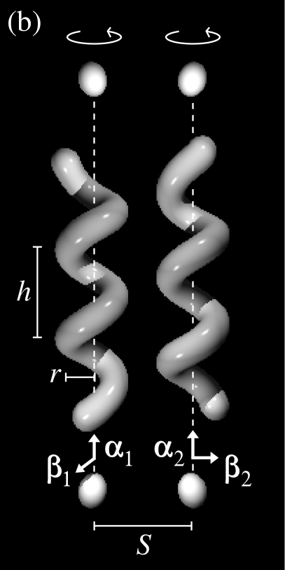
Figure 1: Visualization of the helix geometry used in the simulations (here with a phase difference of $\pi/2$). (a) All beads of one helix are connected ridigly with each other. (b) For the sake of clarity, the beads are “smeared” out along the helix. The top and bottom beads are anchored in harmonic traps. The illustrated helices are in their equilibrium positions (i.e., in the absence of driving torques).

The model is introduced in detail in Sec. 2. Then, symmetry properties of the dynamic quantities are derived in Sec. 3. The numerical simulations of the helix dynamics are presented in detail in Sec. 4, where we analyze the data for phase synchronization, in particular with respect to the anchoring strength of the terminal beads. Finally, we conclude in Sec. 5 discussing the role of the harmonic traps and the flexibility which they create.

2 Model

We consider two identical helices built of equal-sized beads [Fig. 1(a)] that are connected with each other by (virtual) rigid bonds. Thus, the helices cannot deform elastically. The centers of the beads are aligned along the backbone of the helix, with equal distances between successive beads.

To describe the dynamics of the helices, we introduce body-fixed coordinate axes, given by the orthonormal vectors $\vec{\alpha}_{i}$, $\vec{\beta}_{i}$, and $\vec{\alpha}_{i}\times\vec{\beta}_{i}$ ($i=1,2$). The axis of a helix is represented by $\vec{\alpha}_{i}$, and the orientation of the perpendicular vector $\vec{\beta}_{i}$ shall describe the phase of the helix, i.e., the rotation about its own axis [Fig. 1(b)]. We define the phase angles $\phi_{i}$ by the projection of $\vec{\beta}_{i}$ into the $xy$ plane (Fig. 2). The angle between $\vec{\alpha}_{i}$ and the $z$ axis is the tilt angle $\theta_{i}$.

[width=0.45]angles

Figure 2: The helix axis $\vec{\alpha}_{i}$ is tilted by the angle $\theta_{i}$ against the $z$ direction. The phase $\phi_{i}$ measures the angle between the $xy$-plane projection of the phase vector $\vec{\beta}_{i}$ and the $x$ axis.

The centers of mass of the helices are denoted by $\vec{x}_{i}$. The positions of the individual beads are then given by

$$\bar{\vec{x}}_{i}^{\nu}=\vec{x}_{i}+\xi_{1}^{\nu}\vec{\alpha}_{i}+\xi_{2}^{\nu}\vec{\beta}_{i}+\xi_{3}^{\nu}\vec{\alpha}_{i}\times\vec{\beta}_{i}$$ (1)

with the internal coordinates

$$\begin{array}[]{c}\displaystyle\xi_{1}^{\nu}=\frac{h}{m}\left(\nu-\frac{nm-1}{2}\right)\,,\\[17.07164pt] \displaystyle\xi_{2}^{\nu}=r\cos\frac{2\pi}{m}\,\nu\,,\quad\displaystyle\xi_{3}^{\nu}=r\sin\frac{2\pi}{m}\,\nu\,,\end{array}$$ (2)

where $r$ is the radius of the helix and $h$ its pitch. The bead index $\nu$ runs from $0$ to $nm-1$ for each helix, with $m$ being the number of beads per winding and $n$ the number of windings.

[width=0.65]symmetry_z         

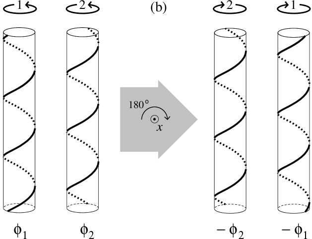
Figure 3: Rotation of the two-helix system by $180^{\circ}$ about the $z$ axis (a) and about the $x$ axis (b). The circular arrows (indexed with $i=1,2$) on top of the helices denote that the respective helix is driven with torque $T_{i}$ and rotates with velocity $\omega_{i}$ in the indicated direction. The tubes are drawn as guide to the eye.

The helices are driven by constant and equal torques that are always parallel to the respective helix axis, i.e., the torques are given by $D\vec{\alpha}_{i}$ with a fixed parameter $D$. Note that the assumption of a constant torque agrees with experimental studies of real flagellar motors ber03 ; man80 , as we have already mentioned in our introductory remarks. To “fix” the helices in space, we attach single beads at the top and bottom end of each helix axis (Fig. 1) and anchor them in harmonic traps with equal force constants $K$. In equilibrium, both helix axes are parallel, and their center-to-center distance is $S$. If one of the anchoring beads is displaced by $\Delta\bar{\vec{x}}_{i}^{\sigma}$ (where the index $\sigma$ refers to “top” or “bottom”) relative to the center of the respective harmonic trap, the restoring single-particle force is

$$\bar{\vec{F}}_{i}^{\sigma}=-K\Delta\bar{\vec{x}}_{i}^{\sigma}\,.$$ (3)

Finally, the total center-of-mass forces and torques acting on the rigid helices are

$$\begin{array}[]{l}\vec{F}_{i}=\sum\limits_{\sigma}\bar{\vec{F}}_{i}^{\sigma}\quad(\text{with}\ \sigma=\text{top, bottom})\,,\\[11.38109pt] \vec{T}_{i}=D\vec{\alpha}_{i}+\sum\limits_{\sigma}(\bar{\vec{x}}_{i}^{\sigma}-\vec{x}_{i})\times\bar{\vec{F}}_{i}^{\sigma}\,.\end{array}$$ (4)

In the regime of low Reynolds numbers, the flow of an incompressible fluid with viscosity $\eta$ obeys the quasi-static Stokes or creeping flow equations $\eta\nabla^{2}\vec{u}-\nabla p=\vec{0}$ and $\nabla\cdot\vec{u}=0$ dho96 ; bre63/64 , where $\vec{u}$ is the flow field and $p$ the hydrodynamic pressure. We assume the flow to vanish at infinity and impose stick boundary conditions on the surfaces of all particles suspended in the fluid. The resulting flow field then couples the motion of the particles to each other. Due to the linearity of the Stokes equations, their translational and rotational velocities, $\vec{v}_{i}$ and $\vec{\omega}_{i}$, depend linearly on all external forces and torques, $\vec{F}_{j}$ and $\vec{T}_{j}$ dho96 ; bre63/64 :

$$\begin{array}[]{l}\vec{v}_{i}=\sum\limits_{j}\boldsymbol{\mu}_{ij}^{\text{tt}}\vec{F}_{j}+\sum\limits_{j}\boldsymbol{\mu}_{ij}^{\text{tr}}\vec{T}_{j}\,,\\[11.38109pt] \vec{\omega}_{i}=\sum\limits_{j}\boldsymbol{\mu}_{ij}^{\text{rt}}\vec{F}_{j}+\sum\limits_{j}\boldsymbol{\mu}_{ij}^{\text{rr}}\vec{T}_{j}\,.\end{array}$$ (5)

Each of the mobilities $\boldsymbol{\mu}_{ij}^{\text{tt}}$, $\boldsymbol{\mu}_{ij}^{\text{tr}}$, $\boldsymbol{\mu}_{ij}^{\text{rt}}$, and $\boldsymbol{\mu}_{ij}^{\text{rr}}$ is a $3\times 3$ tensor, which couples the translations (superscript t) and rotations (superscript r) of particles $i$ and $j$. They depend on the current spatial configuration of all suspended particles. Since this dependence is highly nonlinear, they have to be calculated numerically.

In our simulations, we use the numerical library hydrolib hin95 which yields the full set of mobility tensors for a given configuration of equal-sized spherical particles (based on the multipole expansion method). It implicitly accounts for (virtual) rigid bonds that keep the relative positions of the single beads in a rigid cluster fixed. Thus, hydrolib calculates an effective mobility matrix for the coupled center-of-mass translations and rotations, i.e., the indices $i$ and $j$ in Eq. (5) now refer to rigid clusters instead of individual beads (for details, see Ref. hin95 ).

Therefore, with the forces and torques given in Eq. (4), we directly obtain the linear and angular velocities of the helices. The translational motion of the centers of mass is then governed by

$$\dot{\vec{x}}_{i}=\vec{v}_{i}\,,$$ (6)

where the dot means time derivative. The rotational motion of the helix axes $\vec{\alpha}_{i}$ and the phase vectors $\vec{\beta}_{i}$ follows from

$$\begin{array}[]{l}\dot{\vec{\alpha}}_{i}=\vec{\omega}_{i}\times\vec{\alpha}_{i}\,,\\[5.69054pt] \dot{\vec{\beta}}_{i}=\vec{\omega}_{i}\times\vec{\beta}_{i}\,.\end{array}$$ (7)

We integrate these equations in time by applying a second-order Runge-Kutta scheme (also known as Heun algorithm) kloe99 . Note that the mobility matrices have to be evaluated at each time step since the positions and orientations of the helices change.

While the trap constant $K$ was varied to study the influence of the anchoring strength on the helix dynamics, the driving torque $D$ was kept fixed since it merely sets the time scale (given by the rotational frequency $\omega_{0}$ of an isolated helix). The time steps of the numerical integration where chosen to correspond to roughly 1/360th of a revolution of a single helix.

The geometry of the two helices is shown in Fig. 1. Their backbones have a radius of $r=2.0a$ and a pitch of $h=6.0a$, where $a$ is the bead radius. The number of windings is $n=3$, and the number of beads per winding is $m=5$. The distance between the anchoring beads and the helix is the same as the pitch $h$. The equilibrium separation of the helices, i.e., the distance of the upper/lower anchoring traps, is $S=7.0a$. Note that the calculation of the mobility matrix is the most time consuming part in the simulations. Therefore, we had to restrict the number of beads in one helix. Furthermore, we will only present results for the set of parameters just introduced and concentrate on the essential variable, namely the trap stiffness $K$.

3 Symmetry considerations

Consider for the moment two helices whose axes are completely fixed in space, i.e., translation and tilt are prevented by appropriate forces and torques. In this case, the only remaining degrees of freedom are rotations about the axes of the helices. They are described by the phase angles $\phi_{i}$ and the angular velocities $\dot{\phi}_{i}=\omega_{i}$. We introduce the phase difference $\chi=\phi_{2}-\phi_{1}$ as the phase of the right helix relative to the left helix, when viewed as in Fig. 3(a,b) (left part). According to Eq. (5), the rotational velocities $\omega_{i}$ are functions of the phase angles $\phi_{i}$ since the mobility tensors depend on the spatial configuration. As the helices are driven by the same torques $T_{i}=D$ about their axes, the synchronization rate is given by

$$\dot{\chi}=\omega_{2}(\phi_{1},\phi_{2})-\omega_{1}(\phi_{1},\phi_{2})=\mu(\phi_{1},\phi_{2})D\,,$$ (8)

where the effective mobility $\mu$ is $2\pi$-periodic in $\phi_{i}$. We choose this careful definition because we now want to derive symmetry properties of $\mu$.

We use the fact that the dynamics of the two-helix system must not change under arbitrary rotations of the whole geometry since the surrounding fluid is isotropic. By applying the two operations illustrated in Fig. 3, we create new configurations with left and right helices whose known dynamics we use to infer properties of the mobility $\mu$.

In the first case, we rotate the two-helix system by $180^{\circ}$ about the $z$ axis, as illustrated in Fig. 3(a). The velocities of the left and right helix are exchanged, i.e., $\omega_{1}\leftrightarrow\omega_{2}$ and thus $\dot{\chi}\to-\dot{\chi}$. On the other hand, the phase angles of the new left and right helix are, respectively, $\phi_{2}+\pi$ and $\phi_{1}+\pi$. Combining both statements, Eq. (8) yields

$$\mu(\phi_{2}+\pi,\phi_{1}+\pi)=-\mu(\phi_{1},\phi_{2})\,.$$ (9)

If the phases of the helices differ by $\pi$ ($\phi_{2}=\phi_{1}+\pi$), one therefore obtains $\mu(\phi_{1},\phi_{1}+\pi)=-\mu(\phi_{1},\phi_{1}+\pi)=0$ or

$$\dot{\chi}=0\quad\text{for}\quad\chi=\pi\,,$$ (10)

i.e., the synchronization speed vanishes for any $\phi_{1}$ whenever $\phi_{2}-\phi_{1}=\pi$.

Let us now rotate the two-helix system by $180^{\circ}$ about the $x$ axis [Fig. 3(b)]. Then the velocities of the left and right helix are exchanged and reversed, i.e., $\omega_{1}\leftrightarrow-\omega_{2}$, and the synchronization speed $\dot{\chi}=-\omega_{1}-(-\omega_{2})=\omega_{2}-\omega_{1}$ stays the same. On the other hand, the angles transform as $\phi_{1}\leftrightarrow-\phi_{2}$, and the driving torques are reversed, i.e., $D\to-D$. Again, combining both statements, Eq. (8) yields $\mu(-\phi_{2},-\phi_{1})(-D)=\mu(\phi_{1},\phi_{2})D$, and thus

$$\mu(-\phi_{2},-\phi_{1})=-\mu(\phi_{1},\phi_{2}).$$ (11)

For helices of infinite length, the dynamics can only depend on the phase difference $\chi$ and not on the single phases $\phi_{i}$. This is obvious since a phase shift of both helices is equivalent to a translation along the helix axes, which does not change the dynamics. Hence, Eq. (11) reads $\mu(\chi)=-\mu(\chi)=0$, i.e., for parallel helices of infinite length, the synchronization rate $\dot{\chi}=\mu(\chi)D$ vanishes for any phase difference $\chi$, and therefore, they do not synchronize towards $\chi=0$ foot:kin_rev .

4 Synchronization

We now study the rotational dynamics of two helices whose terminal beads are anchored in harmonic traps of finite strength, as introduced in Sec. 2. Thus, the helices can be shifted and tilted, and their axes undergo a precession-like motion while each helix itself is rotating about its respective axis. The orientations of the helices in space are described by the vectors $\vec{\alpha}_{i}$ and $\vec{\beta}_{i}$ [see Fig. 1(b)] and the corresponding angles $\theta_{i}$ and $\phi_{i}$, as defined in Fig. 2.

Figure 4 shows the phase difference $\chi=\phi_{2}-\phi_{1}$ for two trap stiffnesses $K$ as a function of a reduced time $\tau(K)$, to be defined below. Starting with $\chi$ slightly smaller than $\pi$, the phase difference decreases continuously (with steepest slope at $\chi=\pi/2$) and finally approaches zero, i.e., the two helices do indeed synchronize their phases. The simulations reveal that the dynamics does not depend significantly on the phases $\phi_{i}$ themselves, but is predominantly determined by the phase difference $\chi$. Note that this feature may be expected since the dynamics of parallel helices of infinite length can only depend on $\chi$ as explained in Sec. 3. To be concrete, we observe that the rotational velocities $\dot{\phi}_{i}$ undergo oscillations of only about 1% around a mean value during one rotational period. Their amplitude does not depend on the trap stiffness $K$, i.e., the oscillations originate from the slight dependence on the phases themselves (and not from the precession of the axes). Therefore, starting with different values for $\phi_{i}$ but the same value of $\chi$ yields the same curve (except for differences in the small oscillations illustrated in the insets of Fig. 4).

Figure 4: Synchronization of the helix rotations. The phase difference of the two helices tends towards zero, starting from $\chi$ slightly smaller than $\pi$. The symbols are simulation data at two different trap strengths (values of $K$ in units of $D/a$). For clarity, not every data point is plotted. The solid line shows the master curve of Eq. (12). The insets enlarge the small oscillations at $\chi\approx 0$ and $\pi$ (here for the case $K=0.05\,D/a$, but the amplitudes do not depend strongly on $K$). Note that the scaling of the two insets is the same.

The mean rotational velocities, averaged over one rotational period, increase during the synchronization process from about $0.92\omega_{0}$ at $\chi\approx\pi$ to about $0.95\omega_{0}$ at $\chi\approx 0$ (Fig. 5). Thus, the hydrodynamic drag acting on the helices is minimized during phase synchronization (see also Ref. kim04b ). Since the torques are constant, the dissipation rate $\sum_{i}\vec{T}_{i}\cdot\vec{\omega}_{i}$ is maximized. This observations agrees with the interesting fact that the Stokes equations can be derived from a variational principle where one searches for an extremum of the dissipated energy $\int\sigma_{ij}A_{ij}d^{3}r$ ($\sigma_{ij}$ is the stress tensor and $A_{ij}$ the symmetrized velocity gradient) under the constraint that the fluid is incompressible lam72 ; fin72 . The pressure enters via the Lagrange parameter associated with the constraint.

Figure 5: Mean rotational velocities, averaged over one revolution (in units of the rotational frequency $\omega_{0}$ of an isolated helix). The oscillations about the mean value are of the order of a few percent, they decrease slightly during the synchronization process. The example shown is for trap strength $K=0.15\,D/a$.

In Sec. 3, we showed for fixed parallel helices, based on pure symmetry arguments, that their synchronization rate vanishes for a phase difference of $\chi=\pi$ [see Eq. (10)]. In that case, the two-helix configuration is symmetric with respect to a rotation by $180^{\circ}$ about the $z$ axis [see Fig. 3(a)]. Our reasoning of Sec. 3 can be extended to the case of non-parallel helix axes, as long as the same symmetry is preserved. However, $\chi=\pi$ does not correspond to a stable state. Starting with $\chi$ marginally smaller than $\pi$, the system tends towards phase difference zero. The simulation with $K=0.05$ in Fig. 4 was launched, e.g., at $\chi=0.994\pi$ with both helices in equilibrium position and orientation, as shown in Fig. 1.

Figure 6: Synchronization speed (taken at a relative phase $\chi\approx\pi/2$, as illustrated in the inset) as a function of inverse trap strength $K^{-1}$. The frequency scale $\omega_{0}$ for the synchronization speed is the angular velocity of an isolated helix. The symbols indicate values extracted from simulations at different $K$. The dashed line is an empirical fit (see text).

On the other hand, the synchronized state $\chi=0$ is stable against small perturbations since configurations with $\chi$ between 0 and $-\pi$ synchronize towards zero phase difference, too. This was checked by simulations, but can also be derived from Eq. (9). The corresponding rotation of Fig. 3(a) creates new left and right helices with a change in sign for $\chi$ and $\dot{\chi}$ relative to the original helices which explains our statement. Furthermore, starting a simulation with exactly $\chi=0$, the helices remain synchronized on average (i.e., $\langle\chi\rangle=0$), but there are still small oscillations as illustrated in the lower right inset in Fig. 4 for the case where both helices started in equilibrium position and orientation.

Averaging over small oscillations, we find that the resulting smoothed curves for the phase difference $\chi$ obey an empirical law of the form

$$\chi(\tau)=\frac{\pi}{2}(1-\tanh\tau)\,,$$ (12)

where

$$\tau(K)=\frac{2}{\pi}\,(t-t_{\pi/2})\left|\frac{\text{d}\chi}{\text{d}t}\right|_{t=t_{\pi/2}}$$ (13)

is the reduced time, already mentioned above, and $t_{\pi/2}$ denotes the time where $\chi=\pi/2$, i.e., the location of the inflection point. Its slope $|\text{d}\chi/\text{d}t|_{t=t_{\pi/2}}$ depends on the trap stiffness $K$ and so does $\tau$. As Fig. 4 strikingly reveals, this law works very well. By plotting the phase difference $\chi$ versus the reduced time $\tau(K)$, the curves collapse on the master curve given by Eq. (12). Since the dynamics at low Reynolds numbers is completely overdamped, we expect this law to follow from a differential equation which is of first order in time. Taking the first derivative of Eq. (12) with respect to $\tau$, we find that $\chi(\tau)$ obeys the nonlinear equation $\dot{\chi}(\tau)=(2/\pi)\chi(\tau)[\pi-\chi(\tau)]$, known as the Verhulst equation and originally proposed to model the development of a breeding population arf95 . However, it is not clear how to derive this equation from first principles in our case.

Figure 7: Tilt of the left and right helix axis for $K=0.05$ and $0.15$ as a function of reduced time $\tau$. The fast periodic oscillations of the tilt angles $\theta_{i}$ yield the black bands since they cannot be resolved on the time scale used here. The insets visualize the precession of the helix axes by showing the tip of the vectors $\vec{\alpha}_{i}$ (at $\chi\approx\pi/2$). From the outer to the inner “circular” orbit, the trap stiffness assumes the values $K=0.05$, 0.1, 0.15, and 1.0 (in units of $D/a$).

An important result is that the speed of the synchronization process decreases with increasing trap stiffness $K$. The values plotted in Fig. 6 for different $K^{-1}$ are the slopes $|\text{d}\chi/\text{d}t|_{t=t_{\pi/2}}$ extracted from simulation data at the inflection point with a relative phase of $\chi\approx\pi/2$. The curve in Fig. 6 can be extrapolated by the analytic form $c_{1}\tanh c_{2}K^{-1}$ (dashed curve), where the fit parameters assume the values $c_{1}=3.67\cdot 10^{-3}\omega_{0}$ and $c_{2}=0.0685\,D/a$. In the limit of infinite trap strength, i.e., for $K^{-1}\to 0$, the synchronization speed clearly tends towards zero, i.e., an infinitely strong anchoring of the helix axes does not allow for phase synchronization.

In Fig. 7, we illustrate how the tilt angles $\theta_{i}$ (for their definition, see Fig. 2) vary during the synchronization process. The mean tilt angle as well as the amplitude of its periodic oscillations decrease when the phase difference approaches zero. Obviously, the dynamics of the helices depends on the stiffness of the harmonic anchoring of the top and bottom terminal beads. In a weaker trap, the tilt of the helix axes out of equilibrium is more pronounced compared to a stronger trap. The insets in Fig. 7 track the precession-like motions of the helix axes. The stronger the trap, the smaller the radius of the “orbit” or the tilt angle. [Since the simulations were started with both axes aligned along their equilibrium direction, the trajectories $(\alpha_{ix},\alpha_{iy})$ first move radially away from the origin and then enter the “precession orbit”.]

In real flagellar motors, the torques on the two helical filaments are not exactly the same. To test whether the phenomenon of synchronization still occurs, we now consider slightly different driving torques for the two helices. The first helix is still driven with torque $D$, while the second helix is driven with $D+\Delta D$ ($\Delta D>0$). We observe that, for torque differences $\Delta D$ below a critical value $\Delta D_{\text{c}}$, the two helices indeed synchronize towards a phase difference $\chi_{\infty}=\chi(t\to\infty)$, which, in general, is not zero. The results are shown in Fig. 8, where we plot $1-\chi_{\infty}/\frac{\pi}{2}$ as a function of $\Delta D/\Delta D_{\text{c}}$. With increasing $\Delta D$, the phase lag $\chi_{\infty}$ increases from zero to $\pi/2$. For $\Delta D>\Delta D_{\text{c}}$, there is no synchronization, and the phase difference grows continuously. Note that the reduced critical torque difference $\Delta D_{\text{c}}/D=3.22\cdot 10^{-3}$ corresponds to the reduced frequency difference $\dot{\chi}/\omega_{0}=(\omega_{2}-\omega_{1})/\omega_{0}$ observed at $\chi=\pi/2$ for equal torques ($\Delta D=0$). At the critical torque difference, the helices synchronize towards a phase lag of $\chi=\pi/2$. This means that $\Delta D_{\text{c}}$ just compensates the difference in the effective mobilities of the two helices, which is largest for $\chi=\pi/2$; thus the helices rotate with the same speed.

Figure 8: Phase difference $\chi_{\infty}$ (plotted as $1-\chi_{\infty}/\frac{\pi}{2}$) of the synchronized state as a function of the torque difference $\Delta D$. The phase difference increases from $\chi_{\infty}=0$ to $\pi/2$ (or $1-\chi_{\infty}/\frac{\pi}{2}$ decreases from 1 to 0) with increasing torque difference. For $\Delta D>\Delta D_{\text{c}}$, there is no synchronization.

At the end, we mention that all results presented here refer to helices whose rotational direction is given in Fig. 1(b). Reversing the direction of rotation does not change the dynamics of the two-helix system since this can also be achieved by the operation shown in Fig. 3(b) that does not change the synchronization speed.

5 Conclusions

We have reported that two rigid helices whose terminal beads are anchored in harmonic traps and which are driven by equal torques synchronize to zero phase difference. The effect is robust, i.e., if the torques are unequal, the helices synchronize to a non-zero phase lag below a critical torque difference. This agrees with observations in Ref. kim03 where the helices do not bundle if the motor speeds are sufficiently different. Increasing the stiffness of the anchoring traps, decreases the synchronization rate. We attribute this to the jiggling motion of the two helix axes which is more and more restrained.

In the limit of infinite trap strength, our results are consistent with recent work based on slender-body theory for two rigid helices kim04b . If the helices are prevented from translation and their axes are always kept parallel, then there is no synchronization possible. Therefore, we conclude that the additional degree of freedom due to the finite anchoring of the helix axis, i.e., the jiggling motion, is essential to enable phase synchronization in our model.

At a first glance, our model might appear too artificial for describing the hydrodynamic coupling of flagella. However, our results clearly indicate that some kind of flexibility is essential to allow for phase synchronization. In reality, this flexibility might have its origin in elastic deformations of the rotating flagella. Therefore, the next step is to make the flexural and torsional stiffness of the helices in our model finite.

The helix used in our numerical investigation with radius $r=2a$ and pitch $h=6a$ is far from the values of a real bacterial filament with $r=20a$ and $h=200a$ where $a$ is now half the filament diameter. We have tried different paths in the parameter space $(r,h)$ to connect both cases, i.e, our “fat” helix and the real slender helix. We observe that making the helix more slender decreases the synchronization speed in units of $\omega_{0}$. This makes sense since the induced flow from the rotation of slender helices is smaller. To reduce computer time, we extrapolated the synchronization speeds for different paths in the $(r,h)$ space towards the real helical flagellum and found that the speed is reduced by a factor of 60 to 70 compared to the results reported in this article. At a first glance this seems to be a discouraging result. However, from preliminary results of helices with finite bending and torsional flexibility, we know already that these factors considerably increase the synchronization speed so that it will be of biological relevance.

Furthermore, we made a comparison of the resistance matrix of a real flagellum modeled by a sequence of spheres with resistive force theory as summarized, e.g., in Ref. joh79 . We found that for motion and rotation along the helix axis, the single matrix elements differ by less than a factor of two. This convinces us that modelling a flagellum with the method presented in this article is appropriate. For our fat helix, however, the deviations are larger since the filament is relatively thick compared to radius and pitch of the helix. So the conditions for the validity of resistive force theory are not satisfied so well.

We also checked whether it is important if the helices are forced to stay at their position or if they are allowed to propel themselves. This was done by letting the helices move along the $z$ axis but still keeping them in harmonic traps along the $x$ and $y$ direction. However, we did not see a significant difference in the dynamics of the synchronization process compared to the results presented in this work.

As a final remark, we point out that the following general mechanism may exist in systems of low Reynolds numbers: Synchronizing the motions of some objects via hydrodynamic interactions needs some kind of “flexibility”. If the motions of the objects are constrained too much, synchronization cannot occur. We have observed a similar behavior for particles circling in a toroidal harmonic trap and driven by a constant tangential force rei04 . After some transition regime, the particles reach a synchronized state where they perform a periodic limit cycle. We observe that for increasing trap stiffness, i.e., for decreasing oscillations along the radial direction, the time to reach this limit cycle increases.

- (1) H.C. Berg, Nature 245, 380 (1973).
- (2) R.M. Macnab, in Escherichia coli and Salmonella typhimurium, edited by F.C. Neidhardt (Am. Soc. Microbiol., Washington DC, 1987), p. 70.
- (3) L. Turner, W.S. Ryu, H.C. Berg, J. Bacteriol. 182, 2793 (2000). Movies of swimming E. coli can be found at http://webmac.rowland.org/labs/bacteria/movies_ecoli.html.
- (4) H.C. Berg, Annu. Rev. Biochem. 72, 19 (2003).
- (5) H.C. Berg, E. coli in Motion (Springer, New York, 2004).
- (6) M.D. Manson, P.M. Tedesco, H.C. Berg, J. Mol. Biol. 138, 541 (1980).
- (7) R.M. Macnab, Proc. Natl. Acad. Sci. USA 74, 221 (1977).
- (8) M.J. Kim, J.C. Bird, A.J. Van Parys, K.S. Breuer, T.R. Powers, Proc. Natl. Acad. Sci. USA 100, 15481 (2003). A movie of the bundling sequence of two rotating (macroscopic) helices can be found at http://www.pnas.org/cgi/content/full/2633596100/DC1.
- (9) M.J. Kim, M.J. Kim, J.C. Bird, J. Park, T.R. Powers, K.S. Breuer, Exp. Fluids 37, 782 (2004).
- (10) R.M. Macnab, M.K. Ornston, J. Mol. Biol. 112, 1 (1977).
- (11) E.M. Purcell, Am. J. Phys. 45, 3 (1977).
- (12) J.K.G. Dhont, An Introduction to Dynamics of Colloids (Elsevier, Amsterdam, 1996).
- (13) G. Taylor, Proc. R. Soc. Lond. A 209, 447 (1951).
- (14) M.C. Lagomarsino, B. Bassetti, P. Jona, Eur. Phys. J. B 26, 81 (2002).
- (15) M.C. Lagomarsino, P. Jona, B. Bassetti, Phys. Rev. E 68, 021908 (2003).
- (16) S. Gueron, K. Levit-Gurevich, Proc. Natl. Acad. Sci. USA 96, 12240 (1999).
- (17) M.J. Kim, T.R. Powers, Phys. Rev. E 69, 061910 (2004).
- (18) H. Brenner, Chem. Eng. Sci. 18, 1 (1963); 19, 599 (1964).
- (19) K. Hinsen, Comput. Phys. Commun. 88, 327 (1995).
- (20) P.E. Kloeden, E. Platen, Numerical Solution of Stochastic Differential Equations (Springer, Berlin, 1999).
- (21) The same result with similar methods was obtained by Kim and Powers in Ref. kim04b . They use the concept of kinematic reversibility of Stokes flow that manifests itself, e.g., in Eq. (8). That means, to arrive at Eq. (11), we use this concept when the torque on the helices is reversed.
- (22) H. Lamb, Hydrodynamics (Cambridge University Press, London, 1975).
- (23) B.A. Finlayson, The Method of Weighted Residulas and Variational Principles (Academic Press, New York, 1972).
- (24) G.B. Arfken, H.J. Weber, Mathematical Methods for Physicists (Academic Press, San Diego, 1995).
- (25) R.E. Johnson, C.J. Brokaw, Biophys. J. 25, 113 (1979).
- (26) M. Reichert, H. Stark, J. Phys.: Condens. Matter 16, S4085 (2004).