New mean-field theory of the $tt^{\prime}t^{\prime\prime}J$ model applied to the high-T_c superconductors

Abstract

We introduce a new mean-field approach to the $tt^{\prime}t^{\prime\prime}J$ model that incorporates both electron-like quasiparticle and spinon excitations as suggested by some experiments and numerical studies. It leads to a mean-field phase diagram which is consistent with that of hole and electron doped cuprates. Moreover, it provides a framework to describe the observed evolution of the electron spectral function from the undoped insulator to the overdoped Fermi metal for both hole and electron doping. The theory also provides a new non-BCS mechanism leading to superconductivity.

The evolution of the electronic structure from the undoped antiferromagnetic (AF) insulator to the overdoped metallic state of cuprates is a long standing problem. The plethora of anomalous behavior displayed by these materials is particularly striking in hole underdoped samples, for which both experimental DS0373 ; ZY0401 ; RS0301 ; KS0318 ; IK0204 ; YZ0301 and numerical TS0009 ; LL0301 ; R0402 evidence suggests a dichotomy of the electronic excitations: excitations around the nodal points [$\boldsymbol{k}=(\pm\tfrac{\pi}{2},\pm\tfrac{\pi}{2})$] are well described as Landau’s quasiparticles while those near the antinodal points [$\boldsymbol{k}=(\pi,0),\,(0,\pi)$] show no signs of quasiparticle-like behavior. Some experimental KRUSIN and numerical TS0009 ; LL0301 ; R0402 ; ME9916 studies relate the absence of quasiparticles close to the antinodal points to the presence of excitations that only carry spin.

In order to account for the aforementioned nodal-antinodal dichotomy, in this letter, a new mean-field (MF) approach to the $tt^{\prime}t^{\prime\prime}J$ model is introduced which describes the low energy physics in terms of spinons and doped carriers. Spinons are electrically neutral fermions describing spin-1/2 excitations. In the $tt^{\prime}t^{\prime\prime}J$ model double occupancy is prohibited and the doped carriers correspond to the removal of a lattice spin, which inserts a unit charge and a spin-1/2 in the system. Doped carriers are holes in the hole doped (HD) regime and electrons in the electron doped (ED) regime. For ease of speaking, below we refer to the doped carriers as dopons, which are spin-1/2 charged fermions. We show that the new MF approach leads to a MF phase diagram that resembles the one of HD and ED cuprates. It also accounts for the doping evolution of the electronic structure, as seen by ARPES, in both HD and ED samples.

We start with the 2D $tt^{\prime}t^{\prime\prime}J$ Hamiltonian

$$H_{tJ}=J\!\!\!\!\!\sum_{\langle ij\rangle\in NN}\!\!\!\!\!\bm{S}_{i}.\bm{S}_{j}-\sum_{\langle ij\rangle,\sigma}t_{ij}\mathcal{P}\left(c_{i,\sigma}^{\dagger}c_{j,\sigma}+h.c.\right)\mathcal{P}$$ (1)

where $t_{ij}=t,t^{\prime},t^{\prime\prime}$ for first, second and third nearest neighbor (NN) sites and $\mathcal{P}$ projects out doubly occupied sites. The $tJ$ model on-site Hilbert space, $\{\left|\uparrow\right\rangle,\left|\downarrow\right\rangle,\left|0\right\rangle\}$, includes states with either one or zero spin-$\tfrac{1}{2}$ objects.

To obtain the new MF theory we start with an enlarged on-site Hilbert space $\{\left|\uparrow\!\!0\right\rangle,\left|\downarrow\!\!0\right\rangle,\left|\uparrow\uparrow\right\rangle,\left|\uparrow\downarrow\right\rangle,\left|\downarrow\uparrow\right\rangle,\left|\downarrow\downarrow\right\rangle\}$ which contains either one or two spin-$\tfrac{1}{2}$ objects. The states $\left|\uparrow\!\!0\right\rangle$, $\left|\downarrow\!\!0\right\rangle$ and the local singlet state $\tfrac{1}{\sqrt{2}}(\left|\uparrow\downarrow\right\rangle-\left|\downarrow\uparrow\right\rangle)$ are the physical states that map onto the states $\left|\uparrow\right\rangle$, $\left|\downarrow\right\rangle$ and the vacancy state $\left|0\right\rangle$, respectively, in the $tJ$ model on-site Hilbert space. The on-site triplet states, such as $\tfrac{1}{\sqrt{2}}(\left|\uparrow\downarrow\right\rangle+\left|\downarrow\uparrow\right\rangle)$, are unphysical. We also introduce the fermionic representation for the first spin (the lattice spin), $\bm{S}_{i}=\tfrac{1}{2}f_{i}^{\dagger}\bm{\sigma}f_{i}$, and the second spin (the doped spin), $\tfrac{1}{2}d_{i}^{\dagger}\bm{\sigma}d_{i}$, where $\bm{\sigma}$ are the Pauli matrices. Here, the spinors $f_{i}^{\dagger}\equiv[f_{i,\uparrow}^{\dagger}f_{i,\downarrow}^{\dagger}]$ and $d_{i}^{\dagger}\equiv[d_{i,\uparrow}^{\dagger}d_{i,\downarrow}^{\dagger}]$ are the spinon and the dopon creation operators on site $i$. Then, the Hamiltonian $H_{tJ}^{enl}=H_{enl}^{t}+H_{enl}^{J}$, where

$$H_{enl}^{t} = \sum_{\langle ij\rangle}\frac{t_{ij}}{2}\widetilde{\mathcal{P}}\left[\left(d_{i}^{\dagger}\bm{\sigma}d_{j}\right).\left(i\bm{S}_{i}\times\bm{S}_{j}-\frac{\bm{S}_{i}+\bm{S}_{j}}{2}\right)+\right.$$

$$\left.\quad\quad\quad\quad\quad+\frac{1}{4}d_{i}^{\dagger}d_{j}+d_{i}^{\dagger}d_{j}\bm{S}_{i}.\bm{S}_{j}+h.c.\right]\widetilde{\mathcal{P}}$$

$$H_{enl}^{J} = J\!\sum_{\langle ij\rangle\in NN}\!\bm{S}_{i}.\bm{S}_{j}\,\widetilde{\mathcal{P}}\left(1-d_{i}^{\dagger}d_{i}\right)\left(1-d_{j}^{\dagger}d_{j}\right)\widetilde{\mathcal{P}}\ ,$$ (2)

equals $H_{tJ}$ in the physical Hilbert space and does not connect the physical and the unphysical sectors of the Hilbert space. $H_{enl}^{t}$ is such that only local singlet states hop between different lattice sites whereas the unphysical local triplet states have no kinetic energy. Therefore, the dynamics included in $H_{enl}^{t}$ effectively implements the local singlet constraint. The enlarged on-site Hilbert space contains at most one dopon. Hence, in (2), we introduce the projection operator $\widetilde{\mathcal{P}}=\prod_{i}(1-d_{i,\uparrow}^{\dagger}d_{i,\uparrow}d_{i,\downarrow}^{\dagger}d_{i,\downarrow})$ which enforces the no double occupancy constraint for the $d$-fermion. By definition, the total number of dopons in the system equals the number of doped carriers. We are mostly interested in the low doping regime and, thus, below we drop the projection operators $\widetilde{\mathcal{P}}$ in $H_{tJ}^{enl}$.

The Hamiltonian $H^{enl}_{tJ}$ is a sum of terms with up to six fermion operators. In the following we replace some multiple-fermion operators by their average so that the resulting MF Hamiltonian is quadratic in the operators $f^{\dagger}$, $f$, $d^{\dagger}$ and $d$, and describes the hopping, pairing and mixing of spinons and dopons.

The exchange Hamiltonian $H_{enl}^{J}$ is decoupled by means of the d-wave ansatz WL9603 and becomes $-\tfrac{3\tilde{J}}{8}\sum_{\langle ij\rangle\in NN}[\chi f_{i}^{\dagger}f_{j}+(-)^{j_{y}-i_{y}}\Delta(f_{i\uparrow}^{\dagger}f_{j\downarrow}^{\dagger}-f_{i\downarrow}^{\dagger}f_{j\uparrow}^{\dagger})+h.c.]+a_{0}\sum_{i}(f_{i}^{\dagger}f_{i}-1)$ where $\chi$ and $\Delta$ are the spinon bond and pairing MFs and $a_{0}$ is the Lagrange multiplier enforcing $\bigl{<}f_{i}^{\dagger}f_{i}\bigr{>}=1$. Also, $\tilde{J}=(1-x)^{2}J$, where we introduce the doping density $x=\bigl{<}d_{i}^{\dagger}d_{i}\bigr{>}$.

We now consider the hopping Hamiltonian $H_{enl}^{t}$. Since the effective hopping amplitude of one hole in an AF background is renormalized by spin fluctuations, KL8980 we replace the bare $t$, $t^{\prime}$ and $t^{\prime\prime}$ by the effective hopping parameters $t_{1}$, $t_{2}$ and $t_{3}$ which are determined phenomenologically. The terms $[(d_{i}^{\dagger}\bm{\sigma}d_{j}).(i\bm{S}_{i}\times\bm{S}_{j})]$ and $(d_{i}^{\dagger}d_{j}\bm{S}_{i}.\bm{S}_{j})$ in $H_{enl}^{t}$ are the sum of operators like $d_{i,\alpha}^{\dagger}d_{j,\beta}f_{i,\gamma}^{\dagger}f_{j,\delta}f_{j,\mu}^{\dagger}f_{i,\nu}$ and, in our decoupling scheme, only contribute to the MF spinon and dopon hopping terms. The first contribution comes from the averages of two $d$ and two $f$ operators ($\bigl{<}d_{i,\alpha}^{\dagger}d_{j,\beta}f_{i,\gamma}^{\dagger}f_{j,\delta}\bigr{>}$) and yields the spinon NN hopping term $\tfrac{t_{1}x}{4}\sum_{\langle ij\rangle\in NN}\!(f_{i}^{\dagger}f_{j}+h.c.)$. The second contribution arises, instead, from taking the averages of the four $f$ operators ($\bigl{<}f_{i,\gamma}^{\dagger}f_{j,\delta}f_{j,\mu}^{\dagger}f_{i,\nu}\bigr{>}$), which reduce to $\left<\bm{S}_{i}\times\bm{S}_{j}\right>$ and $\left<\bm{S}_{i}.\bm{S}_{j}\right>$, and adds up to the dopon hopping term. We remark that, in the presence of local AF correlations, the vacancy in the quasiparticle state is surrounded by an AF-like configuration of spins. R0402 To approximately account for this effect we assume that the spins encircling the vacancy in the one-dopon state are in a local Néel configuration. Therefore, we use $\left<\bm{S}_{i}\times\bm{S}_{j}\right>=0$ and $\left<4\bm{S}_{i}.\bm{S}_{j}\right>=(-1)^{j_{x}+j_{y}-i_{x}-i_{y}}$. Finally, to decouple the spinon-dopon interaction $[(d_{i}^{\dagger}\bm{\sigma}d_{j}).(\bm{S}_{i}+\bm{S}_{j})]$ we introduce $b_{0}=\bigl{<}f_{i}^{\dagger}d_{i}\bigr{>}$ and $b_{1}=\bigl{<}\tfrac{3}{16}\sum_{\nu}t_{\nu}\sum_{\hat{u}\in\nu\,NN}f_{i}^{\dagger}d_{i+\hat{u}}\bigr{>}$, where $\hat{u}=\pm\hat{x},\pm\hat{y}$, $\hat{u}=\pm\hat{x}\pm\hat{y}$ and $\hat{u}=\pm 2\hat{x},\pm 2\hat{y}$ for $\nu=1,2,3$ respectively.

The resulting total MF Hamiltonian, written in terms of the Nambu operators $\eta_{i}^{\dagger}\equiv[\eta_{i1}^{\dagger}\eta_{i2}^{\dagger}]\equiv[d_{i\uparrow}^{\dagger}d_{i\downarrow}]$ and $\psi_{i}^{\dagger}\equiv[\psi_{i1}^{\dagger}\psi_{i2}^{\dagger}]\equiv[f_{i\uparrow}^{\dagger}f_{i\downarrow}]$ , is:

$$H_{tJ}^{MF} = \sum_{\bm{k}}\left[\begin{array}[]{cc}\psi_{\bm{k}}^{\dagger}&\eta_{\bm{k}}^{\dagger}\end{array}\right]\left[\begin{array}[]{cc}\alpha_{\bm{k}}^{z}\sigma_{z}+\alpha_{\bm{k}}^{x}\sigma_{x}&\beta_{\bm{k}}\sigma_{z}\\ \beta_{\bm{k}}\sigma_{z}&\gamma_{\bm{k}}\sigma_{z}\end{array}\right]\left[\begin{array}[]{c}\psi_{\bm{k}}\\ \eta_{\bm{k}}\end{array}\right]+$$ (9)

$$+\frac{3\tilde{J}N}{4}(\chi^{2}+\Delta^{2})-2Nb_{0}b_{1}-N\mu_{d}$$

where $\alpha_{\bm{k}}^{z}=-(\tfrac{3\tilde{J}}{4}\chi-\tfrac{t_{1}}{2}x)(\cos k_{x}+\cos k_{y})+a_{0}$, $\alpha_{\bm{k}}^{x}=-\tfrac{3\tilde{J}}{4}\Delta(\cos k_{x}-\cos k_{y})$, $\beta_{\bm{k}}=\tfrac{3b_{0}}{8}[t_{1}(\cos k_{x}+\cos k_{y})+2t_{2}\cos k_{x}\cos k_{y}+t_{3}(\cos 2k_{x}+\cos 2k_{y})]+b_{1}$ and $\gamma_{\bm{k}}=t_{2}\cos k_{x}\cos k_{y}+\tfrac{t_{3}}{2}(\cos 2k_{x}+\cos 2k_{y})-\mu_{d}$, N is the lattice size and $\mu_{d}$ is the dopon chemical potential. The eigenenergies of $H_{tJ}^{MF}$ are $\epsilon_{1,\bm{k}}^{\pm}=\pm\sqrt{\rho_{\bm{k}}-\sqrt{\delta_{\bm{k}}}}$ and $\epsilon_{2,\bm{k}}^{\pm}=\pm\sqrt{\rho_{\bm{k}}+\sqrt{\delta_{\bm{k}}}}$ where $\delta_{\bm{k}}=\beta_{\bm{k}}^{2}[(\gamma_{\bm{k}}+\alpha_{\bm{k}}^{z})^{2}+(\alpha_{\bm{k}}^{x})^{2}]+\tfrac{1}{4}[\gamma_{\bm{k}}^{2}-(\alpha_{\bm{k}}^{x})^{2}-(\alpha_{\bm{k}}^{z})^{2}]^{2}$ and $\rho_{\bm{k}}=\beta_{\bm{k}}^{2}+\tfrac{1}{2}[\gamma_{\bm{k}}^{2}+(\alpha_{\bm{k}}^{x})^{2}+(\alpha_{\bm{k}}^{z})^{2}]$. $\epsilon_{1,\bm{k}}$ are the lowest, and $\epsilon_{2,\bm{k}}$ the highest, energy bands.

When $b_{0}\!\!=\!\!b_{1}\!\!=\!\!0$ spinons and dopons do not mix. Then, the spinon sector of $H_{tJ}^{MF}$ describes the same spin dynamics as the slave-boson theory. RW0201 The dopon sector, on the other hand, determines the dynamics of doped quasiparticles. Here, the dopon only has intrasublattice hopping processes (see $\gamma_{\bm{k}}$) due to the AF correlations in the spin average $\left<\bm{S}_{i}.\bm{S}_{j}\right>$ used to derive $H_{tJ}^{MF}$. In the HD regime, we choose $t_{2}$ and $t_{3}$ so that $\gamma_{\bm{k}}$ approximately fits the high energy dispersion in ARPES data, KS0318 ; SR0402 which is isotropic around $(\tfrac{\pi}{2},\tfrac{\pi}{2})$ with a bandwith $\sim 2J$ for $x\approx 0$ and whose gap at $(\pi,0)$ closes around $x\sim 0.3$. DS0373 As a result, $t_{2}^{HD}=\tfrac{x}{0.3}J$ and $t_{3}^{HD}=J-0.5\times\tfrac{x}{0.3}J$. In ED materials the electron pocket shows up around $(\pi,0)$ instead AR0201 and we take $t_{2}^{ED}=1.6J-0.6\times\tfrac{x}{0.3}J$ and $t_{3}^{ED}=0.20J+0.3\times\tfrac{x}{0.3}J$. In addition, choosing $t_{1}=2J$ correctly leads to the doping independent nodal dispersion “kink” energy $\approx\tfrac{J}{2}$ found in HD samples. LB0110

If spinons and dopons mix both $b_{0}$ and $b_{1}$ are non-zero MIX and spin and charge dynamics become strongly coupled. Note that spinons and dopons are charge neutral and charged spin-1/2 fermions while $b_{0,1}$ are charged spin singlet fields. The condensation of $b_{0,1}$ effectively attributes charge to spinons and, in the presence of spinon pairing ($\Delta\neq 0$), the system becomes superconducting (SC). Hence, the MF theory herein introduced provides a new route to the SC state via coherent spinon-dopon mixing or, equivalently, spinon-dopon pair condensation.

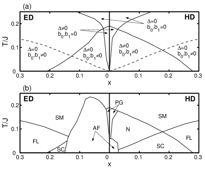
Figure 1: (a) Regions in the ($x$-$T$) plane where $\Delta=0$ or $\Delta\neq 0$ as well as $b_{0}=b_{1}=0$ or $b_{0},b_{1}\neq 0$. The dashed lines indicate the $T_{KT}$ described in the main text where long-range order in the dopon-spinon mixing channel is destroyed by vortex fluctuations. (b) The ($x$-$T$) phase diagram including the AF, SC, strange metal (SM), Fermi liquid (FL) and pseudogap with and without Nernst signal, labeled by N and PG respectively, regions. Both HD and ED cases are depicted in (a) and (b).

The MF phase diagram in Fig. 1a contains four MF phases, all of which are observed in the cuprates: (a) d-wave SC when $b_{0},b_{1},\Delta\neq 0$; (b) Fermi liquid when $b_{0},b_{1}\neq 0$ and $\Delta=0$; (c) pseudogap metal when $b_{0},b_{1}=0$ and $\Delta\neq 0$; (d) strange metal when $b_{0},b_{1},\Delta=0$.

We note that the MF SC transition temperature is very high in the underdoped regime. This is an artifact of the MF calculation since thermal fluctuations of the phases of the condensates $b_{0,1}$ are ignored. To crudely estimate the strength of $b_{0}$’s phase fluctuations, we note that the NN electron hopping term in $H_{tJ}$ induces a term $-\tfrac{|t_{1}|}{2}\chi\sum_{<ij>}(b_{0i}^{*}b_{0j}+h.c.)$. The resulting Kosterlitz-Thouless transition temperature T${}_{KT}=0.9|t_{1}|\chi b_{0}^{2}$, O9526 above which the condensate average $\bigl{<}b_{0}\bigr{>}$ vanishes due to phase fluctuations, is plotted as the dashed-line in Fig. 1a. The state with long-range SC order only appears below T_KT (see Fig. 1b). Above T_KT, and in the underdoped regime, there appear two distinct pseudogap metal regions marked by N and PG in Fig. 1b. In region N, which is located between the MF $T_{c}$ and T_KT, the non-vanishing magnitude of the MF order parameters $b_{0,1}$ leads to short-range SC correlations. This regime is observed experimentally, as suggested by the large Nernst signal measured in underdoped HD materials far above T_c. OW0409 ; US In the PG region $b_{0,1}=0$ and SC fluctuations become too small to be detected.

In the above MF calculation we have ignored the AF phase. To include this state we further introduce the MF decoupling channels $m=(-)^{i_{x}+i_{y}}\bigl{<}S_{i}^{z}\bigr{>}$ and $n=-\tfrac{(-)^{i_{x}+i_{y}}}{16}\bigl{<}\sum_{\nu=2,3}t_{\nu}\sum_{\hat{u}\in\nu\,NN}d_{i}^{\dagger}\sigma_{z}d_{i+\hat{u}}+h.c.\bigr{>}$ that account for the staggered magnetization in the lattice spin and dopon systems respectively. We thus add $2J^{*}Nm^{2}-4Nmn-2(J^{*}m-n)\sum_{\bm{k}}\psi_{\bm{k}+(\pi,\pi)}^{\dagger}\psi_{\bm{k}}-2m\sum_{\bm{k}}(\gamma_{\bm{k}}+\mu_{d})\eta_{\bm{k}+(\pi,\pi)}^{\dagger}\eta_{\bm{k}}$ to $H_{tJ}^{MF}$, where $J^{*}=\lambda\tilde{J}$ and $\lambda=0.31$ is a renormalization factor that enforces the transition between AF and SC orders at $x=0.03$ on the HD side. BL0202 Without addressing the issue of coexistence of AF and SC, we obtain the AF phase shown in Fig. 1b. The hopping parameters in the ED regime favor intrasublattice hopping processes which do not frustrate AF. TM9496 Also, on the ED side dopons are located around $(\pi,0)$, which is away from the nodal points, thus weakening SC in the ED regime (it is destroyed at lower doping than in the HD regime). Therefore, AF order is very robust on the ED side where it extends over most of the SC dome and where it covers the pseudogap region N (in conformity with the lack of a vortex induced Nernst signal on these materials BH0320 ).

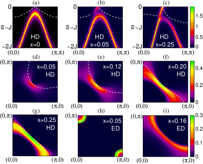
Figure 2: Electron spectral weights at $T=0$. (a)-(c) Evolution of the nodal direction electron spectral function with hole doping (top color scale). The white dashed line depicts the $\epsilon_{1,\bm{k}}^{-}$ band. (d)-(g) Electron spectral weight of the $\epsilon_{1,\bm{k}}^{-}$ band states for different $x$ in the HD regime (middle color scale). The white dashed line represents the minimum gap locus. The spectral weight at the node for $x=0.05,0.12,0.20,0.25$ is $0.21$, $0.35$, $0.45$ and $0.49$ respectively. (h)-(i) Integrated electron spectral weight for $x=0.05,0.16$ in the ED regime (bottom color scale). The energy window $[-0.15J,0.15J]$ was used. In (a)-(c) and (h)-(i) a Lorentzian broadening $\Sigma^{\prime\prime}(\omega)=-\tfrac{J}{10}$ was used.

To compare the above MF theory to ARPES we note that $c_{i,\sigma}=\widetilde{\mathcal{P}}\tfrac{1}{\sqrt{2}}(d_{i,-\sigma}^{\dagger}f_{i,\sigma}^{\dagger}f_{i,\sigma}f_{i,-\sigma}f_{i,-\sigma}^{\dagger}-d_{i,\sigma}^{\dagger}f_{i,-\sigma}^{\dagger}f_{i,\sigma})\widetilde{\mathcal{P}}$ is the electron annihilation operator and the electron creation operator in the HD and ED regimes respectively. Below, we ignore the incoherent contribution to the electron spectral function and use $c_{i,\sigma}=\tfrac{1}{\sqrt{2}}(d_{i,-\sigma}^{\dagger}+b_{0}f_{i,-\sigma}^{\dagger})$ instead. Figs. 2a-2c show how the MF electron spectral function along the nodal direction evolves with hole doping. These are self-consistent $T=0$ results concerning the SC phase. At $T=0$ only the two negative energy bands, namely $\epsilon_{1,\bm{k}}^{-}$ and $\epsilon_{2,\bm{k}}^{-}$, are occupied. For zero doping the spectral function contains only a peak at $\epsilon_{2,\bm{k}}^{-}$ (Fig. 2a). BROAD Upon doping spectral weight is transfered from the $\epsilon_{2,\bm{k}}^{-}$ to the $\epsilon_{1,\bm{k}}^{-}$ band, so that low energy quasiparticle weight develops above the parent insulator dispersion (hence inside the Mott gap!). As a result, in the underdoped regime two dispersive features arise. A linear dispersion crosses the Fermi level ($\omega\!\!=\!\!0)$ at a point that deviates from $(\tfrac{\pi}{2},\tfrac{\pi}{2})$ toward $(0,0)$. At higher energy, a band that resembles the dispersion of the undoped AF samples carries most of the spectral weight. Remarkably, this non-trivial behavior is also observed by ARPES KS0318 ; SR0402 and is to be contrasted with the conventional rigid band filling picture applicable to band insulators, namely that upon hole doping the chemical potential falls on top of the valence band forming hole pockets.

Notably, Figs. 2d-2g show that spectral weight transfered from the high energy to the low energy band distributes in momentum space in agreement with the nodal-antinodal dichotomy displayed by ARPES data: (a) The spectral weight associated with each state in the $\epsilon_{1,\bm{k}}^{-}$ band develops on an arc-shaped region around the nodal direction. KS0318 ; YZ0301 (b) In underdoped samples the spectral weight in the $\epsilon_{1,\bm{k}}^{-}$ band is depleted near the antinodal points and, as a result, the spectral structure in this $\boldsymbol{k}$-space region reflects only the high energy gap of $\epsilon_{2,\bm{k}}^{-}$ (which is reminiscent of the AF insulator). RS0301 (c) The total spectral weight in the $\epsilon_{1,\bm{k}}^{-}$ band increases with doping as the arcs extend to form a closed surface. (d) The coherence peaks in the antinodal region only appear around and beyond optimal doping. ZY0401 (e) A transition in the topology of the minimum gap locus from hole to electron-like at $x\approx 0.20$ is obtained. IK0204 ; BL0105 ; SL0402

Figs. 2h and 2i show that the MF low energy electron spectral weight distribution for the ED regime is also consistent with experiments. Indeed, at $x=0.05$ there is AF order and an electron pocket is formed around $(\pi,0)$ and $(0,\pi)$. AR0201 Further doping induces SC order and the d-wave SC quasiparticles develop spectral weight in the nodal region. As a result, a large “Fermi surface”, ungapped only along the nodal direction, is observed in Fig. 2(i). AR0201 ; CM0402

To conclude, in this letter we introduce a new, fully fermionic, MF approximation to the $tt^{\prime}t^{\prime\prime}J$ model. We also fit the MF parameters $t_{1,2,3}$ to ARPES data to argue that this MF approach is relevant to both HD and ED cuprates. As supported by the fact that $t_{1,2,3}\sim J$, the renormalization of the hopping parameters results from quantum spin fluctuations. Further work is required to properly understand the doping dependence of $t_{1,2,3}$, which reflects the change of spin correlations as the system is doped. Remarkably, though, the MF approach correctly accounts for the evolution of low energy spectral weight from the undoped to the overdoped regime only by fitting the $\epsilon_{2,\bm{k}}^{-}$ band to ARPES and by setting $t_{1}=2J$. ANISOTROPY We stress that fitting the renormalized parameters $t_{1,2,3}$ to ARPES also leads to a relatively quantitatively correct phase diagram.

We analyze ARPES lineshapes in the cuprates in terms of a two-band description of the interplay between spin and charge dynamics. Related two-band interpretations were also proposed by numerical studies. R0402 ; DZ0016 In Ref. DZ0016, quantum Monte-Carlo results for the large $U$ Hubbard model were interpreted in terms of two different states: (a) holes on top of an otherwise unperturbed spin background and (b) holes dressed by spin excitations. Similarly, in Ref. R0402, the nodal-antinodal dichotomy of the single hole $tt^{\prime}t^{\prime\prime}J$ model was understood in terms of two types of states where: (a) the vacancy is surrounded by a staggered spin pattern and (b) the vacancy is surrounded by spins that screen the hole spin-1/2 away. In this MF approach the doped carrier can also be surrounded by two different spin structures: (a) in the one-dopon state the vacancy is encircled by a local AF configuration of spins and (b) when the spinon and dopon mix the vacancy is encircled by a local spin singlet configuration. SCREEN In case (a) NN hopping is strongly frustrated (in our MF approximation it is actually set to zero). However, in case (b) quasiparticles coherently hop between different sublattices – this fact shows up in the linear quasiparticle dispersion across the Fermi point [near $(\tfrac{\pi}{2},\tfrac{\pi}{2})$] (Figs. 2b-2c). The kinetic energy gain that follows the emergence of NN hopping stabilizes the formation of spinon-dopon pairs which lead to the SC phase. It also prevents the collapse of the chemical potential on top of the AF insulator band, SR0402 thus explaining the lack of hole pockets, in accordance with experiments. KS0318 ; SR0402

References

(1) A. Damascelli et al., Rev. Mod. Phys. 75, 473 (2003).
(2) X.J. Zhou et al., Phys. Rev. Lett. 92, 187001 (2004).
(3) F. Ronning et al., Phys. Rev. B 67, 165101 (2003).
(4) Y. Kohsaka et al., J. Phys. Soc. Jpn. 72, 1018 (2003).
(5) A. Ino et al., Phys. Rev. B 65, 094504 (2002).
(6) T. Yoshida et al., Phys. Rev. Lett. 91, 027001 (2003).
(7) T. Tohyama et al., J. Phys. Soc. Jpn. 69, 9 (2000).
(8) W.-C. Lee et al., Phys. Rev. Lett. 91, 057001 (2003).
(9) T.C. Ribeiro, cond-mat/0409002.
(10) L. Krusin-Elbaum et al., Phys. Rev. Lett. 92, 097005 (2004).
L. Krusin-Elbaum et al., Phys. Rev. B 69, 220506(R) (2004).
(11) G.B. Martins et al., Phys. Rev. B 60, R3716 (1999).
(12) X.-G. Wen and P.A. Lee, Phys. Rev. Lett. 76, 503 (1996).
(13) C. Kane et al., Phys. Rev. B 39, 6880 (1989).
(14) W. Rantner and X.-G. Wen, Phys. Rev. B 66, 144501 (2002).
(15) K.M. Shen et al., Phys. Rev. Lett. 93, 267002 (2004).
(16) N.P. Armitage et al., Phys. Rev. Lett. 88, 257001 (2002).
(17) A. Lanzara et al., Nature 412, 510 (2001).
(18) and reflect the local and non-local mixing of
spinons and dopons.
If the term in
drives local mixing. If the term
in leads to non-local mixing.
Hence, either are both zero or both non-zero.
(19) P. Olsson, Phys. Rev. B 52, 4526 (1995).
(20) N.P. Ong et al., Annalen der Physik 13, 9 (2004).
(21) I. Ussishkin et al., Phys. Rev. Lett. 89, 287001 (2002);
I. Ussishkin and S.L. Sondhi, cond-mat/0406347 (2004).
(22) J. Brinckmann and P.A. Lee, Phys. Rev. B 65, 014502 (2002).
(23) T. Tohyama and S. Maekawa, Phys. Rev. B 49, 3596 (1994).
(24) H. Balci et al., Phys. Rev. B 68, 054520 (2003).
(25)
The sharp MF peak in the high energy
band is broadened by fluctuations around MF level.
(26) P.V. Bogdanov et al., Phys. Rev. B 64, 180505(R) (2001).
(27) C.T. Shih et al., Phys. Rev. Lett. 92, 227002 (2004).
(28) T. Claesson et al., Phys. Rev. Lett. 93, 136402 (2004).
(29) For instance, as the high energy pseudogap closes
upon doping, the band approaches the
band around and leads to the increase of
low energy spectral weight in the antinodal region seen in experiments.
(30) A. Dorneich et al., Phys. Rev. B 61, 12816 (2000);
C. Gröber et al., Phys. Rev. B 62, 4336 (2000).
(31) Upon spinon-dopon mixing the term
becomes . It then describes the decay of the dopon into
a spinless spinon-dopon pair and a chargeless spinon.
Physically, this process means that the vacancy is encircled by a local
spin singlet configuration while the doped carrier spin-1/2 is
taken away by the spin background.