A Statistical Mechanical Load Balancer for the Web

Abstract

The maximum entropy principle from statistical mechanics states that a closed system attains an equilibrium distribution that maximizes its entropy. We first show that for graphs with fixed number of edges one can define a stochastic edge dynamic that can serve as an effective thermalization scheme, and hence, the underlying graphs are expected to attain their maximum-entropy states, which turn out to be Erdös-Rényi (ER) random graphs. We next show that (i) a rate-equation based analysis of node degree distribution does indeed confirm the maximum-entropy principle, and (ii) the edge dynamic can be effectively implemented using short random walks on the underlying graphs, leading to a local algorithm for the generation of ER random graphs. The resulting statistical mechanical system can be adapted to provide a distributed and local (i.e., without any centralized monitoring) mechanism for load balancing, which can have a significant impact in increasing the efficiency and utilization of both the Internet (e.g., efficient web mirroring), and large-scale computing infrastructure (e.g., cluster and grid computing).

I Introduction and Motivation

In the past several years there has been significant progress in the field of complex networks due to an infusion of ideas from statistical mechanics. Some of the branches of statistical mechanics that have informed the study of complex networks include percolation theory Newman and Watts (1999a); Moore and Newman (2000); Callaway et al. (2000); Dorogovtsev et al. (2001), renormalization group methods Newman and Watts (1999b), Bose-Einstein condensation Albert and Barabasi (2002); Bianconi and Barab si (2001) and partition function methods for the study of equilibrium uncorrelated Dorogovtsev et al. (2003a); Burda and Krzywicki (2003); Burda et al. (2001) and correlated Berg and Lassig (2002) random networks.

These analytical tools have led to the formulation of a number of protocols or stochastic dynamics for complex networks that result in predictable macroscopic properties. For example, preferential attachment based dynamics, provide both models for how existing networks might have evolved Newman and Park (2003); Jin et al. (2001); Handcock and Jones (2003); Lehmann et al. , as well as how one might engineer ad hoc systems such that the resulting networks have desired global properties such as power-law degree distributions and tolerance to both attacks and failures Sarshar and Roychowdhury (2004); Albert et al. (2000). Dynamics on such networks, such as percolation and random walks, have led to efficient algorithms for searching in PL random networks and peer-to-peer systemsSarshar et al. (2004).

In this paper, we build on such studies and introduce a network dynamical system such that the steady state degree distribution will be tightly clustered around the average value. The well known ER graphs have such a tight clustering property: the probability of deviating from the mean decreases exponentially with the deviation distance. In order to design such a dynamical system, we model it after a physical system with say a fixed energy, and make use of the maximum entropy principle. That is, we introduce an edge dynamic for networks with fixed average number of edges and fixed number of nodes, and show that the dynamic can never decrease the entropy of the system. Thus, our edge dynamic can be viewed as an effective thermalization process, and the fixed average number of edges can be considered to be a physical system with constant energy in a statistical mechanical sense. The maximum-entropy degree distribution for a network with fixed number of edges corresponds to that of ER random graphs with a binomial distribution. Thus, the maximum entropy principle dictates that the network system would tend towards an ER random graph.

We provide further analytical results, based on a rate-equation approach, which show that the steady state distributions do indeed correspond to ER graphs. We also show how local protocols using short random walks can effectively emulate the original global edge dynamics, thus providing a local and distributed stochastic algorithm for a network to self-organize itself into ER random graphs. We provide extensive simulations of our local dynamics and show that the convergence to ER random graphs is robust even if the protocols are modified in different ways to suit practical implementation requirements.

We find that the dynamical system studied here can provide an effective load balancing paradigm for the distributed resources accessible on the Internet. As the popularity of the Internet has increased, so too has the need for highly scalable web server software. Every major web site uses mirrors to, among other things, balance the request load over multiple servers. This service is currently provided by companies such as Akamai which maintain proprietary overlay networks with tens of thousands of nodes and which routinely handle double-digit percentages of total Internet traffic. An overlay network is simply a virtual network built on top of an existing network. Overlay networks often add new features not found in the underlying network or make certain operations more convenient. The most famous example of an overlay network is the Internet. The Internet consists of computers and routers which are connected by different physical links (ethernet, ATM, phone-line, wireless ,etc.), however the Internet Protocol creates a virtual IP network that allows the networked computers to be addressed without knowledge of the physical transport layer; providing a higher level of abstraction is often a goal of overlay networks. The overlay network that we propose can be built directly on of any of the physical transport layers mentioned above or it can use the Internet as the underlying network. Thus an overlay network need not consist of physical links between nodes. In an addressable network such as the Internet, the edges may simply be a table of addresses that each node maintains to represent its neighbors in the overlay. Of course in networks that are not globally addressable, the overlay edges will be actual open links that are continuously maintained over the physical network or alternatively each node can maintain a routing table that gives complete route information on how to reach its neighbors.

A system using the techniques proposed here can provide effective load balancing for Open Source software projects and other organizations seeking non-commercial mirroring solutions. Good examples of such projects include the Linux kernellin and Debian GNU/Linux deb . Each project has hundreds of mirrors that are chosen arbitrarily by users and thus the demand variance of the mirrors can be quite large. On the other hand, if each of the mirrors can automatically redirect traffic to less loaded mirrors the users would have a more reliable service, and the servers would have a more predictable load.

To state the problem as simply as possible, we consider a system of $N$ comparable-capacity web servers all of which mirror the same set of contents. For efficient usage of these resources, one would want to distribute the download requests as evenly as possible, so that no server is significantly more loaded than others. The question is, can one achieve such a load balancing task, without a centralized server or some equivalent mechanism to monitor the global state of the network. Numerous load-balancing applications for web servers Wolf and Yu (2001); Cardellini et al. (2002); Andreolini et al. (2002) based on global monitoring have been proposed and several open source projects have formed to provide capacity and geography load-balancing sup ; ult ; lvs .

We present a scheme fundamentally different from those proposed in the literature: instead of monitoring servers and their availability via a static network, we create a dynamic overlay network that provides both a measure of instantaneous load distribution, and dynamics for job allocation and resource update. The way we adapt our dynamical network system to the task of load balancing is as follows. First, a node’s in-degree is made to correspond to the unused capacity or instantaneous estimate of the free resources of a node. Second, the edge dynamics in our system are used to perform the job allocation and resource updating tasks for the load balancing process. That is, when a new job arrives the node receiving the job chooses, via a random walk (as prescribed by our edge insertion dynamic), the node which is going to execute the job. The target node on receiving the job removes one of its incoming edges to reflect the reduced availability of its resources. Similarly, when a node/server completes a job, then to reflect its state of being more ready to receive a job, it adds an incoming edge to itself (again via a random walk, as prescribed by our edge insertion dynamic) to increase its in-degree. In steady state, the rate at which jobs arrive would equal the rate at which jobs are completed, and hence the underlying network has a fixed average number of edges.

Thus, a dynamic overlay network, connecting all the servers, emerges. The state of this network (in particular, as indexed by the in-degree distribution of the nodes) represents the instantaneous distribution of load over all the servers. The job assignment and the resource update steps, performed according to the edge deletion and insertion steps in our network dynamics, guarantees that the distribution of load will be fair across all the servers in the network: the underlying graph will be close to an ER random graph with a binomial degree distribution.

We have made several simplifying assumptions here so as to show a proof of concept for this scheme. For example, we are implicitly assuming that the servers have comparable capacities and that any job can be assigned to any of the servers. A complete treatment of how to adapt our approach to address these practical issues, is beyond the scope of this paper, and will be treated in future work. We provide general guidelines how our scheme can be generalized in the discussion section of the paper. Nevertheless, the scheme proposed here can be implemented as it is, without any major modifications, and increase the efficiency and utilization of tasks such as web mirroring on the Internet.

This paper has the following structure. Section II describes our network dynamical system and shows why we should expect it to lead to an ER random graph from the perspective of the maximum entropy principle. Section III gives a steady state solution for the degree distribution of the nodes and thus provides an analytical argument as to why the system will converge to ER random graphs. In section IV, we show how the dynamics can be simulated via random walks on the underlying graphs and with as little global information as possible. We also present extensive simulation results demonstrating the robustness of the system. Finally in section V, we discuss how a load-balancing problem can be efficiently mapped to our statistical mechanical system and present more simulation results to show the efficacy of our approach.

II Maximum Entropy Principle

It is well known that for a fixed expected number of edges, the maximum entropy graph is the ER graph with a binomial degree distribution. We can see this by the method of Lagrange multipliers. Suppose $p_{i}$ is the probability that a node has $i$ incoming edges. The expected number of edges in the graph is $E=N\sum ip_{i}$. Putting into place a constraint on the expected number of edges and the normalization of $p_{i}$, we get the following Lagrangian:

$$\mathcal{L} = -N\sum_{i}p_{i}\log p_{i}$$

$$\mbox{+}N\sum_{i}p_{i}\log{N-1\choose i}$$

$$\mbox{}+\alpha N\sum_{i}ip_{i}+\beta N\sum_{i}p_{i}$$

$$\frac{1}{N}\frac{\partial\mathcal{L}}{\partial p_{i}} = -(1+\log p_{i})+\log{N-1\choose i}$$

$$\mbox{}+\alpha i+\beta$$

Setting $\frac{\partial\mathcal{L}}{\partial p_{i}}=0$, and using the fact that $\sum_{i}p_{i}=1$ and $\sum_{i}ip_{i}=E/N$, we get:

$$p_{i} = {N-1\choose i}q^{i}(1-q)^{N-1-i}$$ (1)

$$q = \frac{E}{N(N-1)}$$

Recall that an equivalent description of a directed ER graph is as follows: for each node there are $(N-1)$ possible incoming edges, each of which is selected independently and with probability $q$ (as defined above).

Next we consider a directed graph with $N$ nodes and $E$ edges. At each step, a randomly selected existing edge is deleted. Additionally, a randomly selected absent edge is inserted. This dynamical system then can be considered as a statistical mechanical system, and we may ask if the edge dynamic is an effective thermalizing scheme or not; that means, we have to show that the entropy of the system after every step never decreases.

We use standard information theoryCover and Thomas (1991) notations for entropy:

$$H(G)=-\sum_{g}Prob(G=g)\log Prob(G=g)\ .$$

The entropy of a graph is exactly the average number of bits it requires to describe its configuration, or equivalently, the $\log$ of the number of states it is likely to occupy. Consider the example of an ER random graph, $G_{ER}$, with $E$ directed edges present of $E_{m}=N(N-1)$ possible edges and $N=|V|$ nodes. There are $|G_{ER}|$ such graphs and each is equally likely since each possible edge exists in the graph with the same probability.

$$|G_{ER}|={E_{m}\choose E}$$ (2)

Thus the entropy of an ER graph is:

$$H(G_{ER}) = -\sum_{g\in G_{ER}}\frac{1}{|G_{ER}|}log\frac{1}{|G_{ER}|},$$ (3)

$$= log|G_{ER}|$$

However it will not be necessary to compute $H(G)$ directly since we will only be concerned with the change in entropy when random edges are inserted and deleted.

Using $H(G)$ as the entropy of the graph $G$, we can see that after each time step, the entropy of the graph has increased, such that:

$$H(G_{i+1}) \geq H(G_{i})$$

The proof is the following. Define, $B$ as the graph before a given time step, and $A$ as the graph after a given time step. Using the notation $p(a)=Prob(A=a)$ The conditional entropy $H(A|B)$ is given from the conditional probability distribution:

$$H(A|B) = \sum_{b}p(b)H(A|B=b)$$

$$= -\sum_{b}p(b)\sum_{a}p(a|b)\log p(a|b)$$

$$= -\sum_{a,b}p(a,b)\log p(a|b)$$

Using the mutual informationCover and Thomas (1991) $I(A;B)$ we obtain:

$$I(A;B) = H(A)-H(A|B)$$

$$= H(B)-H(B|A)$$

$$H(A)-H(B) = H(A|B)-H(B|A)\ .$$

Since $Prob(A=a|B=b)$ is given by the update rule, where $a$ is the graph after an update, and $b$ is the graph before an update, $H(A|B)$ can be computed from the graph update rule. There are $E_{m}$ maximum edges in the graph, and $E$ edges at a given time. In a directed graph $E_{m}=N(N-1)$. The entropy of our random edge selection is $\log E$ which is the $log$ of the number of edges from which the random selection is made. We add an edge by selecting a random edge to add, from all the edges that are not there. The change in entropy of this operation is $\log(E_{m}-(E-1))$ which is the $log$ of the number of absent edges. Thus:

$$H(A|B) = \log E+\log(E_{m}-(E-1))$$

Computing $H(B|A)$ will in general depend on the prior distribution $P(B)$, however we know that the prior can only reduce entropy from the maximum. We don’t know which edge was just added to $A$, but no matter what $P(B)$ is, an upper bound on the entropy is the uniform assumption: giving entropy $\log E$. Likewise, if we know $P(B)$, we can find a probability distribution on which edge was the edge which was deleted to arrive at $A$, however, the most the entropy can be is $\log(E_{m}-(E-1))$, thus:

$$H(B|A) \leq \log E+\log(E_{m}-(E-1))$$

Which gives us the principle that entropy is never decreasing:

$$\Delta H = H(A)-H(B)$$

$$= H(A|B)-H(B|A)$$

$$= \log E+\log(E_{m}-(E-1))-H(B|A)$$

$$\geq 0$$

So, entropy can never decrease. If the number of edges in a graph is fixed, the maximum entropy distribution means that all graphs with that fixed number of edges are equally likely. If we have a large ER graph with $p=E/(N(N-1))$, we expect there to be $E$ edges. The Chernoff bound tells us that the probability that an ER graph has more or less than $E$ edges falls exponentially. Thus, we expect the system to tend towards an ER random graph. The binomial distribution means that each node will have a degree which is close to the mean degree and that nodes with degree much higher or much lower than average are rare.

Dorogovtsev et. al. Dorogovtsev et al. (2003b) discuss a similar dynamical model, where the total number of edges is fixed and an edge rewiring scheme is introduced. However, the analysis is done with a view towards the production of power-law graphs and arbitrary fat-tailed distributions.

The model presented in this section can be modified to one where only the expected number of edges is constant, however the algebra will become more complex. As shown analytically in Section III and via simulations in Section IV, we can relax the constraint that the number of edges be fixed, make the numbers deleted and inserted random variables, and the result will remain an ER graph.

III Rate-Equations for the In-Degree Distribution

In this section we provide a rate-equation based analysis of the in-degree distribution of nodes in a stochastic network system similar to the one introduced in section II. While the entropy analysis considered graphs that lose and gain exactly one edge each time step, in the rate equation approach the number of edges created and destroyed are both random variables that are chosen to produce a constant average in-degree. In particular, let us consider the dynamics from the perspective of the nodes. For reasons that will be apparent in the section on load balancing, we will denote the average number of absent edges in the graph as $J$, and assign an integer $C$ as the maximum in-degree of any node; $C=N-1$ corresponds to the case considered in the previous section. Thus, the average number of edges (which is the same as the sum of the in-degrees of all the nodes) in the network is $E=NC-J$.

Let a randomly picked node have in-degree $i$ during a certain step. Each edge is deleted uniformly and independently, thus the probability that a node with $i$ incoming edges will lose at least one edge is approximately proportional to its in-degree. Note that the expected number edges deleted per step in the whole network is $1$, and hence, we can ignore the case where more than one incoming edge is deleted at the same node. Hence, the rate at which the node’s degree will decrease by one can be approximated as:

$$\mu_{i}=\begin{cases}\frac{i}{NC-J}&\text{$(0\leq i\leq C)$}\cr 0&\text{else}\cr\end{cases}$$ (4)

Similarly, the rate at which it will acquire an edge (i.e., its degree will increase by one) can be assumed to be proportional to $(C-i)$ (i.e., the number of possible incoming edges that are absent):

$$\lambda_{i}=\begin{cases}\frac{C-i}{J}&\text{($0\leq i\leq C$)}\cr 0&\text{else}.\cr\end{cases}$$ (5)

The above process then can be seen as a birth and death Markovian process with state-dependent arrival and service(departure) rates. Markov processes like this often appear in queueing theory and in that context this is an M/M/$\infty$//M queueing systemKleinrock (1975).

In our situation, the states of the Markov process correspond to the instantaneous in-degree of a node (hence, the total number of states is $C+1$), and the rates at which its degree decreases and increases are given by Equs. (4), and (5), respectively. If the probability of being in state $n$ (i.e., the probability that a randomly picked node has degree $n$) is $p_{n}$, then the steady state distribution satisfies the following:

$$B = \{j:1\leq j<C\},$$

$$0 = -(\lambda_{j}+\mu_{j})p_{j}+\lambda_{j-1}p_{j-1}+\mu_{j+1}p_{j+1}$$

$$\qquad(\forall j\in B).$$

Which we rewrite as:

$$(\mu_{j+1}p_{j+1}-\lambda_{j}p_{j})=(\mu_{j}p_{j}-\lambda_{j-1}p_{j-1}).$$ (6)

The boundary condition is:

$$0 = -\lambda_{0}p_{0}+\mu_{1}p_{1}.$$

By solving equation 6 we obtain a simple steady-state solution for the expected distribution of jobs per node. To solve this difference equation define $\alpha_{j+1}=\mu_{j+1}p_{j+1}-\lambda_{j}p_{j}$, and note the equation becomes:

$$\alpha_{j+1} = \alpha_{j}$$

$$0 = \alpha_{0}$$

Thus, $\alpha_{j}=0$, or equivalently:

$$p_{j+1} = \frac{\lambda_{j}}{\mu_{j+1}}p_{j}.$$

The solution of the above is:

$$p_{n} = p_{0}\prod_{i=0}^{n-1}\frac{\lambda_{i}}{\mu_{i+1}},$$ (7)

$$= p_{0}\frac{C(C-1)(C-2)\cdots(C-n+1)J^{-n}}{n!(NC-J)^{-n}},$$

$$= p_{0}\left(\frac{NC-J}{J}\right)^{n}{C\choose n}.$$

We know that $\sum_{n}p_{n}=1$, and thus we see that $p_{n}$ is binomially distributed:

$$p_{n} = {C\choose n}\left(1-\frac{J}{NC}\right)^{n}\left(\frac{J}{NC}\right)^{C-n}.$$

If we define a normalized quantity as $\alpha=J/NC$ ($\alpha$ will have a physical meaning in the context of the load balancing system discussed in section V ), then we get the variance of the distribution to be $\sigma^{2}=C\alpha(1-\alpha)$.

If $C=N-1$, then we see that this model recovers the ER graph we found in Section II:

$$p_{n} = {N-1\choose n}q^{n}(1-q)^{N-1-n}.$$

Where $q=\frac{E}{N(N-1)}$ and $E=N(N-1)-J$.

IV Local Dynamics and Simulation Results

Implementing the exact graph dynamics discussed in the two previous sections would require global knowledge about individual node’s degrees and/or the number of edges in the network at any step. However, it would be ideal to be able to have a stochastic dynamic that just samples the graph using local information, and makes decisions about which edges to add or delete. Eq. (4) provides a useful lead: it implies that a node loses an edge preferentially with respect to its in-degree. We know that if one performs a long-enough random walk on an undirected graph (or a Eulerian directed graph) then in steady state the probability that the walk will end at a particular node is proportional to its in-degreeLovász and Winkler (1995). The issue is about the required length of the random walk. Ideally we would like to do a walk of length no more than $O(\log N)$; we justify in the following remarks why a logarithmic length random walk suffices for our case and also provide simulation evidence.

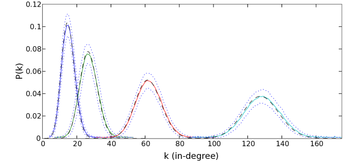
Figure 1: The proposed edge dynamic generates Erdös-Rényi random graphs. The steady state in-degree distributions are shown for the random-walk based network dynamics described in section IV. These graphs have $N=1024$, maximum in-degree $N-1$, and average in-degrees (from left to right) of $16$, $32$, $64$ and $128$ respectively. Each graph begins as a completely structured graph with $O(N)$ diameter. After the edge dynamics thermalizes the graph, the result is an Erdös-Rényi random graph with $O(\log{N})$ diameter. The mean distributions (solid lines) are each shown with upper and lower standard deviation range curves (dotted lines). The predicted binomial degree distributions (dashed lines) are shown for comparison. Arrivals and departures at each time step are Poisson distributed.

In order to verify that local dynamics do indeed lead to ER graphs and match the theoretical predictions, we performed extensive simulations with several protocols and the results are reported in this and the following sections. We intentionally introduced certain deviations from the exact protocol discussed in sections II and III so as to demonstrate the robustness of the whole system and keep the protocols relevant for load balancing systems studied in this paper.

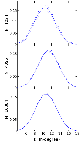
Figure 2: The production of Erdös-Rényi random graphs using the random-walk based dynamics discussed in section IV is effective for all network sizes simulated (at least up to $N=16384$). These in-degree distributions (solid lines) are for graphs with $N=1024$, $N=4096$ and $N=16384$. Standard deviation range curves are shown as dotted lines. These graphs have an imposed maximum degree, $C=22$, and a mean in-degree of approximately $11$. With increasing $N$ we see tighter convergence to the binomial distribution. Arrivals and departures at each time step are Poisson distributed.

1. Graph Initialization: First we create a directed graph with $N$ nodes and $E=N\langle k\rangle$ edges such that the maximum degree of any node is $\leq C$ (note the case of no restrictions on the maximum degree, i.e., $C=N-1$, is considered in Figs. 1 where as the case of restricted maximum degree is considered in Figs. 2 and 3 ). This graph is intentionally constructed in a very structured fashion so as to show that the proposed dynamics do indeed lead to a random graph independent of the initial configuration. The initial structure is created by connecting node $i$ by incoming edges to nodes $(i+1)\mod N$, $(i+2)\mod N$, $\cdots$, and $(i+\langle k\rangle)\mod N$, where $\langle k\rangle$ is the average degree of the nodes. Further evidence that the dynamics effectively randomize the initial graph can be seen from the fact that the initial graphs have a diameter of $O(N/\langle k\rangle)$ while the thermalized graphs have diameter bounded above by $O(\log N)$.

2.Edge deletion: For this set of simulations, at each time step we delete a Poisson-distributed number of edges. A random walk of length $\log N$ (i.e., of lengths 10 ,12 and 14 in the simulations reported in Figs. 2 ) is initiated from a fixed particular node, and the last node on the random walk randomly deletes one of its incoming edges.

3. Edge Insertion: Ideally, we should insert an edge picked randomly among the absent edges. One way to achieve this would be to do a random walk on the complementary graph $\bar{G}$ (i.e., where the absent edges in $G$ are present) and pick the node it ends at as the arrow-end of the edge to be inserted; i.e., the node, $i$, the random walk ends at gets an incoming edge. To decide on the node that will get the outgoing edge, one could reverse the directions of the edges in the complementary graph $\bar{G}$, and perform a random walk starting at the node $i$ (found in the previous step), and select the node, $j$, that the random walk ends at. Then a directed edge from node $j$ to node $i$ is added. The two steps ensure that both the in-degree and the out-degree of a node increase proportional to its respective absent degree (i.e., the number of all possible edges that are missing; see Eq. (5)).

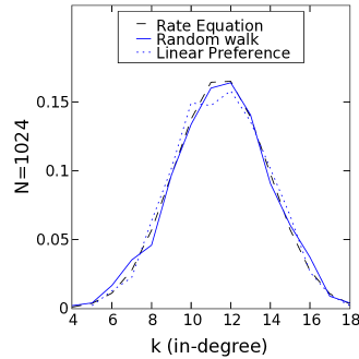
Figure 3: The simulated networks generated by short random walk dynamics with a fixed number of edges are very similar to networks produced by global linear preferential selection dynamics. The random walk job migration (solid line) and the global preferential job allocation (dotted line) described in section III Eq.(4) produce in-degree distributions that match well to the predicted binomial distribution. The random walk simulation graph has a constant number of edges and is thus very similar to the rewiring dynamic described in section II . The linear preference simulation uses global linear preference to distribute jobs rather than the local random walk approximation. Along with Fig.4 this shows that random walks can be used to approximate linear preferential selection of nodes. Single snapshots of the distributions are depicted rather than distribution averages shown in Figs. 1, 2 and 5. Table 1 summarizes the simulation parameters and distribution variances.

In our protocol, however, we take into consideration the fact that a random walk on the complementary graph is not needed or feasible in certain applications. Moreover, in the load-balancing application considered in the next section the absent edges of the graph correspond to jobs that are occupying the resources of the node. Therefore, the addition of an edge is undertaken when a node finishes one of its jobs and wants to increase its in-degree. Thus, in one simulation reported in Fig.3 and Table 1, we assume that a node is chosen randomly proportional to its missing degree to receive an incoming edge. Since missing degrees are proportional to the number of jobs on a node, the above assumption is equivalent to assuming that each job ends with equal probability at each time step (or that job length follows a geometric distribution). This decision is made globally; the situation where each node independently makes its decision to accept an incoming edge (thus following Eq. (5) exactly) based on the detailed simulated execution of resource-consuming jobs on resource-bearing nodes will be reported in future work. Now in order to find the other end of the edge, instead of performing a random walk on the complementary graph (with edges reversed), we still perform a random walk on the graph $G$ starting at the node selected to receive an incoming edge, and select the node that the random walk ends at. This has the consequence that the out-degree distribution will deviate somewhat from the ER prediction (see Fig.5). For the purpose of the proposed load balancing system this is not a liability since the out-degree of a node is not physically meaningful.

Here are a few additional remarks about the graphs generated and our simulation results and local random-walk based protocols:

1. Minimum Degree of a node: The connectivity and diameter of random graphs are both well-established and are critical measures of performance. For instance, in order for a random graph to have a giant component, the average degree, $\langle k\rangle$, must be greater than 2. If $\langle k\rangle>7/2$, then the diameter of a random graph scales logarithmicallyAlbert and Barabasi (2002):

$$d(k,N)\propto\frac{\ln N}{\ln\langle k\rangle}$$ (8)

These results apply to undirected random graphs and since we are focused on directed graphs we provide supporting simulation results to show that this protocol produces connected, strongly-connected and fast mixing directed graphs with low directed diameter.

If the network does not have a giant component, then many nodes will be isolated and unable to participate in a local search algorithm. The implications for load balancing applications will be discussed in section IV.

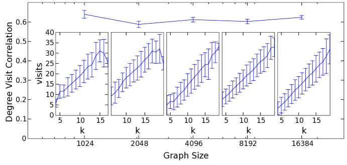
Figure 4: Short random walks are a good approximation to linear preferential selection. In Fig. 3 we observed that random walk dynamics and linear preferential selection produced similar degree distributions. Here we show directly that each node’s in-degree, $k$, is correlated to the frequency that random walks terminate at that node; we also demonstrate that this relationship holds for a range of network sizes. The correlation coefficient averaged over 100 snapshots of the graph is shown (solid line) at the top of the plot with standard deviation range bars. The consistent average correlation indicates that the approximate linear preference observed for short random walks scales over a range of networks sizes that exceeds an order of magnitude($N=1024$ to $N=16384$). The insets show that nodes have a number of visits linearly proportional to $k$ . In each inset the mean number of visits (solid line) and standard deviation range bars are plotted vs. node in-degree. Except for the minor deviations seen for $N=1024$ and $N=2048$, we see that short random walks produce a very close approximation to linear preference. In all cases the length of each random walk is $\log N$.

Ideally we want the graph to have no disconnected components and be strongly-connected; this will ensure that our random walk approach can properly thermalize the graph. Strictly speaking, we do not need the graph to have a single strongly-connected component at every step since the introduction of new edges should repair the graph and make it a single strongly-connected component often enough. The repairs can happen because the direction of an edge only affects the propagation direction for the random walks. An example of a connected (but not strongly-connected) graph is a pair of strongly-connected clusters, $A$ and $B$, with a single edge $e_{AB}$ going from a node in $A$ to a node in $B$. Random walks initiated in $B$ will never reach nodes in $A$ unless an edge from $B$ to $A$ is created. But such edges can be easily formed. When a node in $A$ needs a new incoming edge it initiates a walk to find a node to be the other side of the edge. When such a walk crosses $e_{AB}$ and ends at a node in $B$, a new edge $e_{BA}$ will be created that goes from $B$ to $A$.

In our simulations we do indeed find that strongly-connected components split and merge as the graph evolves. However in all simulations conducted with an imposed minimum degree of $4$ we observe that the network never permanently fragments into multiple strongly-connected components. Fluctuations occur but the graphs heal themselves. Although this does not constitute a proof that the graphs will always remain strongly-connected, we observe in all simulations that the number of strongly-connected components remains near $1$. This is an important practical concern for an implementation and more detailed simulation and analysis will be the subject of future work.

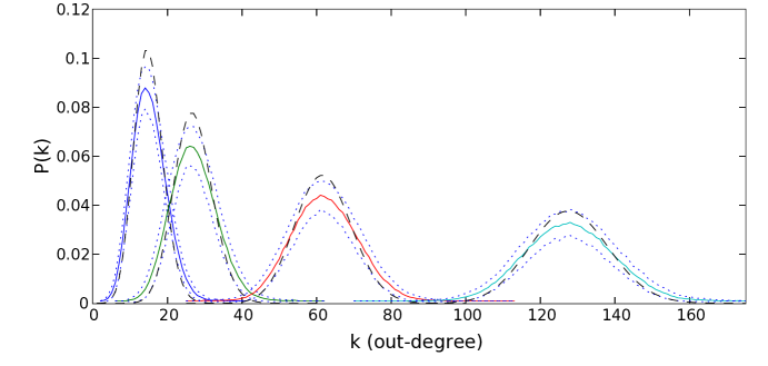
Figure 5: We see that these simulated graphs have out-degree distributions that deviate slightly from the binomial degree distributions. These out-degree distributions are from the same simulations presented in Fig.1. These graphs have $N=1024$, maximum in-degree $N-1$, and average in-degrees (from left to right) of $16$, $32$, $64$ and $128$ respectively. The out-degree distributions have similar averages but larger variances than the in-degree distributions. The mean out-degree distributions (solid lines) are each shown with upper and lower standard deviation range curves (dotted lines). Given that the in-degrees and out-degrees are subject to different dynamics we would not expect the out-degree distribution to follow the binomial distribution. Arrivals and departures at each time step are Poisson distributed.

2. Mixing time and the length of the Random Walks: It is known that for a random $d$-regular undirected graph, the mixing time (i.e., the length of the random walk necessary to sample edges uniformly, or equivalently, nodes preferentially) scales as $O(\log N)$, where $N$ is the number of nodes in the networkKahale (1995). It is widely believed that since an ER graph is almost a $\langle k\rangle$-regular graph, where $\langle k\rangle$ is the average degree of the nodes, the mixing time should also scale as $O(\log N)$. If the average degree is $\log N$, then one can prove this result; however, a formal proof is not there for ER graphs with constant average degree. For our case, however, $\log N$ average degree is quite reasonable; if $N=1048=2^{10}$ then the average degree has to be $10$ for the formal results to hold.

A related quantity to mixing time is the graph diameter. In order to sample edges uniformly using a $O(\log N)$ random walk the diameter of the graph cannot be larger than $O(\log N)$ since the walk must be able to reach every edge to sample uniformly. Starting with a structured graph with $O(N)$ diameter the thermalized graph that results from a few thousand iterations now has a diameter that is of $O(\log N)$ in all simulations conducted.

In order to verify that the random walks do indeed sample the nodes proportionally to their in-degree in these directed networks, we provide the following simulation results. After the evolving graph structure has stabilized we freeze the graph and select a node that initiates $20N$ random walks of length $(\log N)$. We record the number of times that each node is the last visited on a walk and then calculate the correlation between each node’s visitation frequency and in-degree. Figure 4 shows a high correlation coefficient. Also note that each node is visited at least once in all simulations which confirm the low diameter of the graph. Each node in the starting graph was selected to initiate the walks to show that the mixing is uniform throughout the graph.

3. Out-Degree Distributions: Although the in-degree distribution is of primary interest in this paper, we also briefly report the out-degree distribution here. In Figure 5 we see that the out-degree distribution does not match the ER distribution as closely as the in-degree. This lack of symmetry is due to the fact that the random walks performed when adding and removing edges travel over directed connections. If we wished the out-degree distribution to follow an ER degree distribution as closely as the in-degree we could follow a similar protocol for both for both in-degree and out-degree. However in this protocol the out-degree is not of interest and will not be considered in detail..

System type	$\sigma_{free}^{2}$
Rate equation prediction	5.49
Linear preference simulation	5.59
Random walk simulation	5.81

Table 1: Variances for random walk and linear preference simulations shown in Fig. 3 as well as the Binomial distribution maximum degree $22$, $1024$ nodes, and $10752$ jobs.

V A Load-Balancing Paradigm

V.1 Previous work

The field of load-balancing has been active for decades and many techniques and problem formulations have been used to approach the problem Lling et al. (1991); Casavant and Kuhl (1988); Peixoto (1996); Mitzenmacher (2001). The use of random walks has produced some interesting empirical load balancing results in sensor networks Avin and Brito (2004). What distinguishes the proposed protocol from prior work is the use of random walk sampling on an overlay network whose topology is actively shaped by the dynamics of the protocol. No monitoring is performed in this scheme since the load balancing algorithm and state information is encoded in the overlay network structure. Please note that this overlay graph need not consist of physical links as long as the network is globally addressable. Since the Internet is addressable, each node in an Internet-based overlay will only need to maintain a table of of its neighbor nodes rather than a physical connection for each neighbor. On the other hand in networks that are not globally addressable the overlay edges will need to contain complete route information or the edges will need to be actual physical links.

V.2 Statistical Mechanical Load-Balancer

Let us take the same statistical mechanical system as in the preceding sections and encode it as follows:
(i) Each node represents a server or processor providing service to a networked community.
(ii) The in-degree of a node represents the amount of free resources of the particular node, e.g., the number of extra jobs in can handle.
(iii) The maximum in-degree, $C$, is the maximum capacity that each node in the network can handle.
(iv) The state of the network, i.e., the in-degree distribution, represents how balanced the load distribution is.

In the steady state, jobs/requests arrive at the same rate as the jobs are completed by the suite of servers. Hence, when a job arrives (by random walk), in order to represent the node’s increased load and decreased free resources, we may need to decrease the in-degree of the node that received the new job; this is done by deleting one of its incoming edges uniformly randomly. Similarly, when a job completes, the corresponding server may have excess free resources and it should indicate its new state by increasing its in-degree; this is done by performing a short random walk and making a new directed edge that originates at the last node on the random walk and terminates at the node that initiated the walk.

The outline of the steps is summarized below.

• Create a graph $G$ whose nodes have in-degree proportional to free resources.

• When a node, $v_{i}$, creates new load, it performs a short random-walk on $G$ and distributes the new load to the end node on the walk.

• Nodes compensate for changes in load by creating or deleting edges in accordance with the prescribed edge dynamic which keeps the in-degree of a node proportional to its free resources. Newly arrived jobs can delete edges while jobs that are completing can create new edges.

The dynamics we have proposed in the previous section create and maintain the structure of the overlay network through the deletion and creation of edges. This resulting overlay network is an ER graph (or its variant studied in section III that has a bounded number of in-degrees $C$) which is an almost regular graph.

Mapping the properties of this overlay network to node resources can be handled easily by making the natural assumption that there is a scalar metric, $R$, that each node can locally calculate to determine its free resources. For web mirroring the relevant metric is the bandwidth that the next request can expect to receive. It would be calculated as the peak outgoing bandwidth $B_{i}^{(max)}$ divided by the current number of requests $D_{i}$ plus $1$: $R_{i}=\frac{B_{i}^{(max)}}{D_{i}+1}$. The nodes agree on a size for the unit of capacity represented by an in-degree. Using this unit of capacity, each node maintains a targeted in-degree proportional to free resources:

$$k_{i}(t) = \max(\frac{CR_{i}}{B_{i}^{(max)}},k^{(min)}),$$ (9)

$$= \max(\frac{C}{D_{i}+1},k^{(min)})$$

Distributed mechanisms to alter the mapping of resources to in-degree can be added to account for changes in capacity and network size but we will not consider such details here.

VI Discussion

We present a distributed algorithm that generates Erdös-Rényi random graphs. Rate equation calculations and maximum entropy arguments predict that this protocol will yield Erdös-Rényi graphs and simulation results spanning a large range of sizes and average degrees support that prediction. The agreement of the simulations and the predicted Erdös-Rényi degree distribution is excellent and the diameters of the resulting networks are $O(\log N)$ as we would expect for a random network. Short random walk sampling shows that there is a high correlation coefficient between a node’s degree and the frequency that a random walk terminates at that node which justifies the use of short random walks as a decentralized substitute for linear preferential attachment.

These emergent Erdös-Rényi graphs can be used to provide a scalable resource allocation platform that does not rely on any central authority to distribute load. All operations are local and the latency for resource discovery (random walk) is $O(\log N)$. The most obvious applications are for WWW mirroring and distributed computingMilojicic (2000), but the same idea is applicable whenever there is a large set of servers that provide the same service and users who want jobs to be done.

In the case of grid computing, we can imagine a large set of nodes connected according to our algorithm. When one node is overwhelmed by work, it can make use of unused computing power in the grid. In the case of non-communication-bound jobs (such as various optimization problems), clearly this system will work well. More work is needed to study the applicability to the general case of distributed computing, namely where the jobs are rather short and depend on the output of many other jobs. The types of communications-bound and distance-sensitive situations will be treated in future work.

Our algorithm is also ideal for content mirrors on the Internet. Each server might have a certain amount of bandwidth which is sliced into quantized units. Each server has an incoming edge for each unit of bandwidth it can offer. When and HTTP request comes to the server, a background process can migrate that request using a short random walk. Finally, using standard HTTP redirection codes, the client is redirected to the new server which allocates a unit of bandwidth to the client.

The main idea is to correlate resources with in-degree and then allow the graph to thermalize under and edge dynamic. Erdös-Rényi graphs have peaked binomial distributions that decay exponentially and thus provide good load balancing. However the ideal degree distribution in this case is a regular graph since every node has the same in-degree and thus the same load. Modifications to the random walk protocol to generate a more regular graph can further improve performance. We have developed such a protocol and its analysis and detailed simulation will be a topic for future work.

References

- Newman and Watts (1999a) M. Newman and D. Watts, Phys. Rev. E. 60, 7332 (1999a).
- Moore and Newman (2000) C. Moore and M. Newman, Phys. Rev. E. 62, 7059 (2000).
- Callaway et al. (2000) D. S. Callaway, M. E. J. Newman, S. H. Strogatz, and D. J. Watts, Phys. Rev. Lett. 85, 5468 (2000).
- Dorogovtsev et al. (2001) S. Dorogovtsev, J. Mendes, and A. Samukhin, Phys. Rev. E 64, 1 (2001).
- Newman and Watts (1999b) M. Newman and D. Watts, Phys. Lett. A 263, 341 (1999b).
- Albert and Barabasi (2002) R. Albert and A.-L. Barabasi, Reviews of Modern Physics 74, 47 (pages 51) (2002), URL http://link.aps.org/abstract/RMP/v74/p47.
- Bianconi and Barab si (2001) G. Bianconi and A.-L. Barab si, Phys. Rev. Lett. 86, 5632 (2001).
- Dorogovtsev et al. (2003a) S. Dorogovtsev, J. Mendes, and A. Samukhin, Nucl. Phys. B 666, 396 (2003a), URL http://xxx.lanl.gov/abs/cond-mat/0204111.
- Burda and Krzywicki (2003) Z. Burda and A. Krzywicki, Phys. Rev. E 67 (2003).
- Burda et al. (2001) Z. Burda, J. Correia, and A. Krzywicki, Phys. Rev. Lett. 64 (2001).
- Berg and Lassig (2002) J. Berg and M. Lassig, Phys. Rev. Lett. 89 (2002).
- Newman and Park (2003) M. E. J. Newman and J. Park, Phys. Rev. E 68 (2003), URL http://aps.arxiv.org/abs/cond-mat/0305612/.
- Jin et al. (2001) E. M. Jin, M. Girvan, and M. E. J. Newman, Phys. Rev. E 64 (2001).
- Handcock and Jones (2003) M. S. Handcock and J. H. Jones, Proceedings of the Royal Society B 270, 1123 (2003).
- (15) S. Lehmann, A. D. Jackson, and B. Lautrup, Life, death and preferential attachment, URL http://arxiv.org/abs/cond-mat/0408472.
- Sarshar and Roychowdhury (2004) N. Sarshar and V. Roychowdhury, Phys. Rev. E 69 (2004).
- Albert et al. (2000) R. Albert, H. Jeong, and A.-L. Barabasi, Nature 406, 378 (2000).
- Sarshar et al. (2004) N. Sarshar, P. O. Boykin, and V. P. Roychowdhury, in Proceedings of the Fourth International Conference on Peer-to-Peer Computing (2004), pp. 2–9.
- (19) Linux kernel, URL http://kernel.org.
- (20) Debian gnu/linux, URL http://www.debian.org.
- Wolf and Yu (2001) J. L. Wolf and P. S. Yu, ACM Trans. Inter. Tech. 1, 231 (2001), ISSN 1533-5399.
- Cardellini et al. (2002) V. Cardellini, E. Casalicchio, M. Colajanni, and P. S. Yu, ACM Comput. Surv. 34, 263 (2002), ISSN 0360-0300.
- Andreolini et al. (2002) M. Andreolini, M. Colajanni, and R. Morselli, SIGMETRICS Perform. Eval. Rev. 30, 10 (2002), ISSN 0163-5999.
- (24) Super sparrow, URL http://www.supersparrow.org/.
- (25) Ultra monkey, URL http://www.ultramonkey.org/.
- (26) Linux virtual server, URL http://www.linuxvirtualserver.org/.
- Cover and Thomas (1991) T. M. Cover and J. A. Thomas, Elements of information theory (John Wiley and Sons, New York, 1991).
- Dorogovtsev et al. (2003b) S. Dorogovtsev, J. Mendes, and A. Samukhin, Nucl. Phys. B 666 (2003b).
- Kleinrock (1975) L. Kleinrock, Queueing Systems Volume 1: Theory (John Wiley and Sons, 1975).
- Lovász and Winkler (1995) L. Lovász and P. Winkler, in Surveys in Combinatorics, 1993, Walker (Ed.), London Mathematical Society Lecture Note Series 187, Cambridge University Press (1995), URL citeseer.ist.psu.edu/lovasz95mixing.html.
- Kahale (1995) N. Kahale, J. ACM 42, 1091 (1995), ISSN 0004-5411.
- Lling et al. (1991) R. Lling, B. Monien, and F. Ramme, A study of dynamic load balancing algorithms (1991), URL citeseer.nj.nec.com/lling92study.html.
- Casavant and Kuhl (1988) T. Casavant and J. Kuhl, IEEE Transactions on Software Engineering SE-14, No. 2, 141 (1988).
- Peixoto (1996) L. P. Peixoto, Load distribution: A survey (1996), URL http://citeseer.nj.nec.com/context/1712829/0.
- Mitzenmacher (2001) M. Mitzenmacher, IEEE Trans. Parallel Distrib. Syst. 12, 1094 (2001), ISSN 1045-9219.
- Avin and Brito (2004) C. Avin and C. Brito, in Proceedings of the third international symposium on Information processing in sensor networks (ACM Press, 2004), pp. 277–286, ISBN 1-58113-846-6.
- Milojicic (2000) D. S. Milojicic, ACM Comput. Surv. 32, 241 (2000), ISSN 0360-0300.