Singular Dynamics of Underscreened Magnetic Impurity Models

Abstract

We give a comprehensive analysis of the singular dynamics and of the low-energy fixed point of one-channel impurity s-d models with ferromagnetic and underscreened antiferromagnetic couplings. We use the numerical renormalization group (NRG) to perform calculations at $T=0$. The spectral densities of the one-electron Green’s functions and t-matrices are found to have very sharp cusps at the Fermi level ($\omega=0$), but do not diverge. The approach of the Fermi level is governed by terms proportional to $1/\ln^{2}(\omega/T_{0})$ as $\omega\to 0$. The scaled NRG energy levels show a slow convergence as $1/(N+C)$ to their fixed point values, where $N$ is the iteration number and $C$ is a constant dependent on the coupling $J$ from which the low energy scale $T_{0}$ can be deduced. We calculate also the dynamical spin susceptibility, and the elastic and inelastic scattering cross-sections as a function of $\omega$. The inelastic scattering goes to zero as $\omega\to 0$, as expected for a Fermi liquid, but anomalously slowly compared to the fully screened case. We obtain the asymptotic forms for the phase shifts for elastic scattering of the quasiparticles in the high-spin and low-spin channels.

I Introduction

The breakdown of Fermi liquid behaviour in the neighbourhood of a quantum critical point (QCP) has been observed in an increasing number of heavy fermion materials in recent years Coleman et al. (2001), but so far has not received an adequate explanation. The QCP is the point at which the transition temperature $T_{\rm N}$ for long range magnetic order, usually antiferromagnetic, is such $T_{\rm N}=0$, having been driven down via the application of pressure or alloying to a magnetically ordered material (see for example Refs. von Löhneysen, 1996; Steglich, 2000). In these circumstances the Wilson theory for critical behaviour has to be extended to include quantum as well as thermal fluctuations of the order parameter. Such generalizations have been carried out Hertz (1976); Millis (1993); Continentino (1993) but the results do not appear to be consistent with the experimental observations. The experimental evidence, for instance from neutron scattering in the heavy fermion alloy CeCu_5.9Au_0.1 Schröder et al. (1998) where $\omega/T$ scaling is found at the QCP, indicates that the critical behaviour is associated with very short range fluctuations in contrast with critical phenomena driven by purely thermal fluctuations, where the shorter range fluctuations are only important in so far as they modify the longer range fluctuations.

One conjecture that has been put forward as a basis for a possible theoretical explanation is that the local moments, free from the constraints of the magnetic order, yet not fully screened as in a conventional $S=1/2$ Kondo model, cause singular scattering leading to a breakdown of Fermi liquid theory Coleman et al. (2001). Such a breakdown can occur in impurity models with a pseudogap at the Fermi level. This type of model has been extensively studied as a model which has a local QCP, see e.g. Refs. Bulla et al., 1997; Gonzalez-Buxton and Ingersent, 1998; Ingersent and Si, 2002; Glossop and Logan, 2003; Fritz and Vojta, 2004. For such a model to explain the observed critical behaviour, however, an explanation would be required for the origin of the pseudogap.

The pseudogap model is not the only form of impurity model, however, that can lead to singular scattering. It was recognized by Coleman and Pépin Coleman and Pépin (2003) that the underscreened s-d model has free spins at $T=0$ that can give rise to singular scattering. The s-d model is underscreened when $2S$, where $S$ is the quantum number of the antiferromagnetically coupled local spin, exceeds the number of conduction electron channels. The thermodynamical properties of this model have been known for over 20 years from exact Bethe ansatz calculations Fateev and Wiegmann (1981); Furuya and Lowenstein (1982); Tsvelick and Wiegmann (1983); Andrei et al. (1983). The dynamical behaviour, however, has only been studied recently, and mainly via generalizations to SU(N) versions of the model in the large $N$ limit, where mean field methods can be applied together with estimates of the leading Gaussian correction terms Parcollet and Georges (1997); Coleman and Pépin (2003); Coleman and Paul (2004). There has also been some recent NRG work and calculations of the spinon density of states via the Bethe ansatz Mehta et al. (2004).

The underscreened s-d model might be realizable for certain quantum dot configurations, as discussed in Ref. Pustilnik and Glazman, 2004. This possibility has already been considered in a recent preprint, Ref. Posazhennikova and Coleman, 2004.

Previous NRG calculations for the underscreened models Cragg and Lloyd (1979); Mehta et al. (2004) have been confined to the calculation of the energy levels, using the original Wilson procedure Wilson (1975). Here we apply the generalization of NRG approachSakai et al. (1989); Costi et al. (1994) to carry out extensive calculations of the dynamical quantities for the one-channel underscreened model for various values of the spin $S$. We also discuss the model with a ferromagnetically coupled spin for comparison. The calculations are for the Hamiltonian of the s-d model in the form, $H=H_{\rm band}+H_{\rm sd}$ with conduction electrons

$$H_{\rm band}=\sum_{k,\sigma}\epsilon_{k}\,c^{\dagger}_{k,\sigma}c^{\phantom{\dagger}}_{k,\sigma}$$ (1)

interacting with a localized spin $S$,

$$H_{\rm sd}=\sum_{kk^{\prime}}J_{kk^{\prime}} \big{(}S^{+}c^{\dagger}_{k,\downarrow}c_{k^{\prime},\uparrow}+S^{-}c^{\dagger}_{k,\uparrow}c_{k^{\prime},\downarrow}$$ (2)

$$+S_{z}(c^{\dagger}_{k,\uparrow}c_{k^{\prime},\uparrow}-c^{\dagger}_{k,\downarrow}c_{k^{\prime},\downarrow})\big{)}\>.$$

We will assume a separable form for the interaction, $J_{kk^{\prime}}=J\alpha_{k}\alpha_{k^{\prime}}$, and take $d_{\sigma}=\sum_{k}\alpha_{k}c_{k,\sigma}$ to be the site of the lattice that couples to the impurity spin, i.e., the first site of a conduction electron chain as used in an NRG calculation. For $S=1/2$ and $J>0$ this is commonly known as the Kondo Hamiltonian. We use a flat density of states $\rho_{0}=1/(2D)$ in the interval $[-D,D]$ with $D=1$ and concentrate on the particle-hole symmetric case only. The notation used in this paper is illustrated in Fig. 1. It should be noted that the impurity spin is located at site $N=-2$.

We briefly outline the structure of the paper: In section II we analyse the renormalization group flows of the low-lying excitations in terms of an effective exchange model, and determine the renormalized coupling in terms of an effective energy scale $T_{0}$. We then calculate the spectral densities of the local one-particle Green’s functions and t-matrices for $T=0$ as a function of $\omega$ in section III, the elastic and inelastic scattering cross-sections in section IV, and the dynamical spin susceptibilities in section V. In the final section we review the overall picture that these results give into the physics of this class of impurity models, and discuss the relation between our conclusions and previous work on this topic.

Figure 1: This figure illustrates the notation used in this paper for the s-d-model (top) and the Anderson model (bottom). The site coupling to the impurity is denoted by $d$, and in the case of the Anderson model the Coulomb repulsion $U$ acts at the site $f$ only.

II Fixed Point Analysis

As a preliminary to the calculation of the dynamics, we look at the NRG flows and the approach to the fixed point. This will clarify the nature of the fixed point and the form of the leading correction terms. For this analysis we use a relatively large value of the NRG discretisation parameter $\Lambda=3.5$ and retain $600$ states. Due to the slow convergence to the fixed point, we find it necessary to do up to $250$ iterations.

II.1 Ferromagnetic coupling ($J<0$)

We begin the fixed-point analysis with the ferromagnetic case. HereCragg and Lloyd (1979) the fixed-point Hamiltonian corresponds to free fermions on the uncoupled chain ($J=0$) in the limit $N\to\infty$ with the additional degeneracy due to the uncoupled spin $S$. The Hamiltonian for the uncoupled chain for finite $N$ can be diagonalized and written in the form

$$\Lambda^{-(N-1)/2}\sum_{r=1}^{(N+2)/2}\big{(}E^{(0)}_{p,r}(N)p^{\dagger}_{r,\sigma}p_{r,\sigma}+E^{(0)}_{h,r}(N)h^{\dagger}_{r,\sigma}h_{r,\sigma}\big{)}\>,$$ (3)

where $p^{\dagger}_{r,\sigma}$, $p_{r,\sigma}$, and $h^{\dagger}_{r,\sigma}$, $h_{r,\sigma}$, are the creation and annihilation operators for the single particle and hole excitations, and $\Lambda^{-(N-1)/2}E^{(0)}_{p,r}(N)$ and $\Lambda^{-(N-1)/2}E^{(0)}_{h,r}(N)$ are the corresponding excitation energies relative to the ground or vacuum state $|0\rangle$; the scale factor $\Lambda^{-(N-1)/2}$ is due to the fact that the energies are calculated for the rescaled Hamiltonian. We have assumed particle-hole symmetry, $E^{(0)}_{p,r}(N)=E^{(0)}_{h,r}(N)$, so we can drop the p and h labels in denoting the levels. The levels are ordered such that $E^{(0)}_{r+1}(N)\geq E^{(0)}_{r}(N)$ and the scaling is such that for $r\ll N$ $E^{(0)}_{r}(N)$ is of order 1 and has a finite value $E^{*}_{r}$ in the limit $N\to\infty$.

The leading correction terms to the fixed point are expected to be the simplest local terms consistent with the symmetry of the model (see Wilson’s original paper Wilson (1975) for a more detailed discussion). In this case they are expected to be of the same form as the original HamiltonianCragg and Lloyd (1979), and for the $N+2$ site system can be expressed in the form,

$$H_{c}(N)=\tilde{J}(N) \big{(}S^{+}d^{\dagger}_{\downarrow}d_{\uparrow}+S^{-}d^{\dagger}_{\uparrow}d_{\downarrow}+S_{z}(d^{\dagger}_{\uparrow}d_{\uparrow}-d^{\dagger}_{\downarrow}d_{\downarrow})\big{)}.$$ (4)

An on-site potential scattering term is excluded due to particle-hole symmetry. As $H_{c}(N)$ describes the excitations relative to the ground state of the uncoupled chain ($N+2$ sites), it has to be normal ordered and written in terms of the single particle and hole operators, using

$$d^{\dagger}_{\sigma}=\sum_{r}\alpha_{0r}(p^{\dagger}_{r,\sigma}+h_{r,\sigma})$$ (5)

where the coefficients $\alpha_{0r}$ will depend upon $N$.

For the particle excitations only, $H_{c}(N)$ takes the form

$$H_{c}(N)= \tilde{J}(N)\sum_{r,r^{\prime}}\alpha_{0r}\alpha_{0r^{\prime}}\big{(}S^{+}p^{\dagger}_{r,\downarrow}p_{r^{\prime},\uparrow}+S^{-}p^{\dagger}_{r,\uparrow}p_{r^{\prime},\downarrow}$$

$$+S_{z}(p^{\dagger}_{r,\uparrow}p_{r^{\prime},\uparrow}-p^{\dagger}_{r,\downarrow}p_{r^{\prime},\downarrow})\big{)}\>.$$ (6)

There is an additional similar term for the hole excitations, and another one containing combinations of particle and hole excitations. We will concentrate on the effects of these terms on the lowest single-particle and two-particle excitations of the $N+2$ site system.

In the ferromagnetic case, we consider even iterations in which case the ground state has total charge $Q=0$ and total spin $S_{\rm tot}=S$. The lowest single particle excitations can have quantum numbers $S_{\rm tot}=S\pm 1/2$ and $Q=1$. The corresponding energies are denoted by $E_{p,1}(N,S\pm 1/2)$. As these terms become asymptotically small in the limit $N\to\infty$ we calculate the shift in this excitation to first order in $\tilde{J}(N)$. The total energy of the scaled excitation with spin $S+1/2$ is then given by

$$E_{p,1}(N,S+1/2)=E^{(0)}_{p,1}(N)+\tilde{J}(N)S\alpha_{01}^{2}\Lambda^{(N-1)/2}$$ (7)

and that for spin $S-1/2$

$$E_{p,1}(N,S-1/2)=E^{(0)}_{p,1}(N)-\tilde{J}(N)(S+1)\alpha_{01}^{2}\Lambda^{(N-1)/2}\>.$$ (8)

From the fact that the high-spin excitation is found to lie lowest we infer that the effective interaction $\tilde{J}(N)$ must be ferromagnetic ($\tilde{J}(N)<0$). The energy difference between high-spin and low-spin excitations is given by

$$E_{p,1}(N,S+1/2) -E_{p,1}(N,S-1/2)$$ (9)

$$=\tilde{J}(N)(2S+1)\alpha_{01}^{2}\Lambda^{(N-1)/2}\>.$$

This difference approaches its fixed point value, which is zero, very slowly, whereas the factor $\alpha_{01}^{2}\Lambda^{(N-1)/2}$ rapidly reaches a finite fixed point value denoted by $\bar{\alpha}_{01}^{2}\equiv\lim_{N\to\infty}\alpha_{01}^{2}\Lambda^{(N-1)/2}\approx 0.27$ for $\Lambda=3.5$. This suggests that the asymptotic form of $\tilde{J}(N)$ for large $N$ is given by

$$\tilde{J}(N)=-\frac{A}{N+C(J)}\>,$$ (10)

where $A>0$ is a constant. The slow fall off of $\tilde{J}(N)$ with $N$, $\tilde{J}(N)\propto 1/N$, indicates that the exchange term is a marginally irrelevant interactionCragg and Lloyd (1979).

We can translate the $N$-dependence of the effective parameter $\tilde{J}(N)$ into a frequency or temperature scale using $\omega_{N}=\eta D\Lambda^{-(N-1)/2}$ or $T_{N}=\omega_{N}$, where $\eta$ is an appropriately chosen constant of order unityWilson (1975); Sakai et al. (1989) which we take as $\eta=1$. The relation is

$$N=-\frac{2}{\ln\Lambda}\,\ln\Big{(}\frac{\omega_{N}}{\eta\,D}\Big{)}\>.$$ (11)

Upon inserting this into Eq. (10) and expressing $C(J)$ in terms of an energy scale $T_{0}$, we obtain

$$\tilde{J}(\omega)=-\frac{\tilde{A}}{-\ln(\omega/\eta D)+\ln(T_{0}/\eta D)}\>.$$ (12)

with $\tilde{A}=A\,\ln\Lambda/2$ and

$$T_{0}=\eta D\,e^{-C(J)/2\,\ln\Lambda}\>.$$ (13)

Thus we find $\tilde{J}(\omega)\propto 1/\ln(\omega/T_{0})$ or $\tilde{J}(T)\propto 1/\ln(T/T_{0})$. In Sec. V we show that this result is in line with the fitting to the low frequency part of the spectrum of the dynamic susceptibility for $T=0$. It is also in line with the exact low temperature thermodynamics known from the Bethe ansatzTsvelick and Wiegmann (1983); Fateev and Wiegmann (1981); Andrei et al. (1983).

For small values of $J$, the dominant contribution to $C(J)$ is proportional to $1/J$. Hence we rewrite it in the form

$$C(J)=-\frac{B(J)}{J}\>,$$ (14)

with the parameter $B(J)$ only weakly dependent on $J$. The energy scale $T_{0}$ reads

$$T_{0}=\eta D\,e^{B(J)/(2J)\,\ln\Lambda}\>.$$ (15)

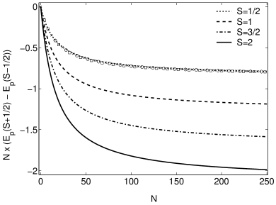
Figure 2: The flow of the energy difference $N\times(E_{p,1}(S+1/2)-E_{p,1}(S-1/2))$ of high-spin and low-spin one-particle excitations for different values of $S$ and ferromagnetic coupling $J=-0.1$. The symbols ($\times$ for $S=1$, $\circ$ for $S=3/2$, and $\scriptsize\square$ for $S=2$) show the flows rescaled by $1/(S+1/2)$.

Figure 2 shows the flows of the energy difference $N\times(E_{p}(S+1/2)-E_{p}(S-1/2))$ for $J=-0.1$ and different values of $S$. The rescaled curves (symbols) show that $A$ and $B(J)$ are indeed independent of $S$. We can obtain the numerical values for $A$ and $B(J)$ by inserting Eq. (14) into Eq. (10) and the result into Eq. (9). Fitting this to the energy difference obtained from the NRG, we obtain a value of $A\approx 1.56\pm 0.01$ independent of $J$ and $S$ for a small $J$. The values for $B(J)$ are given in Table 1.

Our value of $A\approx 1.56$ yields an $\tilde{A}=0.977\approx 1$. Eq. (12) thus simplifies to

$$\tilde{J}(\omega)=1/\ln(\omega/T_{0})\>,$$ (16)

which agrees with the scaling result used for the spin susceptibility in Eq. (72).

J	S=1/2	S=1	S=3/2	S=2
-0.005	1.5990	1.5991	1.5992	1.5994
-0.010	1.6034	1.6036	1.6039	1.6043
-0.025	1.6226	1.6223	1.6219	1.6214
-0.050	1.6637	1.6586	1.6516	1.6426
-0.100	1.7589	1.7270	1.6827	1.6261
-0.200	1.9540	1.7970	1.5789	1.3017

Table 1: Values for $B(J)$ obtained by numerical fitting of the low-energy behaviour (iterations $50-250$) to Eq. (10) and Eq. (14) using $250$ iterations at $\Lambda=3.5$.

In the limit $N\to\infty$, the energy $E_{pp,1}(N,S)$ of the lowest two-particle excitation with quantum numbers $Q=2$ and $S_{\rm tot}=S$ is equal to $2\times E^{(0)}_{p,1}(N)$ of the non-interacting case. The difference $E_{pp,1}(N,S)-2E^{(0)}_{p,1}(N)$ falls off relatively slowly with $N$, approximately as $1/N^{2}$, which we can interpret as a second order effect of $\tilde{J}(N)$.

Following the analysis used by Hofstetter and Zaránd Hofstetter and Zaránd (2004) we can deduce the asymptotic form the phase shifts in the two spin channels, $\eta_{S+1/2}(\omega)$ and $\eta_{S-1/2}(\omega)$, from the energy levels of the low-lying single particle excitations in the approach to the fixed point ($N\to\infty$). The relation of the phase shift to the NRG flows is

$$E_{p,1}(N)=E^{*}_{1}\,\Big{(}1-\tfrac{1}{\pi}\,\eta(N)\Big{)}$$ (17)

with $E^{*}_{1}$ denoting the one-particle excitation energy at the fixed point. Translating the $N$ dependence in a $\omega$ dependence and making use of the fact that $E^{(0)}_{p,1}(N)\to E^{*}_{1}$ very rapidly, we can use Eq. (7) and Eq. (8) to calculate the phase shift. For the $S+1/2$ channel we obtain

$$\eta_{S+1/2}(\omega)=-{\bar{\alpha}_{01}^{2}\over E^{*}_{1}}\pi S\tilde{J}(\omega)$$ (18)

and similarly for the $S-1/2$

$$\eta_{S-1/2}(\omega)={\bar{\alpha}_{01}^{2}\over E^{*}_{1}}\pi(S+1)\,\tilde{J}(\omega)\>.$$ (19)

The numerical value of the proportionality factor is $\bar{\alpha}_{01}^{2}/E^{*}_{1}=0.49$ for a $\Lambda=1.8$. In appendix A we consider explicitly the exchange scattering of a single quasiparticle by an interaction $\tilde{J}$, which should asymptotically describe the behaviour near the fixed point. The resulting phase shifts are given in Eq. (61) and can be seen to give the same as those estimated from the level shifts for $\omega\to 0$ ($\tilde{J}(\omega)\to 0$).

II.2 Antiferromagnetic coupling ($J>0$)

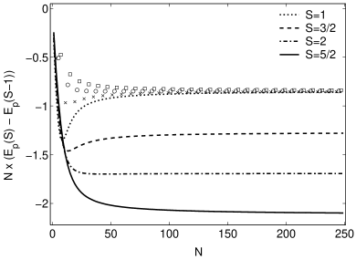
Figure 3: The flow of the energy difference $N\times(E_{p,1}(S)-E_{p,1}(S-1))$ of high-spin and low-spin one-particle excitations for different values of $S$ and antiferromagnetic coupling $J=+0.2$. The symbols ($\times$ for $S=3/2$, $\circ$ for $S=2$, and $\scriptsize\square$ for $S=5/2$) show the flows rescaled by $1/S$.

For antiferromagnetic coupling, a partial screening of the spin $S$ takes place yielding a ground state with a reduced spin $S-1/2$. This screening introduces a phase shift of $\pi/2$, and therefore, in order to facilitate a comparison with the ferromagnetic case, we consider only odd iterations here.

We assume that the low-lying excitations from the ground state can again be expressed using Eq. (4) and calculate $\tilde{J}(N)$ using the flows of the NRG. Figure 3 shows the flow of

$$E_{p,1}(N,S)-E_{p,1}(N,S-1)=\tilde{J}(N)(2S)\alpha_{01}^{2}\Lambda^{(N-1)/2}$$ (20)

multiplied by $N$. This corresponds to the quantity analyzed in the ferromagnetic case as the antiferromagnetic model has a ground state with $S$ replaced with $S-1/2$.

Looking first at the curves for smaller $S$, we see two distinct regions. Initially, $\tilde{J}(N)\times N$ decreases linearly with $N$. For larger values of $N$ we see the flows increasing relatively rapidly. For higher values of $S$, the flow is monotonically decreasing as in the ferromagnetic case. This suggests that the low-energy fixed point is the same as in the ferromagnetic case but with an additional phase shift of $\pi/2$ and a spin $S-1/2$ reduced by $1/2$. Also the approach to the fixed point is formally identical, see Eq. (10) with $S\rightarrow S-1/2$.

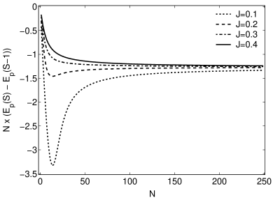
Figure 4: The flow of the energy difference $N\times(E_{p,1}(S)-E_{p,1}(S-1))$ of high-spin and low-spin one-particle excitations for $S=3/2$ different values of the antiferromagnetic coupling $J$.

As can be seen in Fig. 3 and 4, the approach to the fixed point can vary depending on $J$ and $S$. For $T_{0}/D>1$ ($T_{0}/D<1$), the fixed point is approached from below (above). Looking at Fig. 4, we see that for a fixed $S=3/2$ there is a crossover from a non-monotonic flow for smaller values of $J$ to a monotonically decreasing flow for higher values. In the latter case, the flows are completely similar to those with a ferromagnetic bare $J<0$. Therefore it makes sense to use Eq. (14) to define a effective bare $J_{\rm eff}$ for the antiferromagnetic case. We will see below that $J_{\rm eff}$ is usually ferromagnetic. Then, using Eq. (10), the coupling reads

$$\tilde{J}(N)=-\frac{A}{N-B(J)/J_{\rm eff}(J)}\>.$$ (21)

The parameter $J_{\rm eff}$ can be interpreted as an effective coupling between the residual spin and the conduction electrons, provided we are in the strong coupling regime. From Table 1 we infer that in this regime a reasonable approximation to chose a constant $B$. Therefore we use a fixed value $B=1.62$ in order to fit Eq. (21) to the NRG flows (Eq. (20)).

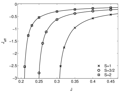
Figure 5: The effective ferromagnetic coupling $J_{\rm eff}$ as a function of the bare antiferromagnetic $J$ for $S=1\,(\times)$, $S=3/2\,(\circ)$, and $S=2\,(\scriptsize\square)$.

The fits yield the same value of $A\approx 1.57$ as in the ferromagnetic case for all $S$ and $J$. The results for $J_{\rm eff}$ as a function of $J$ are plotted in Fig. 5. We observe that $J_{\rm eff}\to 0$ as $J\to\infty$ and that $J_{\rm eff}$ depends strongly on $S$. For smaller values of $J$ than plotted in Fig. 5, $J_{\rm eff}$ is positive and hence the coupling is antiferromagnetic. It should be pointed out, however, that $\tilde{J}(N)$ is always ferromagnetic. This can also be seen in Fig. 4 where all energy differences are negative.

As in the ferromagnetic case, we can derive the phase shifts in the two spin channels. These evaluate to

$$\eta_{S}(\omega)=\frac{\pi}{2}-{\bar{\alpha}_{01}^{2}\over E^{*}_{1}}\pi\big{(}S-\frac{1}{2}\big{)}\,\tilde{J}(\omega)$$ (22)

in the high-spin case and similarly

$$\eta_{S-1}(\omega)=\frac{\pi}{2}+{\bar{\alpha}_{01}^{2}\over E^{*}_{1}}\pi\big{(}S+\frac{1}{2}\big{)}\,\tilde{J}(\omega)$$ (23)

in the low-spin case. The former phase shift agrees with that calculated from the spinon density of states in Ref. Mehta et al., 2004.

III Green’s functions and t matrices

For the calculation of dynamic quantities, we apply the NRG with a discretisation parameter $\Lambda=1.8$ and retain up to $1600$ states. We focus, first of all, on the one-electron Green’s functions and t-matrices. To calculate the t-matrix for the s-d model, we take the equation of motion for the single-electron Green’s function $G_{k\uparrow,k^{\prime}\uparrow}(\omega)={\big{<}\!\big{<}{c^{\phantom{\dagger}}_{k,\uparrow}:c^{\dagger}_{k^{\prime},\uparrow}}\big{>}\!\big{>}}$ and obtain the relation

$$G_{k\uparrow,k^{\prime}\uparrow}(\omega)={\delta_{kk^{\prime}}\over\omega-\epsilon_{k}}+{J\alpha_{k}\over\omega-\epsilon_{k}}\,G_{t}(\omega)\,{J\alpha_{k^{\prime}}\over\omega-\epsilon_{k^{\prime}}}\>,$$ (24)

where $G_{t}(\omega)$ is given by

$$G_{t}(\omega)=\langle\langle S^{-}d^{\phantom{\dagger}}_{\downarrow}+S_{z}d^{\phantom{\dagger}}_{\uparrow}:S^{+}d^{\dagger}_{\downarrow}+S_{z}d^{\dagger}_{\uparrow}\rangle\rangle\>.$$ (25)

Hence in this case the on-shell t-matrixLangreth (1966) can be expressed in terms of the Green’s function $G_{t}(\omega)$ via

$$t_{k,k^{\prime}}(\omega)=J^{2}\,\alpha_{k}\alpha_{k^{\prime}}\,G_{t}(\omega)\;.$$ (26)

We can find a relation between $G_{t}(\omega)$ and the local electron Green’s function $G_{d}(\omega)\equiv{\big{<}\!\big{<}{d^{\phantom{\dagger}}_{\sigma}:d^{\dagger}_{\sigma}}\big{>}\!\big{>}}$ on the $d$ site. For this we multiply Eq. (24) by $\alpha_{k}$ $\alpha_{k^{\prime}}$ and sum over all $k$ and $k^{\prime}$. We find

$$G_{d}(\omega)=G_{d}^{(0)}(\omega)+J^{2}\,G_{d}^{(0)}(\omega)\,G_{t}(\omega)\,G_{d}^{(0)}(\omega)\>,$$ (27)

with the non-interacting $d$-site Green’s function

$$G_{d}^{(0)}(\omega)=\sum_{k}{|\alpha_{k}|^{2}\over{\omega-\epsilon_{k}}}\>.$$ (28)

In the wide band limit we can take $G_{d}^{(0)}(\omega)=-i\pi\rho_{0}$ for $\omega\ll D$, and in this case we find

$$G_{d}(\omega)=-i\pi\rho_{0}-\pi^{2}\rho_{0}^{2}J^{2}G_{t}(\omega)\>.$$ (29)

From this we deduce for the spectral densities

$$\rho_{d}(\omega)=\rho_{0}\big{[}1-\pi^{2}\rho_{0}J^{2}\rho_{t}(\omega)\big{]}\>,$$ (30)

where $\rho_{t}(\omega)=-\textrm{Im}\,G_{t}(\omega)/\pi$.

We know from the results for the Anderson model (see appendix B) that $\rho_{d}(0)=0$. This must apply to the s-d model with antiferromagnetic coupling with spin $S=1/2$, because it is equivalent to the Kondo limit of the Anderson model. By inserting $\rho_{d}(0)=0$ into Eq. (30) we find

$$\rho_{t}(0)={1\over\pi^{2}\rho_{0}J^{2}}\>.$$ (31)

We conjecture that this result applies quite generally for antiferromagnetic coupling and all values of $S$. This is confirmed in our numerical results given below.

III.1 Anderson model and Kondo model

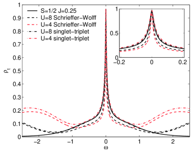
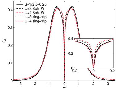
Figure 6: Spectral densities $\rho_{f}$ of the Anderson model and $\rho_{t}$ of the Kondo model (top) as well as $\rho_{d}$ (bottom) for both model; A resonance in $\rho_{f}$ and $\rho_{t}$ corresponds to an antiresonance in  $\rho_{d}$.

In this subsection we look at the relation between the Kondo model (in our notation: s-d model with $S=1/2$ and antiferromagnetic coupling) and the Anderson impurity model. In the latter model the spin $S=1/2$ is replaced with an $f$-level that couples to the conduction band at the site $d$ with hybridization $V$, see Fig. 1. On this $f$-site the electrons interact with a Hubbard repulsion $U$. The Anderson model and the Kondo model are known to be related by the Schrieffer-Wolff transformationSchrieffer and Wolff (1966) which yields $J=4V^{2}/U$.

Another way of relating these two models is to look at the singlet-triplet splitting at the isolated impurity in both cases. For symmetric parameters of the Anderson model this yields

$$J=-\frac{U}{8}+\frac{1}{2}\,\sqrt{\left(\frac{U}{4}\right)^{2}+\,4\,V^{2}}\>.$$ (32)

By expanding the square root to first order in $V^{2}/U^{2}$ one recovers the Schrieffer-Wolff result.

Figure 6 compares the spectra of the two models. The top panel shows $\rho_{t}$ of the Kondo model along with the spectrum $\rho_{f}$ of the local $f$-site Green’s function for two different values of $U$. Dashed lines refer to a value of $V$ as calculated from the Schrieffer-Wolff transformation, whereas dot-dashed lines are for a $V$ as calculated from Eq. (32). One observes that in all cases the central resonance of the Kondo model is well approximated by $\rho_{f}$ of the Anderson model. $V$ from the singlet-triplet splitting, however, yields a slightly better approximation to the Kondo model. Obviously, $\rho_{t}$ of the Kondo model does not show the charge excitations present in the Anderson model’s $\rho_{f}$.

The same can be said for the anti-resonance at the $d$-site shown in the bottom panel of Fig. 6. This anti-resonance is expected from Eq. (30). Again the singlet-triplet splitting yields a somewhat better approximation to the anti-resonance of the Kondo model than the Schrieffer-Wolff result.

III.2 Ferromagnetic Coupling

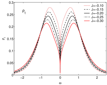
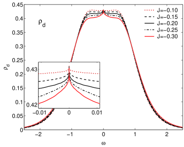
Figure 7: Spectra $\rho_{t}$ (top) and $\rho_{d}$ (bottom) for $S=1/2$ and various values of $J$ for ferromagnetic coupling. The anti-resonance in $\rho_{d}$ corresponds to the resonance in $\rho_{t}$.

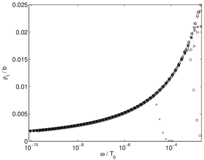
Figure 8: Low-energy behaviour of the rescaled spectral function $\rho_{t}$ as a function of the reduced energy $\omega/T_{0}$ for FM coupling to a spin $S=1/2$. After rescaling, the spectra corresponding to all coupling strengths fall on one curve that is well fitted by $\rho_{t}(\omega)=b/\ln^{2}(T_{0}/\omega)$. The range of fitting is always the interval $[10^{-8},0.5]$ independent of $J$ which takes the values $-0.1\,(\times),-0.15\,(\circ)$ to $-0.45\,(<)$.

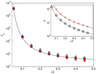
Figure 9: Energy scale $T_{0}$ as a function of the ferromagnetic coupling strength $J$ for different $S$. Estimates of $T_{0}$ from the fit of $\rho_{t}(\omega)=b/\ln^{2}(\omega/T_{0})$ over the interval $[10^{-8},10^{-2}]$ are shown as $(\circ)$ for $S=1/2$ and as $(\times)$ for $S=1$. Estimates of $T_{0}$ from the flows through Eq. (13) are denoted by $\diamond$ for $S=1/2$ and $\ast$ for $S=1$. The full line joining the points is given by $T_{0}(J)=D\,\sqrt{2\rho_{0}J}\,\exp(-1/(2\rho_{0}J))$ with $D=2.55$ and $\rho_{0}=0.47$. In the inset the parameter $b$ is plotted as a function of $J$. Here the data for $S=1$ are roughly $3\,\times$ those for $S=1/2$.

The case of a ferromagnetic coupling to a spin $S=1/2$ is completely different from the antiferromagnetic one, since there is no tendency to screen the impurity spin. There is no corresponding Anderson model.

Qualitatively, the shape of the spectra is reversed, as can be seen in Fig. 7. For ferromagnetic coupling, $\rho_{t}$ has an anti-resonance whereas $\rho_{d}$ a resonance whose height is independentSinjukow et al. (2002) of $J$. This independence stems from the fact that the anti-resonance goes straight down to $\rho_{t}(0)=0$, in which case Eq. (30) implies $\rho_{d}(0)=\rho_{0}$. The low-energy behaviour of $\rho_{t}(\omega)$ can be fitted to the function

$$\rho_{t}(\omega)\sim\frac{b}{\ln^{2}(\omega/T_{0})}$$ (33)

which vanishes at $\omega=0$. This point is illustrated in Fig. 8 where the rescaled spectra for various coupling strengths are plotted on a logarithmic low-energy scale. Equation (33) also reflects the singular approach of $\rho_{t}(\omega)$ to $\omega=0$ as the derivative diverges at this point. This singular behaviour is also seen in the cusp-shaped peak of $\rho_{d}$ at $\omega=0$ (see inset to Fig. 7).

As is shown in Fig. 9, $T_{0}$ seems to be independent of $S$ and can be fitted with the formula

$$T_{0}(J)=D\,\sqrt{2\rho_{0}J}\,e^{-1/(2\rho_{0}J)}$$ (34)

with $D=2.55$ and $\rho_{0}=0.47$. This energy scale agrees remarkably well with the energy scale $T_{0}$ obtained from the fixed point analysis, see Eq. (13). In the ferromagnetic case, $T_{0}$ is a large energy scale and greater than the bandwidth $D$.

III.3 Antiferromagnetic Coupling

We turn to the spectra of the underscreened s-d models with antiferromagnetic coupling to a spin $S>1/2$. Here, a resonance at $\omega=0$ is found in $G_{t}(\omega)$ and an antiresonance in $G_{d}(\omega)$. These are plotted in Fig. 10 for $S=1$ and various values of $J$. The features at $|\omega|\approx 1$ are due to the band edge and $\rho_{t}(0)\approx 1/(J^{2}\pi^{2}\rho_{0})$ as one would expect from Eq. (31). The gap in $\rho_{d}(\omega)$ at $\omega=0$ remains for all $J<0$, and $\rho_{d}(0)=0$ however small $J$ in contrast to the situation $J=0$, where there is no gap and $\rho_{d}(\omega)=\rho_{0}$.

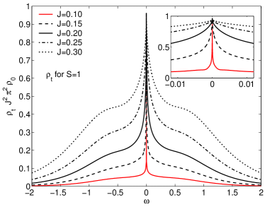
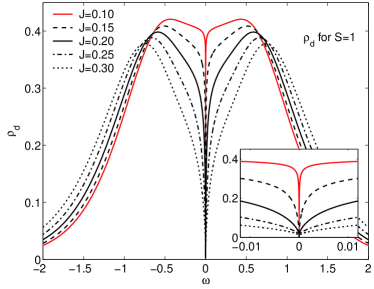
Figure 10: Spectral densities $\rho_{t}$ (top) and $\rho_{d}$ (bottom) of the underscreened s-d model with $S=1$ resonance and antiresonance; former normalized by $J^{2}\pi^{2}\rho_{0}$

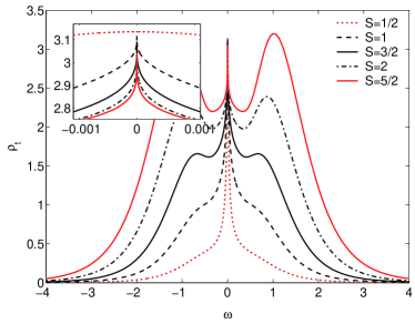
Figure 11: Spectral densities $\rho_{t}$ of the antiferromagnetically coupled s-d model with $S=1/2$ (dotted), $S=1$ (dashed), $S=3/2$, $S=2$ (dot-dashed), and $S=5/2$. The inset shows the resonance on a lower energy scale, where the spectrum of the fully screened model (dotted) is almost flat. The value at $\omega=0$ is approximately the same for all values of $S$.

Figure 11 shows $\rho_{t}(\omega)$ for various values of $S$ and a fixed $J$. The band edge features become more pronounced with increasing $S$, and $\rho_{t}(0)$ is independent of $S$. A magnified picture of the low-energy behaviour is shown in the inset. On this scale, one clearly sees the qualitative difference between the fully screened $S=1/2$ case (quadratic behaviour) and the underscreened $S>1/2$ case (cusps). In the latter case, a good fit to the low-energy behaviour of the spectra $\rho_{t}(\omega)$ can be obtained with

$$\rho_{t}(\omega)\sim a-\frac{b}{\ln^{2}(\omega/T_{0})}\>.$$ (35)

The parameter $a$ is independent of $S$ and approximately given by $a=1/(J^{2}\pi^{2}\rho_{0})$ as inferred from Eq. (30) for a vanishing $\rho_{d}(0)$. In Fig. 12 we plot the rescaled spectra on a logarithmic scale. On low energy scales, all spectra collapse onto a single curve showing (i) the validity of Eq. (35), and (ii) that $b$ is an implicit function of $T_{0}$. The resulting energy scale $T_{0}$ is shown in Fig. 13 as a function of $J$ for various values of $S$. The dashed lines indicate $T_{0}$ as obtained from the flow diagrams. We observe that the agreement of the two approaches to extract $T_{0}$ is not as good as in the ferromagnetic case.

The reason for this disagreement is that these two $T_{0}$’s are obtained from the behaviour on low but rather different energy scales. There is no a priori reason for them to coincide. The antiferromagnetic case is more complex than the ferromagnetic. A higher energy scale (Kondo temperature $T_{K}$, independent of $S$) is associated with the partial screening of the original spin. By contrast, on the lowest energies the residual ferromagnetic coupling leads to another energy scale $T_{0}$ depending on $S$, as discussed in Sec. II. A reasonable explanation of the fact that $T_{0}$ obtained from the spectra differs from the one from the fixed-point analysis is that the former is still affected by the crossover between these regions.

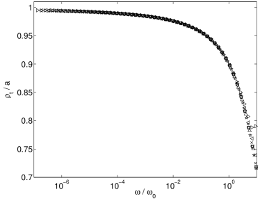
Figure 12: Rescaled spectral densities $\rho_{t}$ of the AFM s-d model with $S=1$ (top) for antiferromagnetic couplings $J=0.1(\times)$, $J=0.15(\circ)$, $\ldots$, $J=0.45$. One sees that after rescaling the spectrum $\rho$ and the frequency $\omega$, all points fall on the same line. For better visibility, the inset shows the same data slightly shifted for each $J$. Full lines are least square fits to $a-b/\ln^{2}(T_{0}/\omega)$. The fits have been done on the interval $[10^{-8},\omega_{0}]$, where $\omega_{0}$ is taken such that $\rho_{t}(\omega_{0})/\rho_{t}(0)\approx 0.9$.

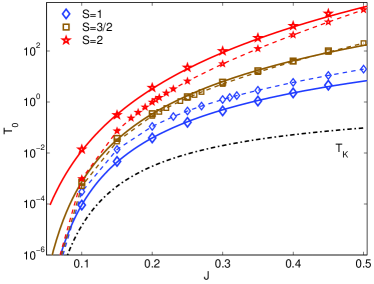
Figure 13: Energy scale $T_{0}$ as a function of the antiferromagnetic coupling $J$ for $S=1$ (diamonds) and $S=3/2$ (squares), and $S=2$ (pentagrams). The full lines show fits to $T_{0}(J)=\bar{D}\,|bJ|^{n}\,\exp(b/J)$ with different values of $\bar{D}$, $b$ and $n$. The dashed lines with the somewhat smaller symbols indicate $T_{0}$ as extracted from the flow diagrams. The dot-dashed line shows $T_{K}=D\,\sqrt{2\rho_{0}J}\exp(-1/(2\rho_{0}J))$ with $D=1$ and $\rho_{0}=0.5$.

IV Scattering Cross Sections

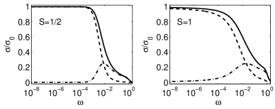
Figure 14: Elastic (dashed), inelastic (dot-dashed) and total (full) cross section for the fully screened model (left) and underscreened model ($S=1$, right) for $J=0.2$.

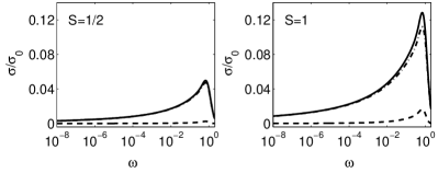
Figure 15: Elastic (dashed), inelastic (dot-dashed) and total (full) cross section for the ferromagnetic model $J=-0.2$ The left-hand (right-hand) plot is for $S=1/2\>(S=1)$. The dot-dashed and the full lines virtually lie on top of each other indicating that the scattering is predominantly inelastic.

The on-shell t-matrix $t_{k,k^{\prime}}$ directly yields the elastic cross section and can be related to the total scattering cross section via the optical theorem. Following Zaránd et al Zaránd et al. (2004), we can write the scattering cross sections as

$$\sigma_{\rm tot}(k) =-\frac{2}{v_{F}}\,\textrm{Im}\,t_{k,k}$$ (36)

$$\sigma_{\rm el}(k) =\frac{1}{v_{F}}\,\int\frac{d^{3}k^{\prime}}{(2\pi)^{3}}\,2\pi\delta(\epsilon_{k^{\prime}}-\epsilon_{k})\,|t_{k^{\prime},k}|^{2}\>,$$

where $v_{F}$ denotes the Fermi velocity. The inelastic cross section is then given by the difference $\sigma_{\rm inel}(k)=\sigma_{\rm tot}(k)-\sigma_{\rm el}(k)$. By evaluating these equations for a flat density of states $\rho_{0}$ and $t_{k^{\prime},k}=J^{2}\,\alpha_{k}\,\alpha_{k^{\prime}}\,G_{t}(\epsilon_{k})$ with $\alpha_{k}$ depending on $k$ only through $\epsilon_{k}$, we obtain

$$\sigma_{\rm tot}(\omega) =-\frac{2J^{2}\,|\alpha_{k}|^{2}}{v_{F}}\,\textrm{Im}\,G_{t}(\omega)$$ (37)

$$\sigma_{\rm el}(\omega) =\frac{2\pi\rho_{0}\,N}{v_{F}}\,J^{4}\,|\alpha_{k}|^{4}\,|G_{t}(\omega)|^{2}\>.$$

This simplifies further if we assume purely isotropic scattering $\alpha_{k}^{2}=1/N$, and we find

$$\sigma_{\rm tot}(\omega) =-\sigma_{0}\rho_{0}\pi\,J^{2}\,\textrm{Im}\,G_{t}(\omega)$$ (38)

$$\sigma_{\rm el}(\omega) =\sigma_{0}\rho_{0}^{2}\pi^{2}\,J^{4}\,|G_{t}(\omega)|^{2}$$ (39)

with $\sigma_{0}^{-1}=\pi\rho_{0}v_{F}N/2$. These cross sections are shown in Fig. 14 for an antiferromagnetic coupling and in Fig. 15 for the ferromagnetic case.

In the antiferromagnetic case, the asymptotic behaviour of $G_{t}(\omega)$ as $\omega\to 0$ is $G_{t}(\omega)\to-i/(\rho_{0}\pi J^{2})$. Therefore, on the Fermi level

$$\sigma_{\rm tot}(0)=\sigma_{\rm el}(0)=\frac{2}{\pi\rho_{0}v_{F}N}\equiv\sigma_{0}\>.$$ (40)

This shows that the inelastic scattering cross section vanishes at the Fermi level, as it should for a Fermi liquid. For the regular Fermi liquid ($S=1/2$, Kondo model), the inelastic scattering vanishes quadratically, and therfore on the lowest energy scale $\sigma_{\rm tot}(\omega)=\sigma_{\rm el}(\omega)$. In contrast to that, for the underscreened model ($S=1$), the inelastic scattering falls off much more slowly.

In the ferromagnetic case, we find that $G_{t}(\omega)\to 0$ as $\omega\to 0$, which implies that the total cross section and thus all scattering vanishes at the Fermi level. Moreover, since $\sigma_{\rm el}(\omega)$ involves the square of $G_{t}(\omega)\ll 1$ for $\omega\to 0$ we expect $\sigma_{\rm el}(\omega)\ll\sigma_{\rm tot}(\omega)\sim G_{t}(\omega)$ which is a formal explanation of the predominance of inelastic scattering in this case.

V Spin Susceptibilities

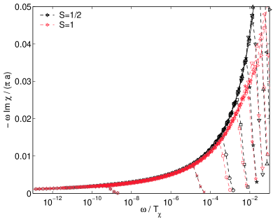
Figure 16: Low-energy spectra of the impurity spin susceptibility multiplied by $\omega$ for ferromagnetic coupling to $S=1/2$ (dark symbols) and $S=1$ (light symbols). The energies are rescaled by $T_{\chi}$ which is fitted from $-\omega\,\textrm{Im}\,\chi(\omega)/\pi=a/\ln^{2}(\omega/T_{\chi})$ with a logarithmic least squares fit. Eq. 43. The ranges of the fits are $[10^{-8}:2\times 10^{-2}]$ for $S=1/2$ and $[10^{-8}:2\times 10^{-3}]$ for $S=1$. $J$ ranges from $J=-0.05(\ast),-0.1(\times),\ldots$ to $J=-0.45(>)$.

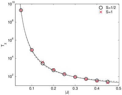
Figure 17: Energy scale $T_{\chi}$ as a function of $J$ for ferromagnetic coupling of a spin $S=1/2(\circ)$ and $S=1(\times)$. The broken line is a fit to Eq. (42) with $a=4.7$ and $b=0.46$. The full line is a better fit to Eq. (42) with $(bJ)^{-1/5}$ instead of the square root and $D=2.55$ and $b=0.50$.

From the NRG we also calculate the impurity spin susceptilibities $\chi(\omega)$ both for ferromagnetic and antiferromagnetic coupling. The low energy behaviour of $\chi(\omega)$ can be obtained from the equations of motion. As is shown in appendix C, the low-energy behaviour is also singular. It goes asymptotically for $\omega\to 0$ as

$$- \frac{1}{\pi}{\rm Im}\langle\langle S_{z}:S_{z}\rangle\rangle=\frac{S(S+1)}{3\omega\ln^{2}(\omega/T_{\chi})}$$ (41)

$$\quad\times\left(1-\frac{\ln(\ln(\omega/T_{\chi}))}{\ln(\omega/T_{\chi})}+{\rm O}\left(\frac{(\ln(\ln(\omega/T_{\chi}))^{2}}{\ln^{2}(\omega/T_{\chi})}\right)\right)\>,$$

where we have introduced an energy scale $T_{\chi}$ which we expect to vary as

$$T_{\chi}=D\,\sqrt{2\rho_{0}|J|}\,e^{-1/(2J\rho_{0})}\>.$$ (42)

This leads to the following ansatz for the low-energy behaviour of the spectrum of $\chi(\omega)$:

$$-\frac{1}{\pi}\,\textrm{Im}\,\chi(\omega)=\frac{a}{\omega\ln^{2}(\omega/T_{\chi})}$$ (43)

Figure 18: Low-energy spectra of the impurity spin susceptibility multiplied by $\omega$ for antiferromagnetic underscreened models $S=1$ (dark symbols) and $S=3/2$ (light red symbols) and $S=2$ (light grey symbols). The energies are rescaled by $T_{\chi}$ which is fitted from $-\omega\,\textrm{Im}\,\chi(\omega)/\pi=a/\ln^{2}(\omega/T_{\chi})$ with a logarithmic least squares fit Eq. (43). The ranges of the fits vary significantly as a function of $J$ to fit the low-energy behaviour. $J$ ranges from $J=0.05(\ast),0.1(\times),\ldots$ to $J=0.45(>)$.

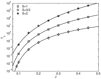
Figure 19: Energy scale $T_{\chi}$ for underscreened s-d models with $S=1\,(\diamond)$, $S=3/2\,(\square)$, and $S=2\,(\star)$. The values of $T_{\chi}$ are obtained from low-energy fits to Eq. (43). Full lines are fits to Eq. (42) with the square root replaced by the exponent $n=2.5$ for $S=1$, $n=5.0$ for $S=3/2$, and $n=7.5$ for $S=2$.

As can be seen from Figs. 16 and 18, this formula describes the low-energy susceptibilities in both the ferromagnetic and the antiferromagnetic cases very well. In the ferromagnetic case, $a\approx S(S+1)/3$ very well with an error of less than $1\%$. In the antiferromagnetic case, $S$ needs to be replaced by $S-1/2$. However, here the agreement is less accurate with an error of the order of $10\%$.

The characteristic energy scale $T_{\chi}$ is plotted in Figs. 17 and 19. We find that $T_{\chi}\approx 2\times T_{0}$ both for ferromagnetic coupling and also for antiferromagnetic coupling, with $T_{0}$ from the fitting of the Green’s functions over the same energy scale.

VI Conclusions

Our NRG calculations give a comprehensive picture of the dynamics of the underscreened and the ferromagnetically coupled impurity s-d models. In the ferromagnetic case, the ground state has $(2S+1)$-fold degeneracy as the impurity spin becomes completely decoupled. The NRG excitations, however, only slowly approach their fixed point values as $1/(N+C(J))$ as $N\to\infty$. This behaviour is consistent with a frequency dependent renormalized exchange coupling $\tilde{J}(\omega)=1/\ln(\omega/T_{0})$, which is a marginally irrelevant operator at this fixed point. The energy scale $T_{0}$, which we calculated in terms of the bare parameters was found to be independent of the spin $S$. Its value, as well as the $T_{\chi}$ deduced from the dynamic susceptibility, corresponds to the usual expression for $T_{K}$, but as $J<0$, it is such that $T_{K}\gg D$.

Essentially the same kind of behaviour was found in the case of the underscreened antiferromagnetic model. After the initial screening of a component of the spin by the conduction electrons in the single channel, the effective spin value is reduced to $S-1/2$. The effective exchange coupling $\tilde{J}(\omega)$ on the low energy scale was also found to be of the form, $\tilde{J}(\omega)=1/\ln(\omega/T_{0})$, and hence is ferromagnetic for $\omega<T_{0}$. The values of $T_{0}$ obtained in this case, however, were found to depend on the spin value $S$, and to be consistently smaller than in the ferromagnetic case, such that $T_{0}\sim D$. The value of $T_{0}$ does not coincide with the formula for the antiferromagnetic $T_{K}$ which is independent of $S$ and always smaller than our values for $T_{0}$. The latter, however, does agree well with the energy scale $T_{\chi}$ deduced from the dynamic susceptibility.

For large values of the bare antiferromagnetic interaction $J$ we were able to estimate the value an effective bare ferromagnetic interaction $J_{\rm eff}$ which would lead to the calculated values of $T_{0}$. From the NRG energy levels in the approach to the fixed point, the asymptotic form of the phase shifts as $\omega\to 0$ due to the elastic scattering of a single particle excitation in the two channels $S_{r}\pm 1/2$ by the residual spin $S_{r}$ could be estimated, where $S_{r}=S$ in the ferromagnetic case and $S_{r}=S-1/2$ for the antiferromagnetic. These were found to be in complete agreement with the values from an explicit calculation of the scattering using the effective low energy Hamiltonian (see Appendix A).

The singular form of the effective coupling $\tilde{J}(\omega)$ is manifest as sharp cusps at the Fermi level in the spectral densities calculated for the Green’s functions $G_{d}(\omega)$ and $G_{t}(\omega)$. For antiferromagnetic coupling the value of $\rho_{t}(\omega)$ at $\omega=0$ was found not to diverge and to approach the value $1/\pi^{2}\rho_{0}J^{2}$ independent of the spin value $S$, as conjectured in Eq. (31). For ferromagnetic coupling the value of $\rho_{t}(0)$ was found to be zero for finite $J$ but equal to $S(S+1)\rho_{0}$ for $J=0$. This clearly demonstrates that $J=0$ is a singular point, and the behaviour is discontinuous as a function of $J$ when $J\to 0$ when approached from the ferromagnetic as well as from the antiferromagnetic side. The approach of $\rho_{d}(\omega)$ and $\rho_{t}(\omega)$ to their values at $\omega=0$ could be described well by terms of the form $1/\ln^{2}(\omega/T_{0})$ in all cases where there is incomplete screening of the local spin. The energy scale deduced from this fitting broadly agrees with the one from the fixed-point analysis. In the case of ferromagnetic coupling the agreement is rather precise.

The results of the calculations for the inelastic and elastic scattering cross-sections as a function of frequency $\omega$ are consistent with the classification of the low energy behaviour of these systems with unscreened residual spins as singular Fermi liquids, as proposed by Mehta et al Mehta et al. (2004). The inelastic scattering goes to zero as $\omega\to 0$ as to be expected for a Fermi liquid, in contrast to non-Fermi liquid behaviour which is characterized by finite inelastic scattering at $\omega=0$. The approach of the inelastic scattering component to zero in the underscreened cases, however, was found to be anomalously slow compared to the corresponding results for the fully screened antiferromagnetic model with $S=1/2$. The singular nature of the low energy scattering is also evident in the contrasting results for the spectral densities of $\rho_{t}(\omega)$ as $\omega\to 0$ in the antiferromagnetic case for $S=1/2$ and $S>1/2$, shown in the inset of Fig. 11. In the case of ferromagnetic coupling, inelastic scattering gives the dominant contribution to the total scattering cross section.

To summarize: our results are in broad agreement with the conclusions of previous studies of the dynamics of underscreened s-d models Parcollet and Georges (1997); Coleman and Pépin (2003); Mehta et al. (2004); Coleman and Paul (2004). However, as well as fully analysing the fixed point behaviour we have been able to make precise predictions for the dynamics of a range of physical response functions, and have also been able to calculate the explicitly the renormalized energy scales $T_{0}$, $T_{\chi}$ etc in terms of the parameters of the bare model.

Appendix A Exchange scattering in the one-electron case

Consider a system of free electrons that couple to a spin $S$ with a local exchange scattering term. The Hamiltonian is given by the sum of Eq. (1) and Eq. (2). We calculate the one-electron states using the basis set $\{{\left|k,\sigma:S,M_{S}\right>}=c^{\dagger}_{k,\sigma}{\left|0\rangle|S,M_{S}\right>}\}$. The Hamiltonian acts on these states as

$$H {\left|k,\uparrow:S,M_{S}\right>}=\epsilon_{k}{\left|k,\uparrow:S,M_{S}\right>}+\alpha_{k}J\sum_{k^{\prime}}\alpha_{k^{\prime}}$$ (44)

$$\times\Big{(}\sqrt{(S-M_{S})(S+M_{S}+1)}\,{\left|k^{\prime},\downarrow:S,M_{S}+1\right>}$$

$$+M_{S}\,{\left|k^{\prime},\uparrow:S,M_{s}\right>}\Big{)}\>.$$

and

$$H {\left|k,\downarrow:S,M_{S}+1\right>}=\epsilon_{k}{\left|k,\downarrow:S,M_{S}+1\right>}+\alpha_{k}J\sum_{k^{\prime}}\alpha_{k^{\prime}}$$

$$\times\Big{(}\sqrt{(S-M_{S})(S+M_{S}+1)}\,{\left|k^{\prime},\uparrow:S,M_{S}\right>}$$

$$-(M_{S}+1)\,{\left|k^{\prime},\downarrow:S,M_{S}+1\right>}\Big{)}\>.$$ (45)

Solving the eigenvalue equation we find the $M_{S}$ dependence cancels out, and the equation factorizes so that we get two independent equations for the new energy levels. With the free $d$-site green’s function as defined in Eq. (28), we obtain

$$1=JS\,G_{d}^{(0)}(\omega)$$ (46)

which corresponds to scattered states in the $S+1/2$ channel and

$$1=-J(S+1)\,G_{d}^{(0)}(\omega)$$ (47)

which correspond to scattering in the $S-1/2$ channel.

The one electron eigenstates in $S+1/2$ channel are built up from the states,

$${\left|k,M_{S}+1/2\right>} =\left({S+M_{S}+1\over 2S+1}\right)^{1/2}{\left|k,\uparrow:S,M_{S}\right>}$$ (48)

$$+\left({S-M_{S}\over 2S+1}\right)^{1/2}{\left|k,\downarrow:S,M_{S}+1\right>}$$

and those for the $S-1/2$ channel from the states,

$${\left|k,M_{S}+1/2\right>} =-\left({S-M_{S}\over 2S+1}\right)^{1/2}{\left|k,\uparrow:S,M_{S}\right>}$$ (49)

$$+\left({S+M_{S}+1\over 2S+1}\right)^{1/2}{\left|k,\downarrow:S,M_{S}+1\right>}$$

We can define corresponding creation operators, $A_{k,M_{S}+1/2}^{\dagger}$ via

$$A_{k,M_{S}+1/2}^{\dagger} =\sqrt{{S+M_{S}+1\over 2S+1}}f(S,M_{S})(S^{+})^{(M_{S}+S)}c_{k,\uparrow}^{\dagger}$$ (50)

$$+\sqrt{{S-M_{S}\over 2S+1}}f(S,M_{S}+1)(S^{+})^{(M_{S}+S+1)}c_{k,\downarrow}$$

where $M_{S}$ can only take values $S,S-1,\ldots,-S-1$ as $(S^{+})^{2S+1}=0$, and $B_{k,M_{S}+1/2}^{\dagger}$ via

$$B_{k,M_{S}+1/2}^{\dagger} =-\sqrt{{S\!-\!M_{S}\over 2S+1}}f(S,M_{S})(S^{+})^{(M_{S}+S)}c_{k,\uparrow}^{\dagger}$$ (51)

$$+\sqrt{{S+M_{S}+1\over 2S+1}}f(S,M_{S}+1)(S^{+})^{(M_{S}+S+1)}c_{k,\downarrow}$$

where $M_{S}$ can take values $S-1,\ldots,-S$. These operators operate on the vacuum state ${\left|0\rangle|S,-S\right>}$, and $f(S,M_{S})$ is a normalization factor such that $f(S,M_{S})(S^{+})^{(M_{S}+S)}{\left|S,-S\right>}={\left|S,M_{S}\right>}$.

Confining our attention to the system with no more than one electron we find equations for the Green’s functions $G^{A}_{k,k^{\prime},M_{S}+1/2}(\omega)={\big{<}\!\big{<}{A_{k,M_{S}+1/2}:A_{k^{\prime},M_{S}+1/2}^{\dagger}}\big{>}\!\big{>}}$ and $G^{B}_{k,k^{\prime},M_{S}+1/2}(\omega)={\big{<}\!\big{<}{B_{k,M_{S}+1/2}:B_{k^{\prime},M_{S}+1/2}^{\dagger}}\big{>}\!\big{>}}$ as

$$(\omega-\epsilon_{k})\, G^{A}_{k,k^{\prime},M_{S}+1/2}(\omega)=\delta_{k,k^{\prime}}$$ (52)

$$+\alpha_{k}JS\sum_{k^{\prime\prime}}\alpha_{k^{\prime\prime}}G^{A}_{k^{\prime\prime},k^{\prime},M_{S}+1/2}(\omega)$$

and

$$(\omega-\epsilon_{k})\, G^{B}_{k,k^{\prime},M_{S}+1/2}(\omega)=\delta_{k,k^{\prime}}$$ (53)

$$- \alpha_{k}J(S+1)\sum_{k^{\prime\prime}}\alpha_{k^{\prime\prime}}G^{B}_{k^{\prime\prime},k^{\prime},M_{S}+1/2}(\omega)\>.$$

Solving these equations we obtain

$$G^{A}_{k,k^{\prime},M_{S}+1/2}(\omega) ={\delta_{k,k^{\prime}}\over\omega-\epsilon_{k^{\prime}}}$$ (54)

$$+{\alpha_{k}\over\omega-\epsilon_{k}}{JS\over 1-JSG_{d}^{(0)}(\omega)}{\alpha_{k^{\prime}}\over\omega-\epsilon_{k^{\prime}}}$$

and

$$G^{B}_{k,k^{\prime},M_{S}+1/2}(\omega) ={\delta_{k,k^{\prime}}\over\omega-\epsilon_{k^{\prime}}}$$ (55)

$$-{\alpha_{k}\over\omega-\epsilon_{k}}{J(S+1)\over 1+J(S+1)G_{d}^{(0)}(\omega)}{\alpha_{k^{\prime}}\over\omega-\epsilon_{k^{\prime}}}\>.$$

This enables us to calculate also the Green’s function $G_{t}(\omega)$ as defined in Eq. (25) for the one-electron case. In terms of the creation and annihilation operators defined in equations (50) and (51), we find

$$S^{+}d^{\dagger}_{\downarrow}+S_{z}d^{\dagger}_{\uparrow}= \sum_{k}{\alpha_{k}\over\sqrt{2S+1}}$$ (56)

$$\times \Big{\{}S\sqrt{S+M_{S}+1}A_{k,M_{S}+1/2}^{\dagger}$$

$$+ (S+1)\sqrt{S-M_{S}}B_{k,M_{S}+1/2}^{\dagger}\Big{\}}\>.$$

The Green’s function $G_{t}(\omega)$ for this one electron situation is then given by

$$G_{t}(\omega) =\sum_{k,k^{\prime},M_{S}}{\alpha_{k}\alpha_{k^{\prime}}\over 2(2S+1)^{2}}$$ (57)

$$\Big{\{}S^{2}(S+M_{S}+1)\,G^{A}_{k,k^{\prime},M_{S}+1/2}(\omega)$$

$$+(S+1)^{2}(S-M_{S})\,G^{B}_{k,k^{\prime},M_{S}+1/2}(\omega)\Big{\}}\>.$$

We find

$$\sum_{k,k^{\prime}}\alpha_{k}\alpha_{k^{\prime}}G^{A}_{k,k^{\prime},M_{S}+1/2}(\omega)={G_{d}^{(0)}(\omega)\over 1-JSG_{d}^{(0)}(\omega)}$$ (58)

and

$$\sum_{k,k^{\prime}}\alpha_{k}\alpha_{k^{\prime}}G^{B}_{k,k^{\prime},M_{S}+1/2}(\omega)={G_{d}^{(0)}(\omega)\over 1+J(S+1)G_{d}^{(0)}(\omega)}\>.$$ (59)

We substitute these into Eq. (57) and perform the sums over $M_{S}$. This sum has to be done carefully because the for the first term the sum is over the values $-S-1,-S,\ldots,S$, whereas for the second term it is over $-S,-S+1,\ldots,S-1$. The result is

$$G_{t}(\omega) ={S(S+1)G_{d}^{(0)}(\omega)\over 2}$$ (60)

$$\times\left\{{1\over 1-JSG_{d}^{(0)}(\omega)}+{1\over 1+J(S+1)G_{d}^{(0)}(\omega)}\right\}\>.$$

In our many-electron case this theory is only directly applicable in the immediate vicinity of the fixed point with one quasiparticle excited from the interacting ground state and $J$ interpreted as the renormalized coupling $\tilde{J}$. The phase shifts for the quasiparticle scattering are then given by

$$\eta_{S+1/2}(\omega) =-\arctan\big{(}\pi\rho_{0}(\omega)\tilde{J}(\omega)S\big{)}\>,$$ (61)

$$\eta_{S-1/2}(\omega) =\quad\arctan\big{(}\pi\rho_{0}(\omega)\tilde{J}(\omega)(S+1)\big{)}$$

with $\tilde{J}(\omega)=1/\ln(\omega/T_{0})$. In the limit $\omega\to 0$, the phase shifts we calculate in this way agree with the estimates Eq. (18) and Eq. (19) obtained from the NRG flows.

Appendix B Green’s Functions and t-Matrices for the Anderson Model

Let the impurity site be labelled by $f$ and next site it is coupled to on the chain be labelled $d$, as indicated in Fig. 1. Let $d_{\sigma}=\sum_{k}V_{k}c_{k}/V$ where $|V|^{2}=\sum_{k}|V_{k}|^{2}$. The equation of motion for the Green’s function $G_{kk^{\prime}}(\omega)$ yields the relation

$$G_{kk^{\prime}}(\omega)={\delta_{kk^{\prime}}\over\omega-\epsilon_{k}}+{V\alpha_{k}\over\omega-\epsilon_{k}}\,G_{f}(\omega)\,{V\alpha_{k^{\prime}}\over\omega-\epsilon_{k}^{\prime}}\>.$$ (62)

The t-matrix $t_{kk^{\prime}}(\omega)$ is defined by the equation,

$$G_{kk^{\prime}}(\omega)={\delta_{kk^{\prime}}\over\omega-\epsilon_{k}}+{1\over\omega-\epsilon_{k}}\,t_{kk^{\prime}}(\omega)\,{1\over\omega-\epsilon_{k}^{\prime}}\>,$$ (63)

and hence for the Anderson model we have

$$t_{kk^{\prime}}(\omega)=V^{2}\alpha_{k}G_{f}(\omega)\alpha_{k^{\prime}}\>.$$ (64)

We can derive an expression for $G_{d}(\omega)$ from $G_{kk^{\prime}}(\omega)$ by multiplying by $V_{k}$, $V_{k^{\prime}}$, and summing over $k$ and $k^{\prime}$. This gives

$$G_{d}(\omega)=G_{d}^{(0)}(\omega)+V^{2}G_{d}^{(0)}(\omega)\,G_{f}(\omega)\,V^{2}\,G_{d}^{(0)}(\omega)\>.$$ (65)

In the wide band limit $V^{2}\,G_{d}^{(0)}(0)=-i\Delta$ and hence,

$$G_{d}(\omega)={1\over V^{2}}\,\left[-i\Delta-\Delta^{2}G_{f}(\omega)\right]\>.$$ (66)

We can deduce the spectral density of $G_{d}(\omega)$ from

$$\rho_{d}(\omega)=-{1\over\pi}{\textrm{Im}\,}G_{f}(\omega)=\rho_{0}[1-\pi\Delta\rho_{f}(\omega)]\>,$$ (67)

where we have used the result $\Delta=\pi\rho_{0}|V|^{2}$, where $\rho_{0}$ is the free conduction density of states at the Fermi level. It follows from this expression that for the symmetric model, where $\rho_{f}(0)=1/\pi\Delta$, the spectral density of $G_{d}$ vanishes, $\rho_{d}(0)=0$. Therefore, we find an anti-resonance.

Appendix C Dynamic Spin susceptibility

We derive equations of motion for the local spin-spin double-time Green’s function $\langle\langle S^{+}(t):S^{-}(t^{\prime})\rangle\rangle$ to second order in the coupling $J$. For this we need the evaluation of the higher order Green’s function to zero order only. We find from the equations of motion

$$\omega^{2}\langle\langle S^{+}:S^{-}\rangle\rangle_{\omega}={8J^{2}S(S+1)\over 3}\langle\langle S_{d}^{+}:S_{d}^{-}\rangle\rangle_{\omega}\>,$$ (68)

where we have used the fact the $\langle\langle S^{+}:S^{-}\rangle\rangle=2\langle\langle S_{z}:S_{z}\rangle\rangle$, due to the rotational symmetry in zero magnetic field. The spin operator $S_{d}^{+}$ for the first site on the chain in terms of the conduction electron states is given by $S_{d}^{+}=d^{\dagger}_{\uparrow}d^{\phantom{\dagger}}_{\downarrow}=\sum_{k,k^{\prime}}\alpha_{k}\alpha_{k^{\prime}}c^{\dagger}_{k\uparrow}c^{\phantom{\dagger}}_{k^{\prime}\downarrow}$, with a similar expression for $S_{d}^{-}$. Evaluation of $\langle\langle S_{d}^{+}:S_{d}^{-}\rangle\rangle$ to zero order in $J$ gives

$$\langle\langle S_{d}^{+}:S_{d}^{-}\rangle\rangle=\int\!\!\!\!\int\rho_{0}(\epsilon)\rho_{0}(\epsilon^{\prime})\left({f(\epsilon)-f(\epsilon^{\prime})\over\omega-\epsilon^{\prime}+\epsilon}\right)\,d\epsilon\,d\epsilon^{\prime}\>,$$ (69)

where $\rho_{0}(\omega)=\sum_{k}\alpha_{k}^{2}\delta(\omega-\epsilon)$ is the local spectral density for the first site on the chain for the non-interacting system. From that we deduce that the spectral density of $\langle\langle S^{+}:S^{-}\rangle\rangle$ to order $J^{2}$ is given by

$$-{1\over\pi} {{\rm Im}\langle\langle S^{+}:S^{-}\rangle\rangle}={8J^{2}S(S+1)\over 3\,\omega^{2}}$$ (70)

$$\times\int\rho_{0}(\epsilon)\rho_{0}(\epsilon+\omega)(f(\epsilon)-f(\epsilon+\omega))\,d\epsilon\>.$$

For the limit $\omega\to 0$ we find

$$-{1\over\pi}\lim_{\omega\to 0}\omega\,\textrm{Im}\,\langle\langle S^{+}:S^{-}\rangle\rangle={8(J\rho_{0}(0))^{2}S(S+1)\over 3}$$ (71)

Using the poor man’s scaling equation, Eq. (3.51) in Ref. Hewson, 1993, with $\tilde{D}=a\,\omega$, the coupling $J$ is renormalized to $\tilde{J}(\omega)$ given by

$$2\tilde{J}\rho_{0}={1\over\ln(\omega/T_{\chi})}-{\ln(\ln(\omega/T_{\chi})\over 2\ln^{2}(\omega/T_{\chi})}+{\rm O}\left({1\over\ln^{2}(\omega/T_{\chi})}\right)\>,$$ (72)

with the energy scale $T_{\chi}$ given by

$$T_{\chi}=D|2J\rho_{0}|^{1/2}e^{-1/2J\rho_{0}}\>.$$ (73)

Hence, asymptotically as $\omega\to 0$,

$$- \frac{1}{\pi}{\rm Im}\langle\langle S^{+}:S^{-}\rangle\rangle=\frac{2S(S+1)}{3\omega\ln^{2}(\omega/T_{\chi})}$$ (74)

$$\times\left(1-\frac{\ln(\ln(\omega/T_{\chi}))}{\ln(\omega/T_{\chi})}+{\rm O}\left(\frac{(\ln(\ln(\omega/T_{\chi}))^{2}}{\ln^{2}(\omega/T_{\chi})}\right)\right)\>.$$

For the fully screened Kondo model, this asymptotic form should be appropriate only for the regime $D>\omega>T_{\chi}=T_{K}$. However, for a ferromagnetic coupling and for the underscreened models, this asymptotic form should also apply as $\omega\to 0$, as confirmed in Sec. V. As the asymptotic behaviour of the underscreened models is associated with a ferromagnetic fixed point, the low-temperature $T_{\chi}$ is expected to differ from $T_{K}$ (high temperature), see Sec. V.