Statistical mechanics of general discrete nonlinear Schrödinger models: Localization transition and its relevance for Klein-Gordon lattices

Abstract

We extend earlier work [Phys. Rev. Lett. 84, 3740 (2000)] on the statistical mechanics of the cubic one-dimensional discrete nonlinear Schrödinger (DNLS) equation to a more general class of models, including higher dimensionalities and nonlinearities of arbitrary degree. These extensions are physically motivated by the desire to describe situations with an excitation threshold for creation of localized excitations, as well as by recent work suggesting non-cubic DNLS models to describe Bose-Einstein condensates in deep optical lattices, taking into account the effective condensate dimensionality. Considering ensembles of initial conditions with given values of the two conserved quantities, norm and Hamiltonian, we calculate analytically the boundary of the ’normal’ Gibbsian regime corresponding to infinite temperature, and perform numerical simulations to illuminate the nature of the localization dynamics outside this regime for various cases. Furthermore, we show quantitatively how this DNLS localization transition manifests itself for small-amplitude oscillations in generic Klein-Gordon lattices of weakly coupled anharmonic oscillators (in which energy is the only conserved quantity), and determine conditions for existence of persistent energy localization over large time scales.

I Introduction

There is a large interest in many branches of current science in the topic of localization and energy transfer in Hamiltonian nonlinear lattice systems (see e.g. Ref. Flach for a comprehensive review, and Refs. escorial ; Chaos ; PW for more recent progress). Under quite general conditions, such lattices sustain exact, spatially exponentially localized and time-periodic, solutions termed intrinsically localized modes (ILMs) or discrete breathers (DBs). Although their existence as exact solutions has been rigorously proven in many explicit cases (MacKay ; Aubry , and e.g. Ref. AKK01 ; James03 ; JN03 and references therein for extensions), there is still an ongoing debate regarding their relevance to actual physical phenomena, at nonzero temperatures. Important fundamental questions concern whether ILMs may exist in thermal equilibrium, or if not, whether their typical lifetimes are long enough to considerably influence transport properties of crystals, biomolecules, etc.

A frequently studied example of a non-integrable Hamiltonian lattice model is the discrete nonlinear Schrödinger (DNLS) equation (see Refs. KRB01 ; EJ for recent reviews of its history, properties and applications). This model is of great interest from a general nonlinear dynamics point of view, where it provides a particularly simple system to analyze fundamental phenomena such as energy localization, wave instabilities etc., resulting from competition of nonlinearity and discreteness, as well as from a more applied viewpoint describing e.g. arrays of nonlinear optical waveguides or Bose-Einstein condensates in external periodic potentials. The DNLS equation can be derived through an expansion on multiple time-scales of small-amplitude oscillations in a generic class of weakly coupled anharmonic oscillators [Klein-Gordon (KG) lattice], and thus approximates the KG dynamics over large but finite time-ranges (see, e.g., Refs. Flach ; Peyrard ; Morgante ). A particular feature of the DNLS model is the existence of a second conserved quantity in addition to the Hamiltonian: the total excitation number (norm) of the solution. In the KG model, this quantity roughly corresponds to the total action integral, which thus must be an approximate invariant in cases where the DNLS description of the KG dynamics is acceptable.

A fundamental question is, for which kinds of spatially extended initial states may we expect spontaneous formation of persistent localized modes in such lattices? The answer generally requires a statistical-mechanics description of the model. Due to the existence of a second conserved quantity, it has been possible to obtain some analytical results for the thermodynamic properties of the DNLS model in the grand-canonical ensemble, by identifying the norm with the number of particles in the standard Gibbsian approach (this is also its physically relevant interpretation in the Bose-Einstein DNLS realization). In Ref. RCKG00 , it was found that the onset of persistent localization could be identified with a phase transition line in parameter space, such that on one side the system thermalized according to the Gibbsian distribution with well-defined chemical potential and (positive) temperature, while on the other side the dynamics was associated with a negative-temperature behavior (for finite systems) creating a small number of large-amplitude, standing localized breathers. The transition line was shown to correspond to the limit of infinite temperatures in the ’normal’ regime. Similar properties were later found also for other types of lattice models with two conserved quantities in Ref. RN . Most recently, in Ref. Rumpf Rumpf revisited the statistical-mechanics description of the DNLS localization transition. Under the particular assumption of small-amplitude initial conditions (an assumption not made in Ref. RCKG00 ), he argues that the phase space generally can be divided into two weakly interacting domains, corresponding to low-amplitude fluctuations (’phonons’) and high-amplitude peaks (breathers), respectively. Explicit expressions for macroscopic quantities, valid not only in the ’normal’ regime but in the full range of parameter space, can then be obtained by assuming the two domains to be in thermal equilibrium with each other, and the emergence of localized peaks in the ’anomalous’ phase arises as the system strives for maximizing its total entropy. Under these conditions, the temperature is not negative but infinite in the thermal equilibrium state with coexisting large-amplitude breathers and small-amplitude fluctuations.

Let us mention a number of reasons that have lead us to revisit and extend the results of Ref. RCKG00 . First, so far only the one-dimensional (1D) case with cubic nonlinearity was considered. However, apart from the natural interest in considering two- and three-dimensional (2D and 3D) physical situations, there is also a fundamental difference to the 1D case: there is an excitation threshold for creation of localized excitations for the cubic DNLS model FKM97 ; W99 ; KRB00 . A similar threshold also occurs in the 1D DNLS equation for noncubic nonlinearities of the form $|\psi_{m}|^{2\sigma}\psi_{m}$ with $\sigma>2$ FKM97 ; W99 ; KRB00 , and generally the condition $\sigma D>2$ for existence of an excitation threshold in $D$ dimensions is the same as the condition for collapse of the ground-state solution of the corresponding continuous NLS equation (e.g. Ref. RR86 ). For this reason, one sometimes studies the 1D DNLS equation with larger $\sigma$ hoping to capture the main effects of higher dimensionality in a simpler 1D model (e.g. Refs. BRC94 ; Laedke ; Usero ; BM00 ). Recently EFT03 , similar arguments were also used in the study of a 1D KG chain with a $\phi^{8}$ on-site potential, to mimic the effects of an excitation threshold for breathers in the thermalization dynamics of a three-dimensional KG-lattice. (A similar relation between degree of nonlinearity and dimension is valid also for KG-lattices, see Ref. FKM97 , and Ref. Kastner for recent extensions.) Thus, it is of interest to investigate the nature of the statistical localization transition for various degrees of nonlinearity and dimensions, in order to elucidate (i) whether it is qualitatively affected by the existence of a breather excitation threshold, and (ii) whether quantitative effects arising from increasing $\sigma$ agree with those from increasing $D$.

While the above connection motivates the study of particular on-site nonlinearities with $\sigma=2$ and $\sigma=3$, recent progress in studies of Bose-Einstein condensates in optical lattices also provide motivation for considering non-integer values of $\sigma<1$. It has namely been suggested Smerzi , that the effective power of the nonlinearity in the tight-binding DNLS approximation depends on the effective dimensionality $d$ of the condensate in each well, such that $\sigma=2/(2+d)$ where $d=0,1,2$, or 3. Moreover, it is tempting to suggest a connection between the statistical localization transition in the DNLS model and experimentally observed superfluid-insulator transitions of the condensate (e.g. Refs. Greiner ; Cataliotti and references therein).

Last, but not least, we wish to employ the results for the DNLS model to give quantitative predictions for breather formation in generic KG models, and in particular describe what kinds of initial conditions yield long-lived breathers in the regime of weak coupling and small averaged energy density where the DNLS approximation is justified. Although particular examples of the manifestation of the DNLS localization transition in KG models have been given earlier Morgante , we here derive explicit general approximate expressions for the transition line in terms of direct properties of the KG initial state. Due to the violation of norm (or action) conservation, the transition in the KG model is not strict, and we perform numerical simulations to investigate how the long-time dynamics is influenced by the slow variation of the almost conserved quantity. We suggest that the approach proposed here could be used to clarify the findings regarding the role of breathers in thermalized KG lattices (with or without energy gaps) of Refs. EFT03 ; ET , which did not employ the connection to the DNLS model.

The structure of this paper is as follows. Sec. II describes the statistical mechanics of general DNLS models. Sec. II.1 generalizes the statistical-mechanics approach of Ref. RCKG00 to 1D models with general degrees of nonlinearity. As particular examples, we consider initial conditions taken as traveling (Sec. II.1.1) and standing (Sec. II.1.2) waves. We obtain simple analytical conditions for the transition into the statistical localization regime, and illustrate with numerical simulations the actual dynamics on both sides of the transition. Sec. II.2 extends these results to higher dimensions. In Sec. III we describe how the results from the DNLS model can be transfered into approximate conditions for statistical formation of long-lived breathers in weakly coupled Klein-Gordon chains, and confirm and illuminate these predictions with numerical simulations. Sec. IV gives some concluding remarks and perspectives.

II Statistical mechanics of general DNLS models

II.1 1D model with general degree of nonlinearity

Generalizing the 1D DNLS equation of Ref. RCKG00 to include a nonlinearity of arbitrary (homogeneous) degree, we consider the DNLS equation in the form:

$$i\dot{\psi}_{m}+C(\psi_{m+1}+\psi_{m-1})+|\psi_{m}|^{2\sigma}\psi_{m}=0,$$ (1)

with the two conserved quantities Hamiltonian ${\mathcal{H}}=\sum_{m}\left[C(\psi_{m}\psi_{m+1}^{\ast}+\psi_{m}^{\ast}\psi_{m+1})+\frac{1}{\sigma+1}|\psi_{m}|^{2\sigma+2}\right]$, and norm (excitation number) ${\cal A}=\sum_{m}|\psi_{m}|^{2}$. Compared to Eq. (1) of Ref. RCKG00 , we have used $\nu=1$ as the coefficient of the nonlinear term, included a coupling constant $C>0$ in front of the coupling terms, and generalized $|\psi_{m}|^{2}\psi_{m}$ to $|\psi_{m}|^{2\sigma}\psi_{m}$ with $\sigma>0$. Note that although we formally discuss the case of positive intersite coupling and positive nonlinearity, this is not a restriction, since changing the sign of $C$ is equivalent to the transformation $\psi_{m}\rightarrow(-1)^{m}\psi_{m}$, while the same transformation followed by a time reversal $t\rightarrow-t$ is equivalent to changing the sign of the nonlinearity. Thus, all obtained results can be directly transformed to the cases of negative coupling and/or negative nonlinearity. Any finite coefficient in front of the nonlinear term can also be obtained through a simple rescaling.

With a canonical transformation into action-angle variables, $\psi_{m}=\sqrt{A_{m}}e^{i\phi_{m}}$, the Hamiltonian for a chain of $N$ sites becomes

$${\mathcal{H}}=\sum_{m=1}^{N}\left(2C\sqrt{A_{m}A_{m+1}}\cos(\phi_{m}-\phi_{m+1})+\frac{1}{\sigma+1}A_{m}^{\sigma+1}\right),$$ (2)

and the norm

$${\mathcal{A}}=\sum_{m=1}^{N}A_{m}.$$ (3)

We first note that the staggered ($q=\pi$) stationary homogeneous plane-wave solution $\psi_{m}^{(min)}=\sqrt{{\mathcal{A}}/N}e^{im\pi}e^{i\Lambda t}$, with $\Lambda=-2C+({\mathcal{A}}/N)^{\sigma}$, minimizes ${\mathcal{H}}$ at fixed ${\mathcal{A}}$ and $N$, for all $\sigma$. The minimum value is thus ${\mathcal{H}}^{(min)}=-2C{\mathcal{A}}+\frac{1}{\sigma+1}{\mathcal{A}}^{\sigma+1}/N^{\sigma}$. To prove this, write

$${\mathcal{H}}-{\mathcal{H}}^{(min)}=\sum_{m=1}^{N}\left[2C\left(\sqrt{A_{m}A_{m+1}}\cos(\phi_{m}-\phi_{m+1})+\frac{\mathcal{A}}{N}\right)+\frac{1}{\sigma+1}\left(A_{m}^{\sigma+1}-\left(\frac{\mathcal{A}}{N}\right)^{\sigma+1}\right)\right].$$

The first part is positive, since $\sum\left(\sqrt{A_{m}A_{m+1}}\cos(\phi_{m}-\phi_{m+1})+\frac{\mathcal{A}}{N}\right)\geq\sum\left(\frac{\mathcal{A}}{N}-\sqrt{A_{m}A_{m+1}}\right)=\frac{1}{2}\sum\left(\sqrt{A_{m}}-\sqrt{A_{m+1}}\right)^{2}\geq 0$. The second part is also positive, which can be seen from Hölder’s inequality: $\sum|a_{k}b_{k}|\leq\left(\sum|a_{k}|^{p}\right)^{1/p}\left(\sum|b_{k}|^{q}\right)^{1/q}$, if $1/p+1/q=1$. Let $a_{k}=A_{m},b_{k}=1,p=\sigma+1,q=1+1/\sigma$, which gives $\sum A_{m}^{\sigma+1}-\frac{1}{N^{\sigma}}\left(\sum A_{m}\right)^{\sigma+1}\geq 0$. Notice also that ${\mathcal{H}}^{(min)}$ is bounded from below as a function of $\mathcal{A}$ for any finite number of sites $N$, with the global minimum ${\mathcal{H}}^{(min)}=-\frac{\sigma}{\sigma+1}N(2C)^{1+1/\sigma}$ obtained for ${\mathcal{A}}=N(2C)^{1/\sigma}$.

Similarly to the work of Ref. RCKG00 , we use standard Gibbsian statistical mechanics to predict macroscopic average values in the thermodynamic limit, by treating the norm ${\mathcal{A}}$ as analogous to ’number of particles’ in the grand-canonical ensemble. As in Eq. (2) in Ref. RCKG00 , the grand-canonical partition function is thus defined as

$${\mathcal{Z}}=\int_{0}^{\infty}\int_{0}^{2\pi}\prod_{m=1}^{N}d\phi_{m}dA_{m}e^{-\beta({\mathcal{H}}+\mu{\mathcal{A}})},$$ (4)

where $\beta\equiv 1/T$ (in units of $k_{B}\equiv 1$) and $\mu$ play the roles of inverse temperature and chemical potential, respectively. Using (2)-(3) and integrating over the phase variables $\phi_{m}$ yields

$${\mathcal{Z}}=(2\pi)^{N}\int_{0}^{\infty}\prod_{m}dA_{m}I_{0}(2\beta C\sqrt{A_{m}A_{m+1}})e^{-\beta A_{m}\left(\frac{A_{m}^{\sigma}}{\sigma+1}+\mu\right)},$$ (5)

where $I_{0}(z)=\frac{1}{\pi}\int_{0}^{\pi}e^{zcos\theta}d\theta$ is the modified Bessel function of the first kind. From this expression, one could proceed as in Ref. RCKG00 by symmetrizing the partition function and using the transfer integral operator to obtain thermodynamic quantities in the limit $N\rightarrow\infty$, corresponding to the regime in $({\mathcal{A}},{\mathcal{H}})$ parameter space with well-defined chemical potential and (positive) temperature. This is however not our main purpose here. Instead, we focus on the phase transition line defined by the boundary of this regime ($\beta=0,\mu=\infty$, with $\beta\mu\equiv\gamma$ finite), which signals the transition into the regime of persistent localization, suggested in Ref. RCKG00 to be associated with a negative-temperature type behavior for finite lattices and time-scales.

Close to the high-temperature limit $\beta\rightarrow 0^{+}$, we can approximate the slowly increasing Bessel function with $I_{0}\approx 1$ (which is mathematically equivalent to letting $C\rightarrow 0$, corresponding physically to thermalized independent units). The partition function then becomes ${\mathcal{Z}}\simeq(2\pi y(\beta,\mu))^{N}$, where

$$y(\beta,\mu)=\int_{0}^{\infty}e^{-\beta\mu x}e^{\frac{-\beta x^{\sigma+1}}{\sigma+1}}dx=\int_{0}^{\infty}e^{-\beta\mu x}\left[1-\frac{\beta x^{\sigma+1}}{\sigma+1}+\frac{1}{2}\left(\frac{\beta x^{\sigma+1}}{\sigma+1}\right)^{2}+...\right]dx$$

$$=\frac{1}{\beta\mu}-\frac{\beta}{\sigma+1}\int_{0}^{\infty}x^{\sigma+1}e^{-\beta\mu x}dx+\frac{1}{2}\frac{\beta^{2}}{(\sigma+1)^{2}}\int_{0}^{\infty}x^{2(\sigma+1)}e^{-\beta\mu x}dx+...$$

But $\int_{0}^{\infty}x^{n}e^{-ax}dx=\frac{\Gamma(n+1)}{a^{n+1}}$ (where $\Gamma$ is the Gamma function, $\Gamma(n+1)=n!$ for integer $n$). This yields

$$y(\beta,\mu)=\frac{1}{\beta\mu}-\frac{\beta}{\sigma+1}\frac{\Gamma(\sigma+2)}{(\beta\mu)^{\sigma+2}}+\frac{1}{2}\frac{\beta^{2}}{(\sigma+1)^{2}}\frac{\Gamma(2\sigma+3)}{(\beta\mu)^{2\sigma+3}}+...$$

Thus, close to the limit of $\beta\rightarrow 0,\mu\rightarrow\infty$ with $\beta\mu=\gamma$ constant, we can neglect all higher-order terms in $\beta$, and obtain $y(\beta,\mu)\simeq\frac{1}{\beta\mu}-\frac{\beta\Gamma(\sigma+1)}{(\beta\mu)^{\sigma+2}}$. Finally, for the partition function in the high-temperature limit we get

$${\mathcal{Z}}\simeq(2\pi)^{N}\frac{1}{(\beta\mu)^{N}}\left(1-\frac{\beta\Gamma(\sigma+1)}{(\beta\mu)^{\sigma+1}}\right)^{N}.$$ (6)

For small $\beta$ this reduces to $\ln{\mathcal{Z}}\simeq N\ln(2\pi)-N\ln(\beta\mu)-N{\frac{\beta\Gamma(\sigma+1)}{{(\beta\mu)}^{\sigma+1}}}$, so that we have in the high-temperature limit for the average energy:

$$<{\mathcal{H}}>=\left(\frac{\mu}{\beta}\frac{\partial}{\partial\mu}-\frac{\partial}{\partial\beta}\right)\ln{\mathcal{Z}}\simeq\frac{N\Gamma(\sigma+1)}{(\beta\mu)^{\sigma+1}},$$ (7)

and for the average norm

$$<{\mathcal{A}}>=-\frac{1}{\beta}\frac{\partial\ln{\mathcal{Z}}}{\partial\mu}\simeq\frac{N}{\beta\mu}-\frac{N\Gamma(\sigma+2)}{\mu(\beta\mu)^{\sigma+1}}.$$ (8)

(The second term here is negligible.) Thus, the relation between the energy density $h\equiv\frac{<{\mathcal{H}}>}{N}$ and the norm density $a\equiv\frac{<{\mathcal{A}}>}{N}$ in the high-temperature limit is

$$h=\Gamma(\sigma+1)a^{\sigma+1},$$ (9)

where $\Gamma(\sigma+1)$ can be replaced by $\sigma!$ for integer $\sigma$. Note that the quantity $\gamma=\beta\mu$ indeed is well-defined and finite in the high-temperature limit for any nonzero norm density, $\gamma\simeq 1/a$ according to (8).

For $\sigma=1$, the corresponding phase diagram was illustrated in Fig. 1 of Ref. RCKG00 . Thus, for any given norm density $a$, typical initial conditions with (Hamiltonian) energy density $h$ smaller than the critical value (9) are expected to thermalize (after ’sufficiently’ long times) according to a Gibbsian equilibrium distribution at temperature $T=1/\beta$ and chemical potential $\mu$. The correspondence between $(a,h)$ and $(\beta,\mu)$ generally has to be found numerically through the transfer integral formalism as in Ref. RCKG00 , but in the small-amplitude limit $a\rightarrow 0$ analytic expressions can be obtained as shown in Ref. Rumpf , Eqs. (7)-(8). Numerical evidence that such a thermalization generally takes place after sufficiently long integration times was given in Fig. 2 of Ref. RCKG00 (for $\sigma=1$).

On the other hand, for initial conditions with energy density $h$ larger than the critical value (9) this description breaks down, and one finds numerically that persistent large-amplitude standing breathers are created. Heuristically, this can be understood as follows: For fixed norm ${\mathcal{A}}$, it is generally possible to maximize the Hamiltonian ${\mathcal{H}}$, and the maximizing solution is a single-site peaked, exponentially localized stationary standing breather (see, e.g., Ref. W99 ), which for large ${\mathcal{A}}$ becomes essentially localized at one site so that ${\mathcal{H}}^{(max)}\simeq{\mathcal{A}}^{\sigma+1}/{(\sigma+1)}$. Considering in the microcanonical ensemble (fixed ${\mathcal{A}},{\mathcal{H}}$ and $N$) the entropy $S({\mathcal{H}},{\mathcal{A}},N)$ (i.e. the logarithm of the number of microstates) as a function of ${\mathcal{H}}$, it is zero at ${\mathcal{H}}^{(min)}({\mathcal{A}},N)$ defined above, increases towards its maximum when (9) is fulfilled and $T=\infty$ (since $1/T=\partial S/\partial{\mathcal{H}}|_{{\mathcal{A}},N}$), and then again decreases towards zero at ${\mathcal{H}}^{(max)}({\mathcal{A}})$. Thus, in the microcanonical ensemble at finite ${\mathcal{A}}$ and $N$, the temperature is well-defined and becomes negative when $h={\mathcal{H}}/N$ is larger than the critical value (9). Returning to the grand-canonical ensemble, it is then possible for the part of the system which is in the negative-temperature regime to increase its entropy by transferring some of its superfluous energy into localized breathers, which consume only a small amount of the norm. In other words, the ’overheated’ negative-temperature system ’cools itself off’ by creating breathers as ’hot spots’ of localized energy. Such a mechanism for energy localization works quite generally in systems with two conserved quantities (see, e.g., Ref. RN and references therein). Indeed, this type of argument could be used to explicitly calculate the thermodynamic properties of the DNLS model in the limit of small $a$, where phase space naturally divides into a small-amplitude ’fluctuation’ part and a large-amplitude ’breather’ part Rumpf which only interact weakly. In that case, the equilibrium state which maximizes the total entropy for $h$ larger than the critical value (9) should consist of one single breather, with the rest of the lattice corresponding to an ordinary Gibbsian distribution at $T=\infty$ Rumpf (although the numerical simulations in Ref. Rumpf never reached such a state, but rather one with a finite breather density). However, when $a$ increases, the large-amplitude and small-amplitude parts will not separate straightforwardly anymore, and the thermodynamic equilibrium properties for general $a$ remain unknown. Some of the numerical simulations reported below aim at shedding some light on this issue.

Let us now discuss the thermodynamical equilibrium distributions for some particularly interesting choices of initial conditions. For certain families of exact solutions we can analytically compute the curves $h(a)$, and thus within these families obtain the transition into the statistical localization regime by finding their intersections with the phase-transition line (9). Evidently, if the initial condition is strictly an exact solution thermalization will not occur, but often solutions are linearly unstable e.g. through modulational Peyrard or oscillatory MJKA00 ; Morgante ; JMAK02 instabilities, which may cause rather rapid thermalization (see e.g. examples for $\sigma=1$ in Refs. RCKG00 ; JMAK02 ). Even for weakly perturbed linearly stable solutions as initial conditions, it is expected that generically nonlinear instability mechanisms finally should lead to thermodynamic equilibrium; however the equilibration times can be extremely long as Arnol’d-type diffusion processes are involved.

In the numerical investigations below, we mainly focus on the distribution function $p(A_{m})$ for the amplitudes $A_{m}=|\psi_{m}|^{2}$, which most clearly illustrates the localization properties. In the standard Gibbsian regime, the statistical prediction for $p(A_{m})$ can also be obtained through the transfer integral formalism as show in Ref. RCKG00 . Here, let us only note that close to the high-temperature limit $\beta\rightarrow 0$, this prediction yields (again by approximating $I_{0}\approx 1$)

$$\log p(A_{m})\sim-\gamma A_{m}-\beta A_{m}^{\sigma+1}/{(\sigma+1)},$$ (10)

i.e., the curvature is zero for $\beta=0$ and becomes negative (positive) for positive (negative) temperatures. Thus, negative temperatures favor large-amplitude excitations.

II.1.1 Traveling waves

For a traveling wave, which is an exact solution of the form $\psi_{m}=\sqrt{a}e^{iqm}e^{i\Lambda t}$ (with $\Lambda=2C\cos q+a^{\sigma}$), we have

$$h=2Ca\cos q+\frac{a^{\sigma+1}}{\sigma+1}.$$ (11)

Similarly as for the well known case $\sigma=1$ Peyrard , traveling waves with $|q|<\pi/2$ are modulationally unstable and those with $\pi/2<|q|\leq\pi$ linearly stable also for general $\sigma>0$ (see, e.g., Ref. Smerzi ). To find when such a solution crosses the $\beta=0$ curve we put (11) equal to (9), which yields

$$a^{\sigma}=\frac{2(\sigma+1)C\cos q}{\Gamma(\sigma+2)-1},$$ (12)

where, as before, $\Gamma(\sigma+2)$ can be replaced by $(\sigma+1)!$ for integer $\sigma$. Thus, for any $\sigma$ and $|q|<\pi/2$, there is a threshold value for the norm density given by (12), so that only above this threshold, one will be in the ’normal’ Gibbsian positive-temperature regime, while below it we expect statistical localization. The predicted threshold, plotted in Fig. 1, becomes quite small for large $\sigma$ due to the factorial in the denominator, but increases rapidly for $\sigma$ smaller than 1 (e.g. for $\sigma=0.4$, corresponding to 3-dimensional Bose-Einstein condensates in the model of Ref. Smerzi , the threshold is $a\approx 455$ for $q=0$ and $C=1$). On the other hand, for $\pi/2<|q|<\pi$, one is always in the normal thermalizing regime.

Figure 1: Maximum value of norm density $a$ for statistical localization to occur, according to (12), from initial condition being a travelling wave of wave vector $q$, for 1D DNLS with various $\sigma$. From top to bottom at $q=0$: $\sigma=2/5,1/2,2/3,1,2,3$. Inset is blow-up for small $a$.

In Fig. 2 we show some examples of resulting distribution functions $p(A)$ obtained from long-time numerical integrations of constant-amplitude ($q=0$) initial conditions. For the small value $\sigma=0.4$ (Fig. 2(a)), we can note that the numerics perfectly confirms the predicted transition at $a\approx 455$ (with a linear dependence $\log p(A)\sim-\gamma A$ according to (10)). However, to achieve an appreciable difference between the distributions at either side of the transition point (compared e.g. to the case $\sigma=1$ illustrated in Figs. 2-3 in Ref. RCKG00 ), we had to choose initial conditions quite far from the transition line. Then, fitting $\gamma$ and $\beta$ in Eq. (10) to the obtained distributions, we find small values of $\beta$ with the expected (opposite) signs in the two cases. We attribute the smallness of $\beta$ even for values of $a$ far from the transition point to the weakness of the nonlinear effects for small $\sigma$. Moreover, as we illustrate with another example in the following subsection, the thermalizing dynamics in the localization regime is extremely slow for small $\sigma$. Although we can clearly identify several breather-like excitations with amplitudes considerably higher than their surroundings in the simulations for $a<455$, they are generally not persistent but transient and recurring. Thus, it is necessary to remember, that curves such as those for $a<455$ in Fig. 2(a), obtained after long but finite-time integrations, do generally not represent true equilibrium distributions in the localization regime, but rather an intermediate stage in the approach to equilibrium by breather-forming processes in a negative-temperature regime. The $\sigma=3$ case (see Fig. 2(b)) contrasts this by showing an appreciable number of persistent breather-like excitations in the breather forming regime $a=0.6$ (circles). For $\sigma=3$ the critical amplitude is $a\simeq 0.7$, and we see that the distribution functions obey the predicted behavior Eq. (10) both in the breather forming and in the normal regime ($a=0.8$) (squares) until finite size effects set in at $A\simeq 4$.

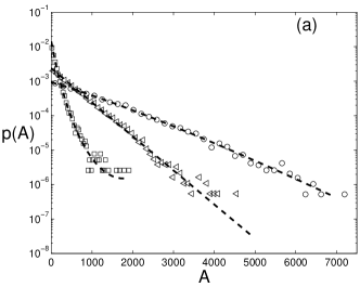
Figure 2: Numerically obtained distribution functions $p(A_{m})$ resulting from long-time integration ($t=1.1\cdot 10^{6}$) of (unstable) constant-amplitude initial states $\psi_{m}(0)=\sqrt{a}$, for a 1D DNLS chain with $N=10000$ ($C=1$). (a) $\sigma=0.4$, $a=100$ (squares), $a=455$ (triangles), and $a=1000$ (circles). (b) $\sigma=3$, $a=0.6$ (circles), and $a=0.8$ (squares). The dashed lines represent best fits to (10).

II.1.2 Standing waves

In addition to travelling waves, there are also exact solutions in the form of standing waves (SWs), which are time-periodic non-propagating (i.e., with their complex phase spatially constant) solutions, with an inhomogeneous amplitude distribution $|\psi_{m}|^{2}$ being periodic or quasiperiodic in space MJKA00 ; Morgante ; JMAK02 . In the linear limit $a\rightarrow 0$, a standing wave of wave vector $Q$ ($0<|Q|<\pi$) is a linear combination of two counterpropagating travelling waves $q=\pm Q$, i.e., $\psi_{m}\simeq\sqrt{2a}\sin(Qm+\varphi)e^{i\Lambda t}$ for small $a$. As $a$ increases, one finds MJKA00 ; Morgante ; JMAK02 , that only for particular phases $\varphi$ can these linear SWs be continued into exact nonlinear SW solutions. These can be divided into two distinct classes: phases $\varphi=\pm(\pi-Q)/2-m^{\prime}Q$ ($m^{\prime}$ integer) continue into solutions called ’type E’, while either $\varphi=-m^{\prime}Q$ (for generic $Q$) or $\varphi=-(m^{\prime}+\frac{1}{2})Q$ (for special $Q=\frac{2k+1}{2k^{\prime}+1}\pi$, $k,k^{\prime}$ integers) yield solutions called ’type H’. (These two types of solutions can be represented as elliptic and hyperbolic cycles, respectively, of the cubic real 2D map MJKA00 ; Morgante ; JMAK02 when $\sigma=1$). In physical space, they are distinguished by their positioning in the lattice, with type-E SWs centered symmetrically between lattice sites at $m=m^{\prime}+\frac{1}{2}$, and type-H SWs centered antisymmetrically either around a lattice site at $m=m^{\prime}$ (generic $Q$) or between sites at $m=m^{\prime}+\frac{1}{2}$ (for $Q=\frac{2k+1}{2k^{\prime}+1}\pi$), respectively. In the opposite limit of large $a$, which is mathematically equivalent to $C\rightarrow 0$, both classes of solutions can be generated from a circle map, distributing solutions $\psi_{m}=0,\pm\sqrt{A}e^{iA^{\sigma}t}$ periodically or quasiperiodically in space MJKA00 ; Morgante ; JMAK02 . Type-E solutions are generally linearly unstable, while type-H solutions are linearly stable for large $a/C$ but generally oscillatorily unstable for small $a/C$ (for $\sigma=1$, see Refs. MJKA00 ; Morgante ; JMAK02 ).

Particularly interesting in this context are the SWs with $Q=\pi/2$, which have the form $\psi_{2n+1}=0,\psi_{2n+2}=(-1)^{n}\sqrt{2a}e^{i(2a)^{\sigma}t}$ (type H), and $\psi_{2n+1}=\psi_{2n+2}=(-1)^{n}\sqrt{a}e^{ia^{\sigma}t}$ (type E), respectively. For small $a$, any wave (travelling or standing) with wave vector $\pi/2$ coincides with the phase transition line (9) as noted in Ref. Rumpf . This is not true in general, and in particular it is clear from (12) that a travelling wave with $q=\pi/2$ lies inside the regime of ’normal’ thermalization for all nonzero $a$. On the other hand, it was noticed in Refs. Morgante ; JMAK02 , that for $\sigma=1$ the curve $h(a)$ for the $Q=\pi/2$ type-H SW indeed coincides with the phase transition line (9), and that type-H SWs with $|Q|<\pi/2$ generally resulted in creation of large-amplitude breathers, and those with $\pi/2<|Q|<\pi$ in ’normal’ thermalization (see e.g. Figs. 6-9 in Ref. JMAK02 ). However, for general $\sigma$ we now have the relation for $Q=\pi/2$ type-H SWs:

$$h=\frac{2^{\sigma}}{\sigma+1}a^{\sigma+1}.$$ (13)

Thus, only for the particular case $\sigma=1$ considered in Refs. Morgante ; JMAK02 do the coefficients in (9) and (13) agree. In general are the transition line into the phase of statistical localization and the line defined by the $Q=\pi/2$ type-H SW different. For $0<\sigma<1$ the $\pi/2$ type-H standing wave will always be in the breather-forming regime, while for $\sigma>1$ it will always be in the normal thermalizing regime. This is illustrated by the numerical simulations in Fig. 3.

Figure 3: (a) Time-averaged (non-normalized) distribution functions $p(A_{m})$ for weakly perturbed $\pi/2$ type-H SWs with $a=1$ $(...,-\sqrt{2},0,\sqrt{2},0,...)$ as initial conditions ($C=1$). ($\ast$): $\sigma=2/3$; (+): $\sigma=1$; ($\times$): $\sigma=3$. The points are obtained by averaging over 96 time instants for $10000\leq t\leq 200000$ and $N=10000$ ($\sigma=2/3$), 177 time instants for $500000\leq t\leq 1380000$ and $N=1000$ ($\sigma=1$), and 91 time instants for $10000\leq t\leq 55000$ and $N=1000$ ($\sigma=3$). Straight lines for $\sigma=2/3$ and $\sigma=1$ are predictions from (10) with $\beta=0$ and $\gamma=1/a=1$, while curve for $\sigma=3$ is prediction from (10) with fitted values of $\beta=0.042$ and $\gamma=0.65$. (b) Average (over space and time) of the coupling part of $h$ (i.e., $<2C\sqrt{A_{m}A_{m+1}}\cos(\phi_{m}-\phi_{m+1})>$) versus time for the simulations in (a) with, from top to bottom at $t=10000$, $\sigma=2/3$, $\sigma=1$, and $\sigma=3$, respectively. Magnification in inset illustrates the slow long-time decrease for $\sigma=2/3$.

For $\sigma=3$, Fig. 3(a) clearly confirms a positive-temperature behavior, with a distribution function well fitted by (10) with positive $\beta$, and very small probability for large-amplitude excitations. For $\sigma=2/3$ we do observe, as predicted, a small positive curvature of the distribution function at finite times, as well as a tendency towards creation of large-amplitude breathers (e.g. the four points between $A=12$ and $A=14$ in Fig. 3(a)). However, even for very large systems and long integration times, the breathers found are not persistent but transient and recurring, as for the small-$\sigma$ case discussed in the previous subsection.

To check to what extent the finite-time averaged distribution functions in Fig. 3(a) are representative for the true equilibrium distributions, we monitor the average of the contribution to the total Hamiltonian from the coupling part, $h_{\rm coup}$ (first term in Eq. (2)). By definition, $<h_{\rm coup}>=0$ in equilibrium at the transition line $\beta=0$, and, by the particular choice of $\pi/2$ type-H SWs as initial conditions, $h_{\rm coup}(0)=0$ for all $\sigma$. For $\sigma=1$, Fig. 3(b) confirms that $<h_{\rm coup}>$, although being positive for intermediate times, asymptotically approaches zero as expected. For $\sigma=3$, $<h_{\rm coup}>$ approaches asymptotically a negative value, which is typical in the positive-temperature regime, and implies a preference for out-of phase excitations at neighboring sites. For $\sigma=2/3$, a superficial look at the main Fig. 3(b) seems to indicate an asymptotic approach to a strictly positive $<h_{\rm coup}>$, signifying a preference for in-phase excitations at neighboring sites. However, as is shown by the inset in Fig. 3(b), the simulation indeed has not reached a stationary regime even after $t=2\cdot 10^{5}$, and there is a very slow decrease, close to logarithmic in time, of $<h_{\rm coup}>$. We attribute this to an on-going process of formation of large-amplitude breathers. Note that, if the hypothesis of approaching a thermodynamic equilibrium state consisting of one (or a finite number of) breather(s) together with an infinite-temperature phonon bath would be correct, we should always asymptotically have $<h_{\rm coup}>=0$ in the breather-forming regime for $N\rightarrow\infty$. Thus, our simulations are consistent with (although by no means proving) this hypothesis. However, extrapolating the tendency of the curve in the inset in Fig. 3(b) to larger times would yield $<h_{\rm coup}>=0$ only after $t\sim 10^{70}$, i.e., the times to reach a true equilibrium state in the breather-forming regime are indeed extremely long! Let us only for completeness stress, that the observed slow decrease of $<h_{\rm coup}>$ is a true behavior of the system, and not an artifact of numerical drifting of the conserved quantities during the simulation time. Indeed, there is a slow numerical drift of $h$ (increasing approximately $4\cdot 10^{-12}$ per time unit), but this is negligible compared with (and in addition in the opposite direction to) the tendency in Fig. 3(b) over the used integration time.

In this context, we should also remark that, in contrast to the ordinary DNLS case $\sigma=1$ where the $Q=\pi/2$ type-H SWs are always linearly unstable for small $a$, this is not the case for $0<\sigma<1/2$ where they are linearly stable for all $a$. It follows from a standard linear stability analysis (cf. e.g. Ref. MNPS03 ), that these solutions (also termed ’period-doubled states’ in Ref. MNPS03 ) are oscillatorily unstable for small-wavelength relative perturbations when the condition $(2a)^{2\sigma}+16(1-2\sigma)<0$ is fulfilled, and linearly stable otherwise. Note that this condition is always fulfilled for small $a$ if $\sigma>1/2$, but can never be fulfilled if $\sigma<1/2$.

Regarding the type-E SW with $Q=\pi/2$, we note that this solution is a special case of the general class of equivalent solutions $\psi_{2n+1}=(-1)^{n}\sqrt{a}e^{ia^{\sigma}t},\psi_{2n+2}=(-1)^{n}\sqrt{a}e^{i\alpha_{0}}e^{ia^{\sigma}t}$, where $\alpha_{0}$ can take any real value (this class of solutions were called ’$\pi-\pi$ states’ in Ref. CP02 and ’phase states’ in Ref. MNPS03 ). Putting $\alpha_{0}=0$ yields the type-E SW with $Q=\pi/2$, while $\alpha_{0}=\pi/2$ yields the travelling wave with $q=\pi/2$. Thus, $h=a^{\sigma+1}/(\sigma+1)$ for all solutions in this class, and they belong to the ’normal’ thermalizing regime for all nonzero $a$.

II.2 Higher-dimensional models

An important point to note is, that the results from the previous subsection are readily generalized to higher-dimensional DNLS equations. Considering e.g. the 2D case for a quadratic lattice of $N$ sites, we can write the expression for the Hamiltonian analogous to (2) as

$${\mathcal{H}}=\sum_{m,n=1}^{\sqrt{N}}\left\{2C\left[\sqrt{A_{m,n}A_{m+1,n}}\cos(\phi_{m,n}-\phi_{m+1,n})+\sqrt{A_{m,n}A_{m,n+1}}\cos(\phi_{m,n}-\phi_{m,n+1})\right]+\frac{1}{\sigma+1}A_{m,n}^{\sigma+1}\right\}.$$ (14)

With this Hamiltonian, the expression for the grand-canonical partition function analogous to (5) becomes

$${\mathcal{Z}}=(2\pi)^{N}\int_{0}^{\infty}\prod_{m,n=1}^{\sqrt{N}}dA_{m,n}I_{0}(2\beta C\sqrt{A_{m,n}A_{m+1,n}})I_{0}(2\beta C\sqrt{A_{m,n}A_{m,n+1}})e^{-\beta A_{m,n}\left(\frac{A_{m,n}^{\sigma}}{\sigma+1}+\mu\right)},$$ (15)

from which we obtain the behavior close to the high-temperature limit $\beta\rightarrow 0^{+}$ again by approximating $I_{0}\approx 1$. Thus, in this limit all results are independent of dimension, which is a consequence of the equivalence of this limit to $C\rightarrow 0$, i.e., thermalized independent units which neglect all interaction terms. Thus the expression (9) for the phase-transition line is indeed valid for given $\sigma$ in any dimension!

To take a specific example in 2D, consider again a travelling plane wave $\psi_{m,n}=\sqrt{a}e^{i(q_{x}m+q_{y}n)}e^{i\Lambda t}$ (with $\Lambda=2C(\cos q_{x}+\cos q_{y})+a^{\sigma}$). It follows from standard analysis (see, e.g. Ref. Mez ), that the travelling waves are linearly stable only if $\pi/2<|q_{x}|,|q_{y}|\leq\pi$, and modulationally unstable if either $|q_{x}|$ or $|q_{y}|$ (or both) are smaller than $\pi/2$. We immediately obtain the expression for the Hamiltonian density by just replacing $\cos q$ with $\cos q_{x}+\cos q_{y}$ in the 1D expression (11), and likewise we obtain the expression for the statistical localization transition analogous to (12):

$$a^{\sigma}=\frac{2(\sigma+1)C(\cos q_{x}+\cos q_{y})}{\Gamma(\sigma+2)-1},$$ (16)

Thus, a necessary condition for breather formation from 2D travelling waves is to have $\cos q_{x}+\cos q_{y}>0$, i.e., either $|q_{x}|$ or $|q_{y}|$ (but not necessarily both) has to be smaller than $\pi/2$. Just as for 1D, the dynamics always enters the ’normal’ thermalizing regime if the norm density is large enough, and the largest possible $a$ for breather formation occurs for $q_{x}=q_{y}=0$. Note that for this constant-amplitude solution, the threshold in $a$ for $\sigma=1$ is multiplied by an additional factor of 2 compared to the analogous 1D $q=0$ case in (12), becoming $8C$ instead of $4C$.

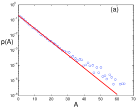
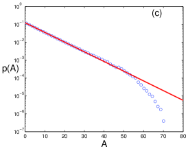
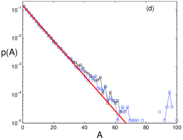
Figure 4: (Color online) Resulting distribution functions $p(A_{m})$ after long-time integrations of initial conditions consisting of weakly perturbed 2D constant-amplitude ($q_{x}=q_{y}=0$) unstable solutions with (a) $a=5$, (b) $a=7$, and (c) $a=8$. Curves in (a)-(c) have been obtained by averaging over a number of different random initial perturbations (8 in (a), 14 in (b), and 100 in (c)); system size $128\times 128$ ($N=16384$); integration times $t=500000$ (a), 200000 (b), respectively 50000 (c). Curves in (d) have been obtained from one single realization for a $50\times 50$ system with $a=7$, by averaging over 20 different time instants in the intervals $500<t<10000$ (squares), and $110000<t<300000$ (circles), respectively. The scales are such that, in (a)-(c) the dots with smallest probability correspond to one site in one realization, and in (d) to one site at one time instant. Straight lines are predictions according to (10) with $\beta=0$. ($\sigma=C=1$.)

Numerical illustrations of the resulting distribution functions in either regimes, together with predictions according to (10), are shown in Fig. 4. Note that in the breather-forming regime (Fig. 4 (a), (b), and (d)), the distributions closely follow the straight lines $p(A_{m})=\frac{1}{a}e^{-A_{m}/a}$ corresponding to $\beta=0$ in (10) up to some threshold value of $A_{m}$. We find, that extending the integration time this breaking point typically moves in the direction of larger $A_{m}$. For small integration times, one finds a smooth curve with positive curvature, indicating a negative-temperature behavior as discussed in Ref. RCKG00 . However, for larger times the tendency is that the curve becomes discontinuous, with the part below the breaking point corresponding to a phonon bath at $T=\infty$, and the points above to large-amplitude breathers with increasing amplitudes. This is illustrated by Fig. 4(d). Thus, this suggests that the separation of phase space into two parts as proposed in Ref. Rumpf is valid also for larger $a$, although, as discussed in previous subsections, the time-scales to actually reach a true equilibrium state may be enormous and beyond reach of any numerical simulations.

It should be obvious that also the extension to 3D is straightforward. We can e.g. consider a travelling plane wave in a cubic lattice, $\psi_{m_{x},m_{y},m_{z}}=\sqrt{a}e^{i(q_{x}m_{x}+q_{y}m_{y}+q_{z}m_{z})}e^{i\Lambda t}$, and obtain immediately the location of the localization transition line by adding the term $\cos q_{z}$ to the numerator of (16). Taking $\sigma=1$ and $q_{x}=q_{y}=q_{z}=0$, the critical value then becomes $a=12C$ for a constant-amplitude solution in 3D. This is illustrated numerically in Fig. 5. Again we see that the distribution (Fig. 5(a)) has the expected curvature both in the breather-forming regime (blue circles) where $\beta<0$ and in the normal regime (black circles) where $\beta>0$. In Fig. 5(b) we see that high amplitude breathers indeed do exist in the system for $a=9$.

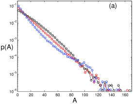
Figure 5: (Color) (a) Distribution functions $p(A_{m})$ after integrations over long but finite times ($t=5\cdot 10^{6}$) of initial conditions consisting of weakly perturbed 3D constant-amplitude ($q_{x}=q_{y}=q_{z}=0$) unstable solutions with $a=9$ (blue), $a=12$ (red) and $a=15$ (black). System size $64\times 64\times 64$ ($N=262144$), $\sigma=C=1$. (b) Intensities, in a representative $15\times 15\times 15$ subbox of the simulation box, at the end of the simulation for $a=9$ in (a). Red and yellow patches are localized breathers.

To conclude this section, we thus see that, in contrast to the condition for existence of an energy threshold for creation of a single breather, which only involves the product $\sigma D$, there is no equivalence between the spatial dimension and the degree of nonlinearity as concerns the existence of an equilibrium state with persistent breathers. Indeed, the presence or absence of such a threshold only affects the approach to equilibrium and not the qualitative features of the equilibrium state itself. The degree of nonlinearity and the dimensionality in our case actually tend to work in opposite directions, as we have seen e.g. for a constant-amplitude initial condition $\psi_{n}=\sqrt{a}$ that increasing $\sigma$ decreases the maximum amplitude $a$ for which persistent breathers form (see (12)), while increasing the dimension increases it.

III Klein-Gordon correspondence to DNLS phase transition line

Let us now discuss how the DNLS statistical localization transition manifests itself for general KG chains of coupled classical anharmonic oscillators. In order to derive approximate expressions for quantities corresponding to the DNLS Hamiltonian and norm densities valid for small amplitudes and weak coupling, we follow the perturbative approach outlined in Ref. Morgante (see also Ref. Peyrard ). The KG Hamiltonian $H$ for a chain of $N$ oscillators is given by

$$H=\sum_{n=1}^{N}\left[\frac{1}{2}\dot{u}^{2}_{n}+V(u_{n})+\frac{1}{2}C_{K}(u_{n+1}-u_{n})^{2}\right],$$ (17)

where the general on-site potential $V(u)$ for small-amplitude oscillations can be expanded as

$$V(u)=\frac{1}{2}u^{2}+\alpha\frac{u^{3}}{3}+\beta^{\prime}\frac{u^{4}}{4}+\ldots.$$ (18)

The KG equations of motion then take the form

$$\ddot{u}_{n}+V^{\prime}(u_{n})-C_{K}(u_{n+1}+u_{n-1}-2u_{n})=0.$$ (19)

Considering small-amplitude solutions $u_{n}(t)$ with typical oscillation amplitudes $|u_{n}|\sim\epsilon$, they can be formally expanded in a Fourier series as

$$u_{n}(t)=\sum_{p}a_{n}^{(p)}e^{ip\omega_{b}t},$$ (20)

where $\omega_{b}$ is close to some linear oscillation frequency and the Fourier coefficients are slowly depending on time, $a_{n}^{(p)}(\epsilon^{2}t)$. Due to exponential decay of the Fourier coefficients in $p$ they must satisfy $a_{n}^{(p)}\sim\epsilon^{p}$ for $p>0$, while $a_{n}^{(0)}\sim\epsilon^{2}$. Moreover $a_{n}^{(p)}=a_{n}^{(-p)\ast}$ since $u_{n}$ is real. Inserting (20) into (19) yields:

$$\sum_{p}\left[\ddot{a}_{n}^{(p)}+2ip\omega_{b}\dot{a}_{n}^{(p)}+(1-p^{2}\omega_{b}^{2})a_{n}^{(p)}-C_{K}(a_{n+1}^{(p)}+a_{n-1}^{(p)}-2a_{n}^{(p)})\right]e^{ip\omega_{b}t}$$

$$+\alpha\left[\sum_{p}a_{n}^{(p)}e^{ip\omega_{b}t}\right]^{2}+\beta^{\prime}\left[\sum_{p}a_{n}^{(p)}e^{ip\omega_{b}t}\right]^{3}=0+\mathcal{O}(\epsilon^{4}).$$ (21)

Then, we derive from (21) for the respective harmonics $p=0,1,2$, the three equations Morgante

$$a_{n}^{(0)}+2\alpha|a_{n}^{(1)}|^{2}-C_{K}(a_{n+1}^{(0)}+a_{n-1}^{(0)}-2a_{n}^{(0)})=0+\mathcal{O}(\epsilon^{4}),$$ (22)

$$2i\omega_{b}\dot{a}_{n}^{(1)}+\left(1-\omega_{b}^{2}\right)a_{n}^{(1)}+2\alpha(a_{n}^{(1)}a_{n}^{(0)}+a_{n}^{(1)*}a_{n}^{(2)})+3\beta^{\prime}|a_{n}^{(1)}|^{2}a_{n}^{(1)}-C_{K}(a_{n+1}^{(1)}+a_{n-1}^{(1)}-2a_{n}^{(1)})=0+\mathcal{O}(\epsilon^{5}),$$ (23)

$$(1-4\omega_{b}^{2})a_{n}^{(2)}+\alpha(a_{n}^{(1)})^{2}-C_{K}(a_{n+1}^{(2)}+a_{n-1}^{(2)}-2a_{n}^{(2)})=0+\mathcal{O}(\epsilon^{4}).$$ (24)

Consider first the case of a symmetric potential. Then, all odd powers of $u$ in the expansion (18) vanish (implying $\alpha=0$ and $\mathcal{O}(\epsilon^{5})$ in (21)), and we immediately obtain a DNLS equation to $\mathcal{O}(\epsilon^{5})$ by considering Eq. (23) for the fundamental harmonic $p=1$.

For the general (non-symmetric) case, we proceed as in Ref. Morgante by assuming weak coupling $C_{K}\sim\epsilon^{2}$ (note that this assumption is not necessary to derive the DNLS equation for the symmetric case). Then, we can solve (22) to obtain:

$$a_{n}^{(0)}=-2\alpha|a_{n}^{(1)}|^{2}+{\mathcal{O}}(\epsilon^{4}),$$ (25)

and (24) to obtain

$$a_{n}^{(2)}=\frac{\alpha}{3}(a_{n}^{(1)})^{2}+{\mathcal{O}}(\epsilon^{4}).$$ (26)

(These are the weak-coupling limits of the more general solutions (15)-(18) in Ref. Morgante .) Inserting (25)-(26) into (23), we get the general DNLS equation to $\mathcal{O}(\epsilon^{5})$

$$2i\omega_{b}\dot{a}_{n}^{(1)}+(1-\omega_{b}^{2})a_{n}^{(1)}-C_{K}(a_{n+1}^{(1)}+a_{n-1}^{(1)}-2a_{n}^{(1)})+\left(-\frac{10}{3}\alpha^{2}+3\beta^{\prime}\right)|a_{n}^{(1)}|^{2}a_{n}^{(1)}=0+\mathcal{O}(\epsilon^{5}).$$ (27)

Defining $\delta^{\prime}=\frac{\omega_{b}^{2}-1}{C_{K}}$, $\lambda^{\prime}\equiv-\frac{10}{3}\alpha^{2}+3\beta^{\prime}$, $\sigma^{\prime}\equiv sign(\lambda^{\prime})$, redefining time as $t^{\prime}=\frac{C_{K}}{2\omega_{b}}t$, rescaling the amplitudes and moving into a rotating frame by defining $\psi^{\prime}_{n}=\sqrt{{|\lambda^{\prime}|}\over C_{K}}a_{n}^{(1)}e^{i(\delta^{\prime}-2)t^{\prime}}$ and neglecting terms $\mathcal{O}(\epsilon^{5})$, the DNLS equation in the new (slow) time variable $t^{\prime}$ takes the standard form

$$i\dot{\psi}^{\prime}_{n}-(\psi^{\prime}_{n+1}+\psi^{\prime}_{n-1})+\sigma^{\prime}|\psi^{\prime}_{n}|^{2}\psi^{\prime}_{n}=0,$$ (28)

equivalent to (1) with $\sigma=1$. For (28) we have the familiar conserved quantities as norm ${\mathcal{A}}=\sum_{n=1}^{N}|\psi^{\prime}_{n}|^{2}$ and Hamiltonian ${\mathcal{H}}=\sum_{n=1}^{N}\left(\psi^{\prime\ast}_{n}\psi^{\prime}_{n+1}+\psi^{\prime}_{n}\psi^{\prime\ast}_{n+1}-\frac{\sigma^{\prime}}{2}|\psi^{\prime}_{n}|^{4}\right)$. With $h=<{\mathcal{H}}>/N$, $a=<{\mathcal{A}}>/N$ as before, the transition curve (9) between breather-forming and non-breather-forming regimes becomes $h=-\sigma^{\prime}a^{2}$ (breather-regime is above for $\sigma^{\prime}=-1$ and below for $\sigma^{\prime}=+1$.) We now wish to express this condition in KG quantities. First, we express the norm as

$${\mathcal{A}}=\frac{|\lambda^{\prime}|}{C_{K}}\sum_{n=1}^{N}|a_{n}^{(1)}|^{2}.$$ (29)

By taking $a_{n}^{(1)\ast}\cdot(\ref{DNLSgen})-a_{n}^{(1)}\cdot(\ref{DNLSgen})^{\ast}$ and summing over $n$, we find $\frac{d}{dt}\left(\sum_{n}|a_{n}^{(1)}|^{2}\right)\sim\epsilon^{6}N$, which together with (29) implies that the DNLS-norm in the general KG model behaves as ${\mathcal{A}}/N\sim\frac{\epsilon^{2}}{C_{K}}f(\epsilon^{4}t)$ (where $f$ is some function of order 1). The DNLS Hamiltonian is then expressed as

$${\mathcal{H}}=\frac{|\lambda^{\prime}|}{C_{K}^{2}}\sum_{n}\left[C_{K}(a_{n+1}^{(1)}a_{n}^{(1)\ast}+a_{n+1}^{(1)\ast}a_{n}^{(1)})-\frac{\lambda^{\prime}}{2}|a_{n}^{(1)}|^{4}\right].$$ (30)

By taking $\dot{a}_{n}^{(1)\ast}\cdot(\ref{DNLSgen})+\dot{a}_{n}^{(1)}\cdot(\ref{DNLSgen})^{\ast}$, summing over $n$ and defining ${\mathcal{H}}^{(1)}=\sum_{n}[-2\delta|a_{n}^{(1)}|^{2}+\frac{\lambda^{\prime}}{2}|a_{n}^{(1)}|^{4}+C_{K}|a_{n+1}^{(1)}-a_{n}^{(1)}|^{2}]$, where $\delta\equiv(\omega_{b}^{2}-1)/2$, we find $\frac{d{\mathcal{H}}^{(1)}}{dt}\sim\epsilon^{8}N$. Imposing the assumption of small coupling $C_{K}\sim\epsilon^{2}$ (which together with the small-amplitude condition also implies $\delta\sim\epsilon^{2}$), we get that ${\mathcal{H}}/N=-\frac{|\lambda^{\prime}|}{NC_{K}^{2}}[{\mathcal{H}}^{(1)}+2(\delta-C_{K})\sum_{n}|a_{n}^{(1)}|^{2}]\sim f(\epsilon^{4}t)$. Thus, the DNLS quantities ${\mathcal{A}}/N$ and ${\mathcal{H}}/N$ correspond in the general case to two KG quantities of order unity, whose time variation is (at least!) two orders of magnitude slower than the typical time scale for the Fourier amplitudes $a_{n}^{(1)}$ (which in turn is two orders of magnitude slower than the time scale of oscillations of the original amplitudes $u_{n}$).

Let us now explicitly calculate these quantities in terms of KG amplitudes and velocities $u_{n}$, $\dot{u}_{n}$. We do this by calculating time-averages of the different contributions to the KG Hamiltonian (17) with general potential energy (18). Inserting the expansion (20), averaging out all oscillating terms and using (25)-(26), we get

$$<\sum_{n}\frac{u_{n}^{2}}{2}>=\frac{1}{2}\sum_{n}<\left(\sum_{p=-3}^{3}a_{n}^{(p)}e^{ip\omega_{b}t}+{\mathcal{O}}(\epsilon^{4})\right)^{2}>=\sum_{n}\left(|a_{n}^{(1)}|^{2}+\frac{1}{2}(a_{n}^{(0)})^{2}+|a_{n}^{(2)}|^{2}\right)+{\mathcal{O}}(\epsilon^{6})$$

$$=\sum_{n}|a_{n}^{(1)}|^{2}+\frac{19}{9}\alpha^{2}\sum_{n}|a_{n}^{(1)}|^{4}+{\mathcal{O}}(\epsilon^{6}).$$ (31)

Further, using also (27) we get for the time-averaged kinetic energy

$$<\sum_{n}\frac{\dot{u}_{n}^{2}}{2}>=\frac{1}{2}\sum_{n}<\left(\sum_{p=-3}^{3}\left(\dot{a}_{n}^{(p)}+ip\omega_{b}a_{n}^{(p)}\right)e^{ip\omega_{b}t}+{\mathcal{O}}(\epsilon^{4})\right)^{2}>$$

$$=\omega_{b}^{2}\sum_{n}\left(|a_{n}^{(1)}|^{2}+4|a_{n}^{(2)}|^{2}\right)+i\omega_{b}\sum_{n}\left(a_{n}^{(1)}\dot{a}_{n}^{(1)\ast}-a_{n}^{(1)\ast}\dot{a}_{n}^{(1)}\right)+{\mathcal{O}}(\epsilon^{6})$$

$$=(1+2C_{K})\sum_{n}|a_{n}^{(1)}|^{2}+\left(-\frac{26}{9}\alpha^{2}+3\beta^{\prime}\right)\sum_{n}|a_{n}^{(1)}|^{4}-C_{K}\sum_{n}(a_{n+1}^{(1)}a_{n}^{(1)\ast}+a_{n+1}^{(1)\ast}a_{n}^{(1)})+{\mathcal{O}}(\epsilon^{6}).$$ (32)

For the time-averaged cubic energy we get

$$<\sum_{n}\alpha\frac{u_{n}^{3}}{3}>=\frac{\alpha}{3}\sum_{n}<\left(\sum_{p=-3}^{3}a_{n}^{(p)}e^{ip\omega_{b}t}+{\mathcal{O}}(\epsilon^{4})\right)^{3}>$$

$$=\frac{\alpha}{3}\sum_{n}\left(6a_{n}^{(0)}|a_{n}^{(1)}|^{2}+3\left(a_{n}^{(2)}(a_{n}^{(1)\ast})^{2}+a_{n}^{(2)\ast}(a_{n}^{(1)})^{2}\right)\right)+{\mathcal{O}}(\epsilon^{6})=-\frac{10}{3}\alpha^{2}\sum_{n}|a_{n}^{(1)}|^{4}+{\mathcal{O}}(\epsilon^{6}),$$ (33)

for the quartic energy

$$<\sum_{n}\beta^{\prime}\frac{u_{n}^{4}}{4}>=\frac{\beta^{\prime}}{4}\sum_{n}<\left(\sum_{p=-3}^{3}a_{n}^{(p)}e^{ip\omega_{b}t}+{\mathcal{O}}(\epsilon^{4})\right)^{4}>=\frac{3}{2}\beta^{\prime}\sum_{n}|a_{n}^{(1)}|^{4}+{\mathcal{O}}(\epsilon^{6}),$$ (34)

and for the coupling-energy

$$<\sum_{n}\frac{C_{K}}{2}(u_{n+1}-u_{n})^{2}>=2C_{K}\sum_{n}|a_{n}^{(1)}|^{2}-C_{K}\sum_{n}(a_{n+1}^{(1)}a_{n}^{(1)\ast}+a_{n+1}^{(1)\ast}a_{n}^{(1)})+{\mathcal{O}}(\epsilon^{6}).$$ (35)

Using (29), we can then write an approximate explicit expression for the DNLS norm as:

$${\mathcal{A}}=\frac{|\lambda^{\prime}|}{C_{K}}\left(<\sum_{n=1}^{N}\frac{u_{n}^{2}}{2}>+\frac{19}{30}<\sum_{n}\alpha\frac{u_{n}^{3}}{3}>\right)+{\mathcal{O}}(\epsilon^{4}).$$ (36)

Note that in particular for the symmetric case ($\alpha=0$), the DNLS norm is, to ${\mathcal{O}}(\epsilon^{4})$, directly proportional to the averaged harmonic part of the on-site potential, while for the general case there is also an additional correction due to the cubic contribution.

Then, there are several (indeed, infinitely many) ways of combining the quantities (31)-(35), which all yield approximate (to order $\epsilon^{2}$) expressions for the DNLS Hamiltonian (30). One way involving the KG Hamiltonian $H$ (17) (showing that $H$ and ${\mathcal{H}}$ indeed are nontrivially related) is to write

$${\mathcal{H}}=-\frac{|\lambda^{\prime}|}{C_{K}^{2}}\left[H-<\sum_{n}\frac{\dot{u}_{n}^{2}}{2}>-(1+2C_{K})<\sum_{n}\frac{u_{n}^{2}}{2}>-\frac{1}{2}<\sum_{n}\frac{\alpha u_{n}^{3}}{3}>\right]+{\mathcal{O}}(\epsilon^{2}).$$ (37)

This is in some sense the most appealing KG analog to the DNLS Hamiltonian, since it emphasizes the contributions from the coupling- and quartic energies to the KG Hamiltonian. Using this expression, we obtain the condition for the phase transition curve in terms of KG Hamiltonian and other quantities as:

$$\frac{H}{N}=\lambda^{\prime}\left(\frac{1}{N}<\sum_{n}\frac{u_{n}^{2}}{2}>+\frac{19}{30}\frac{1}{N}<\sum_{n}\alpha\frac{u_{n}^{3}}{3}>\right)^{2}+\frac{1}{N}<\sum_{n}\frac{\dot{u}_{n}^{2}}{2}>$$

$$+(1+2C_{K})\frac{1}{N}<\sum_{n}\frac{u_{n}^{2}}{2}>+\frac{1}{2}\frac{1}{N}<\sum_{n}\frac{\alpha u_{n}^{3}}{3}>+{\mathcal{O}}(\epsilon^{6}).$$ (38)

An example of another expression for ${\mathcal{H}}$ is

$${\mathcal{H}}=-\frac{|\lambda^{\prime}|}{2C_{K}^{2}}\left[H-2(1+2C_{K})<\sum_{n}\frac{u_{n}^{2}}{2}>-\frac{3}{2}<\sum_{n}\frac{\alpha u_{n}^{3}}{3}>-<\sum_{n}\frac{\beta^{\prime}u_{n}^{4}}{4}>\right]+{\mathcal{O}}(\epsilon^{2}),$$ (39)

which notably does not explicitly include the quartic part of the on-site energy.

Note also the following: By adding together all contributions from (31)-(35), we express the KG Hamiltonian $H$ in terms of the fundamental Fourier amplitudes $a_{n}^{(1)}$ as

$$H=2(1+2C_{K})\sum_{n}|a_{n}^{(1)}|^{2}+\left(-\frac{37}{9}\alpha^{2}+\frac{9}{2}\beta^{\prime}\right)\sum_{n}|a_{n}^{(1)}|^{4}-2C_{K}\sum_{n}\left(a_{n+1}^{(1)}a_{n}^{(1)\ast}+a_{n+1}^{(1)\ast}a_{n}^{(1)}\right)+{\mathcal{O}}(\epsilon^{6}).$$ (40)

Comparing with the expression (30) for the DNLS Hamiltonian, we see that, generally,

$$H=-\frac{2C_{K}^{2}}{|\lambda^{\prime}|}{\mathcal{H}}+2(1+2C_{K})\sum_{n}|a_{n}^{(1)}|^{2}+\left(-\frac{7}{9}\alpha^{2}+\frac{3}{2}\beta^{\prime}\right)\sum_{n}|a_{n}^{(1)}|^{4}+{\mathcal{O}}(\epsilon^{6}).$$ (41)

So in the very special case when $\alpha^{2}=\frac{27}{14}\beta^{\prime}$ the coefficient in front of $\sum_{n}|a_{n}^{(1)}|^{4}$ in (41) vanishes, and then (and only then!) is it possible to simply express the KG conserved quantity $H$ in terms of the DNLS conserved quantities ${\mathcal{H}}$ and ${\mathcal{A}}$:

$$H=\frac{2C_{K}}{|\lambda^{\prime}|}\left(-C_{K}{\mathcal{H}}+(1+2C_{K}){\mathcal{A}}\right)+{\mathcal{O}}(\epsilon^{6}),$$ (42)

and to obtain an expression for the phase transition curve involving only the average KG Hamiltonian $H/N$ and the average norm ${\mathcal{A}}/N$ (calculated e.g. using (36)):

$$\frac{H}{N}=\frac{C_{K}}{|\lambda^{\prime}|}\frac{{\mathcal{A}}}{N}\left(2C_{K}+1-C_{K}\frac{{\mathcal{A}}}{N}\right)+{\mathcal{O}}(\epsilon^{6}).$$ (43)

It is quite remarkable that one of the most studied examples, the Morse potential $V(u)=\frac{1}{2}(e^{-u}-1)^{2}$, belongs to this special class, since for Morse $\alpha=-3/2$ and $\beta^{\prime}=7/6$ ($\Rightarrow\lambda^{\prime}=-4$).

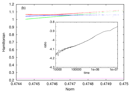
Figure 6: (color online) Numerical integration of KG Morse chain with $C_{K}=0.005$, $N=200$, and randomly perturbed constant-amplitude initial condition $u_{n}(0)=0.05$. (a) Time evolution of local energy density (note logarithmic time scale). (b) Main figure: ${\mathcal{H}}/N$ vs. ${\mathcal{A}}/N$ for the simulation in (a), with ${\mathcal{A}}$ calculated from (36) and, from top to bottom in the left part of the figure, ${\mathcal{H}}$ calculated from (39) [red], (37) [blue], and (42) [green], respectively. Time runs from right to left (i.e. ${\mathcal{A}}/N$ decreases). Lowest curve is the localization transition line (9). Inset in (b) shows the ratio of time-averaged cubic (33) to quartic (34) energies versus time, compared to the DNLS prediction (44) (lower line).

In Fig. 6 we show an example of results from long-time numerical integration of the Morse KG model, with a slightly perturbed constant-amplitude solution as initial condition. As is well-known, such an initial condition leads to breather formation through the modulational instability (e.g. Ref. Peyrard ), which is explicitly shown in Fig. 6(a). In Fig. 6(b) we show the variation of the above-derived approximate expressions for the DNLS quantities ${\mathcal{A}}$ and ${\mathcal{H}}$ during the simulation time. Note that for moderate integration times (middle part of Fig. 6(b)) the three different expressions for ${\mathcal{H}}$ are close and agree well within the expected accuracy ${\mathcal{O}}(\epsilon^{2})$. They also remain far from the localization transition line (9) (lower curve in Fig. 6(b)). However, for larger integration times the three curves diverge from each other (left part of Fig. 6(b)), where in particular (42) and (37) indicate an asymptotic decrease of ${\mathcal{H}}$ while (39) indicates an increase. This discrepancy can be traced to the fact, that the different expressions give different relative weights to the cubic and quartic anharmonic energies. As long as the amplitude remains small everywhere in the lattice, this difference is not important as all expressions are equivalent to ${\mathcal{O}}(\epsilon^{2})$. However, as breathers grow, locally the oscillation amplitudes become significantly larger, indicating the beginning of a local breakdown of the validity of the DNLS approximation at the breather sites. According to (33)-(34), the ratio between the averaged cubic and quartic parts of the anharmonic on-site energy remains fixed within the DNLS approximation,

$$<\sum_{n}\alpha\frac{u_{n}^{3}}{3}>/<\sum_{n}\beta^{\prime}\frac{u_{n}^{4}}{4}>=-\frac{20}{9}\frac{\alpha^{2}}{\beta^{\prime}}+{\mathcal{O}}(\epsilon^{2}).$$ (44)

As can be seen from the inset in Fig. 6(b), the relative contribution from the quartic energy continuously increases with time, and gets significantly larger than the DNLS prediction (44) as the breathers grow.

Figure 7: Thermalization of a quartic KG chain ($\alpha=0,\beta^{\prime}=1$) with $C_{K}=0.01$, $N=800$, coupled to a thermal bath at temperature $T^{\prime}=0.005$ with dissipation constant $\eta=0.1$. (a) Time-averaged total kinetic energy $<\sum_{n}\frac{\dot{u}_{n}^{2}}{2}>$. (b) ${\mathcal{H}}/N$ vs. ${\mathcal{A}}/N$ for the simulation in (a), with ${\mathcal{A}}$ calculated from (36), and ${\mathcal{H}}$ calculated from (37). Each dot represents a time-average over the interval $[t-100,t]$ at 15382 different times $t$. Line in (b) is the localization transition line (9). Larger points in (b) show the locations of the initial conditions used in Fig. 8.

As another illustration of the role of the DNLS quantities for the KG dynamics, we consider a thermalized KG lattice with a pure (hard) quartic potential, $V(u)=\frac{u^{4}}{4}$ (i.e., $\alpha=0$, $\beta^{\prime}=1$). We perform the following numerical experiment. First, we drive the system into a thermalized state by coupling it to a thermal bath at temperature $T^{\prime}$, using standard Langevin dynamics by adding a fluctuation term $-F_{n}(t)$ and a damping term $\eta{\dot{u}_{n}}$ to the left-hand side of (19). (Note that this temperature $T^{\prime}$ is not equivalent to the previously discussed DNLS temperature $T$, since, as shown above, the DNLS Hamiltonian ${\mathcal{H}}$ is non-trivially related to the energy $H$ of the KG-chain.) The fluctuation force $F_{n}(t)$ is taken as a Gaussian white noise with zero mean and the autocorrelation function $<F_{n}(t)F_{n^{\prime}}(t^{\prime})>=2\eta T^{\prime}\delta(t-t^{\prime})\delta_{nn^{\prime}}$, according to the fluctuation-dissipation theorem (with $k_{B}=1$). As can be seen from Fig. 7(a), with the chosen damping constant $\eta=0.1$ the lattice thermalizes after a few thousands of time units, with a time-averaged total kinetic energy $<\sum_{n}\frac{\dot{u}_{n}^{2}}{2}>=\frac{N}{2}T^{\prime}$ as expected. In the thermalized regime ($t>4000$ in Fig. 7), we monitor the quantities ${\mathcal{A}}/N$ and ${\mathcal{H}}/N$ calculated as instantaneous time-averages over fixed time-intervals ($<f(t)>=\frac{1}{t_{0}}\int_{t-t_{0}}^{t}f(t^{\prime})dt^{\prime}$, where $t_{0}=100$ in Fig. 7). The results for a large number of time instants are illustrated by the dots in Fig. 7(b). Note that taking simultaneously the limits $\beta^{\prime}T^{\prime}\rightarrow 0$ (harmonic oscillations) and $C_{K}\rightarrow 0$ (thermalized uncoupled oscillators) with $\frac{\beta^{\prime}T^{\prime}}{C_{K}}$ constant, Eqs (36) and (37) (or (39)) yield $\frac{{\mathcal{A}}}{N}\rightarrow\frac{3}{2}\frac{\beta^{\prime}T^{\prime}}{C_{K}}$ and $\frac{{\mathcal{H}}}{N}\rightarrow-\frac{9}{4}\left(\frac{\beta^{\prime}T^{\prime}}{C_{K}}\right)^{2}$, which for the parameter values of Fig. 7(b) corresponds to the point $(0.75,-0.5625)$ on the localization transition line (dashed line in the figure). As can be seen, the effect of small but nonzero coupling and anharmonicity is to shift the long-time averages (center of the ’cloud’ of dots in Fig. 7(b)) towards smaller $\frac{{\mathcal{A}}}{N}$ and larger $\frac{{\mathcal{H}}}{N}$ (approximately $(0.725,-0.505)$ in Fig. 7(b)), moving slightly into the ’non-breather-forming’ regime of the DNLS approximation. However, due to the continuous interaction with the heat bath the fluctuations are large, and the probability to be in the ’breather-forming’ regime (below the dashed line in Fig. 7(b)) at a given time-instant considerable.

Figure 8: (a) Example of a breather appearing in the microcanonical integration of an initial condition represented by the lower large point in Fig. 7 (b). (b),(c) (Non-normalized) velocity distribution functions $p(\dot{u}_{n})$ obtained from long-time numerical microcanonical integrations (points) compared to Maxwellian distributions $P(\dot{u})\sim(2\pi T^{\prime})^{-1/2}\exp(-{\dot{u}}^{2}/2T^{\prime})$ (lines) at the estimated temperature. In (b) the initial condition is the same as for (a), the temperature is $T^{\prime}\approx 0.00494$ and the integration time is $1.2\cdot 10^{6}$. (c) corresponds to the upper large point at $(0.704,-0.471)$ in Fig. 7(b), with $T^{\prime}\approx 0.00485$, and integration time $0.6\cdot 10^{6}$. In both cases, the velocities of all sites are registered in intervals of 0.6 time units. Insets in (b) and (c) show magnification of the small-velocity regime in non-logarithmic scale.

We then consider the effect of turning off the heat bath in the simulations in Fig.  7 at different time instants, and continuing a microcanonical integration with the corresponding thermalized state as initial condition. We first choose an initial condition in the ’breather-forming’ regime, corresponding to the point $(0.716,-0.568)$ in Fig.  7(b). (Even though this point is below the ’cloud’ of dots in Fig. 7(b) it does not represent a particularly exceptional initial condition in the thermal ensemble, since the dots represent time-averaged values rather than instantaneous, and the fluctuations of the latter are considerably larger.) For this particular initial condition, monitoring $<\sum_{n}\frac{\dot{u}_{n}^{2}}{2}>$ during the microcanonical integration shows that it corresponds to a lattice temperature $T^{\prime}\approx 0.00494$. It is quite remarkable, that even with integration times longer than $10^{6}$ we observe no systematic drift of either of the quantities ${\mathcal{A}}/N$ or ${\mathcal{H}}/N$. Moreover, the fluctuations of these quantities calculated as fixed-interval time-averages over 100 time units as in Fig.  7 (b) are very small (less than $5\cdot 10^{-4}$ for ${\mathcal{A}}/N$ and $3\cdot 10^{-3}$ for ${\mathcal{H}}/N$ ) and practically negligible on the scale of Fig. 7(b). Thus, the system will remain in the ’breather-forming’ regime, at least for extremely long time-scales. Although most of the breathers that can be observed are rather small and short-lived, examples of larger breathers persisting for about $20000$ time units or more are not unusual and appear repeatedly throughout the integration time (see an example in Fig. 8(a)).

To further illustrate the dynamics on the two sides of the transition line in Fig. 7(b), we compare in Fig. 8 (b), (c) the velocity distribution functions $p(\dot{u}_{n})$ obtained by long-time integration of two initial conditions corresponding to the two large points in Fig. 7(b). In the breather-forming regime (Fig. 8(b)) the calculated $p(\dot{u}_{n})$ shows a clear deviation from the standard Maxwell distribution, with a significantly enhanced probability of larger velocities ($0.2\lesssim|\dot{u}_{n}|\lesssim 0.35$ in Fig. 8(b)). Also the probability of very small velocities ($|\dot{u}_{n}|\lesssim 0.04$) is enhanced (see inset in Fig. 8(b)), while the probability for intermediate velocities is decreased compared to the Maxwell distribution (the decrease for $|\dot{u}_{n}|\gtrsim 0.35$ in Fig. 8(b) is likely to be related to the finite size of the system). Thus, the breather-forming processes tend to polarize the lattice into ’hotter’ regions of larger oscillations and ’colder’ regions of smaller oscillations, although due to the repeated creation and destruction of breathers at different sites, the equipartition result $<{\dot{u}_{n}}^{2}/2>=T^{\prime}/2$ is still valid for each site, provided that the time-average is taken over a sufficiently large interval. On the other hand, for the initial condition belonging to the ’non-breather-forming’ regime (Fig. 8(c)), no such polarization relative to the Maxwell distribution can be observed.

IV Conclusions

We have shown how a statistical-mechanics description of a general class of discrete nonlinear Schrödinger models yields explicit necessary conditions for formation of persistent localized modes, in terms of thermodynamic average values of the two conserved quantities ${\mathcal{H}}$ and ${\mathcal{A}}$. Furthermore, we illustrated how this approach can be extended to approximately describe situations with non-conserved but slowly varying quantities (see also Ref. Rumpf for a different example), and explicitly used it to explain formation of long-lived breathers from thermal equilibrium in weakly coupled Klein-Gordon oscillator chains. Concerning the roles of the degree of nonlinearity $\sigma$ and lattice dimension $D$, we found that, in contrast to the condition for existence of an energy threshold for creation of a single breather, which involves only the product $\sigma D$, $\sigma$ and $D$ tend to work in opposite directions as concerns the statistical localization transition. The energy threshold affects only the approach to equilibrium and not the qualitative features of the equilibrium state.

There are several directions in which we believe that this work should be continued. One important issue is to develop a quantitative theory determining the time-scales for approach to equilibrium in the breather-forming regime. As we have seen numerically, these time-scales may be extremely long, and naturally one may argue that the equilibrium states themselves are not physically relevant if they can only be reached after times of the order of $t\sim 10^{60}$. Another important point regards, whether the hypothesis of separation of phase space in low-amplitude ’fluctuations’ and high-amplitude ’breathers’ in the equilibrium state on the breather-forming side of the transition can be put on more rigorous grounds. Our numerical simulations are not completely conclusive in all the studied cases due to extremely long equilibration times, but give indications that this hypothesis could be valid also for large values of the norm density $a$.

Finally, we stress the important connections to current experiments: Very recently, unambiguous experimental observations of discrete modulational instabilities have been reported, for an optical nonlinear array Meier , as well as for a Bose-Einstein condensate in a moving optical lattice Fallani . It will be very interesting to see, whether such experiments also can confirm the DNLS result that the final outcome of these instabilities depend, in a qualitative and quantitative manner, on the particular values of the Hamiltonian and norm densities (the latter represents power in the optical case and particle density in the Bose-Einstein context) as predicted here.

- (1) S. Flach and C.R. Willis, Phys. Rep. 295, 181 (1998).
- (2) ”Localization and Energy Transfer in Nonlinear Systems”, edited by L. Vázquez, R. S. MacKay, and M.P. Zorzano (World Scientific, Singapore, 2003).
- (3) Yu.S. Kivshar and S. Flach, Chaos 13, 586 (2003).
- (4) D.K. Campbell, S. Flach and Yu.S. Kivshar, Phys. Today 57, 43 (2004).
- (5) R. S. MacKay and S. Aubry, Nonlinearity 7, 1623 (1994).
- (6) S. Aubry, Physica D 103, 201 (1997).
- (7) S. Aubry, G. Kopidakis, and V. Kadelburg, Disc. Cont. Dyn. Syst. -B 1, 271 (2001).
- (8) G. James, J. Nonlinear Sci. 13, 27 (2003).
- (9) G. James and P. Noble, in escorial , p. 225.
- (10) P.G. Kevrekidis, K.Ø. Rasmussen, and A.R. Bishop, Int. J. Mod. Phys. B 15, 2833 (2001).
- (11) J.C. Eilbeck and M. Johansson, in escorial , p. 44; arXiv: nlin.PS/0211049 (2002).
- (12) Yu.S. Kivshar and M. Peyrard, Phys. Rev. A 46, 3198 (1992); Yu.S. Kivshar, Phys. Lett. A 173, 172 (1993); I. Daumont, T. Dauxois, and M. Peyrard, Nonlinearity 10, 617 (1997).
- (13) A.M. Morgante, M. Johansson, G. Kopidakis, and S. Aubry, Physica D 162, 53 (2002).
- (14) K. Ø. Rasmussen, T. Cretegny, P.G. Kevrekidis, and N. Grønbech-Jensen, Phys. Rev. Lett. 84, 3740 (2000).
- (15) B. Rumpf and A.C. Newell, Phys. Rev. Lett. 87, 054102 (2001); Physica D 184, 162 (2003).
- (16) B. Rumpf, Phys. Rev. E 69, 016618 (2004).
- (17) S. Flach, K. Kladko, and R.S. MacKay, Phys. Rev. Lett. 78, 1207 (1997)
- (18) M. Weinstein, Nonlinearity 12, 673 (1999).
- (19) P.G. Kevrekidis, K.Ø. Rasmussen, and A.R. Bishop, Phys. Rev. E 61, 4652 (2000).
- (20) J. Juul Rasmussen and K. Rypdal, Phys. Scr. 33, 481 (1986).
- (21) O. Bang, J. Juul Rasmussen, and P.L. Christiansen, Nonlinearity 7, 205 (1994).
- (22) E.W. Laedke, K.H. Spatschek, and S.K. Turitsyn, Phys. Rev. Lett. 73, 1055 (1994); E.W. Laedke, O. Kluth, and K.H. Spatschek, Phys. Rev. E 54, 4299 (1996).
- (23) P.L. Christiansen, Yu.B. Gaididei, M. Johansson, K.Ø. Rasmussen, D. Usero, and L. Vázquez, Phys. Rev. B 56, 14407 (1997).
- (24) C.A. Bustamante and M.I. Molina, Phys. Rev. B 62, 15287 (2000).
- (25) M. Eleftheriou, S. Flach, and G.P. Tsironis, Physica D 186, 20 (2003).
- (26) M. Kastner, Phys. Rev. Lett. 92, 104301 (2004); arXiv:nlin.PS/0401038.
- (27) A. Smerzi and A. Trombettoni, Chaos 13, 766 (2003); Phys. Rev. A 68, 023613 (2003); C. Menotti, A. Smerzi, and A. Trombettoni, New. J. Phys. 5, 112 (2003).
- (28) M. Greiner, O. Mandel, T. Esslinger, T.W. Hänsch, and I. Bloch, Nature 415, 39 (2002).
- (29) F.S. Cataliotti, L. Fallani, F. Ferlaino, C. Fort, P. Maddaloni, and M. Inguscio, J. Opt. B: Quantum Semiclass. Opt. 5, S17 (2003); New. J. Phys. 5, 71 (2003).
- (30) M. Eleftheriou and G.P. Tsironis, arXiv:cond-mat/0308070 (2003).
- (31) M. Johansson, A.M. Morgante, S. Aubry, and G. Kopidakis, Eur. Phys. J. B 29, 279 (2002).
- (32) A.M. Morgante, M. Johansson, G. Kopidakis, and S. Aubry, Phys. Rev. Lett. 85, 550 (2000).
- (33) L. Casetti and V. Penna, J. Low Temp. Phys. 126, 455 (2002).
- (34) M. Machholm, A. Nicolin, C.J. Pethick, and H. Smith, Phys. Rev. A 69, 043604 (2004).
- (35) P.L. Christiansen, Yu.B. Gaididei, M. Johansson, K.Ø. Rasmussen, V.K. Mezentsev, and J. Juul Rasmussen, Phys. Rev. B 57, 11303 (1998).
- (36) J. Meier, G.I. Stegeman, D.N. Christodoulides, Y. Silberberg, R. Morandotti, H. Yang, G. Salamo, M. Sorel, and J.S. Aitchison, Phys. Rev. Lett. 92, 163902 (2004).
- (37) L. Fallani, L. De Sarlo, J.E. Lye, M. Modugno, R. Saers, C. Fort, and M. Inguscio, arXiv:cond-mat/0404045 (2004).