Static vortices in long Josephson junctions of exponentially varying width

Abstract

A numerical simulation is carried out for static vortices in a long Josephson junction with an exponentially varying width. At specified values of the parameters the corresponding boundary-value problem admits more than one solution. Each solution (distribution of the magnetic flux in the junction) is associated to a Sturm–Liouville problem, the smallest eigenvalue of which can be used, in a first approximation, to assess the stability of the vortex against relatively small spatiotemporal perturbations. The change in width of the junction leads to a renormalization of the magnetic flux in comparison with the case of a linear one-dimensional model. The influence of the model parameters on the stability of the states of the magnetic flux is investigated in detail, particularly that of the shape parameter. The critical curve of the junction is constructed from pieces of the critical curves for the different magnetic flux distributions having the highest critical currents for the given magnetic field.

1 Statement of the problem

A Josephson junction model that takes into account the influence of the shape in the $xy$ plane was considered in Refs. [1, 2, 3]. For a model junction with generatrices that vary by an exponential law [2, 3] (see Fig. 1) the basic equation for the phase $\varphi(t,x)$ in the junction can be written in the form

$$\ddot{\varphi}+\alpha\dot{\varphi}-\varphi\,^{\prime\prime}+\sin\varphi+g(t,x)=0\,,\quad x\in(0,l)\,,\quad t>0\,.\\$$ (1.1)

The spatial coordinate $x$ is normalized to the Josephson penetration depth $\lambda_{J}$, and $l=(L_{0}+L_{s}+L_{L})/\lambda_{J}$. The time $t$ is normalized to the plasma frequency (see, e.g., the monograph cited as Ref. [4]). The parameter $\alpha$ describes dissipative effects in the junction. An overdot denotes differentiation with respect to time $t$, and a prime denotes differentiation with respect to the spatial coordinate $x$.

The term $g(t,x)\equiv\sigma[\varphi\,^{\prime}(t,x)-h_{B}]$ in Eq. (1.1) models the current caused by the exponential variation of the width of the junction. The dimensionless shape parameter $\sigma\geq 0$ is determined by the following expression (see Fig. 1 for notation):

$$\sigma=\frac{\lambda_{J}}{L_{s}}\,\ln\left(\frac{W_{0}}{W_{l}}\right)\,,$$

where it is assumed that $W_{0}>W_{L}$. It is known that after suitable normalization the function $\varphi(t,x)$ can be interpreted as the (dimensionless) magnetic flux along the junction. Then the value of $h_{B}$ is the (dimensionless) strength of the external (boundary) magnetic field along the $y$ axis. For simplicity it is assumed below that the field $h_{B}$ is independent of time.

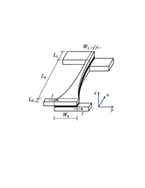
Figure 1: Diagram of the Josephson junction of exponentially varying width.

A detailed derivation of Eq. (1.1) is given in Ref. [2].

In the present paper we restrict consideration to a model junction with an in-line geometry. If the injection current density through the end $L_{0}$ of the junction is denoted by $\gamma$ (which is assumed constant), the boundary conditions at $x=0$ and $x=l$, after the transition to the corresponding limits, take the form

$$\varphi\,^{\prime}(t,0)=h_{B}-l\,\gamma,\quad\varphi\,^{\prime}(t,l)=h_{B}\,.$$ (1.2)

Because of the presence of a dissipative term $\alpha\dot{\varphi}$ the solution $\varphi(t,x)$ of equation (1.1) can lose energy and, consequently, for $t\rightarrow\infty$ it will approach the corresponding static distribution $\varphi_{s}(x)$ (to simplify the notation below we shall use the subscript $s$ when necessary). This makes it necessary to investigate in detail the static distributions in the Josephson junction and their behavior upon variations of the model parameters.

The boundary-value problem for the static distributions follows directly from relations (1.1) and (1.2):

$$-\varphi\,^{\prime\prime}+\sin\varphi+g(x)=0\,,\quad x\in(0,l)\,,$$ (1.3a)

$$\varphi\,^{\prime}\left(0\right)-h_{B}+l\gamma=0,$$ (1.3b)

$$\varphi\,^{\prime}\left(l\right)-h_{B}=0\,,$$ (1.3c)

where the “geometric” current is given by the expression

$$g(x)\equiv\sigma\left[\varphi\,^{\prime}(x)-h_{B}\right]\,.$$ (1.4)

We note that the solutions of the problem (1.3) depends not only on the spatial coordinate $x$ but also on the set of parameters $p\equiv\{l,\sigma,h_{B},\gamma\}$, i.e., $\varphi(x,p)$. When necessary below we shall indicate the dependence of the quantities on the parameters.

Let $\varphi_{s}(x)$ be some static solution of equation (1.1), i.e., a solution of the boundary-value problem (1.3). With the goal of investigating the stability of the solution $\varphi_{s}(x)$, following Ref. [5], we consider a spatiotemporal fluctuation of the form

$$\varphi(t,x)=\varphi_{s}(x)+\varepsilon\,e^{-\alpha\,t/2}\sum\limits_{n}{\left[{e^{i\omega_{n}t}\psi_{n}(x)+e^{-i\omega_{n}t}\psi_{n}^{*}(x)}\right]}\,,$$ (1.5)

which depends on the small parameter $\varepsilon$. Substituting the expansion (1.5) into Eq. (1.1) and conditions (1.2), to a first approximation in $\varepsilon$ we arrive at the Sturm–Liouville (SL) problem

$$-\psi\,^{\prime\prime}+\sigma\psi\,^{\prime}+q\,(x)\,\psi=\lambda\,\psi\,,\quad x\in(0,l)\,,$$ (1.6a)

$$\psi\,^{\prime}(0)=0,\quad\psi\,^{\prime}(l)=0\,,$$ (1.6b)

the potential of which, $q(x)\equiv\cos\varphi_{s}(x)$, is determined by the known static solution $\varphi_{s}(x)$. Here $\lambda=(\omega^{2}+\alpha^{2}/4)^{1/2}$ is the spectral parameter.

In view of the boundedness of the function $|q(x,p)|\leq 1$ on a finite interval of the variable $x$ there exists[6] a countable sequence, bounded from below, of real eigenvalues $\lambda_{\rm min}\equiv\lambda_{0}<\lambda_{1}<\lambda_{2}<\ldots<\lambda_{n}<\ldots$ of problem (1.6). To each eigenvalue $\lambda_{n}$ ($n0,1,2,\ldots)$ there corresponds a single real eigenfunction $\psi_{n}(x)$ satisfying the normalization condition

$$\int\limits_{0}^{l}{\psi^{2}_{n}(x)\,dx}=1\,.$$ (1.7)

LHere the number of zeroes of the eigenfunction $\psi_{n}(x)$ on the interval $(0,l)$ is equal to the index $n$. In particular, the eigenfunction $\psi_{0}(x)$ corresponding to the smallest eigenvalue $\lambda_{\rm min}$ does not have zeroes on $(0,l)$.

Since $\varphi(x,p)$ depends on the set of parameters $p$, the potential of the SL problem and, hence, the corresponding eigenvalues and eigenfunctions of the SL problem also depend on the parameters, i.e., $\lambda_{n}=\lambda_{n}(p)$ and $\psi_{n}=\psi_{n}(x,p)$.

We shall say [5] that in a certain range of variation of the parameters ${\cal P}\subset\mathbb{R}^{4}$ the static solution $\varphi_{s}(x)$ is stable in a first approximation with respect to spatiotemporal perturbations of the form (1.5) if in that region $\lambda_{\rm min}(p)>0$. If $\lambda_{\rm min}(p)<0$, then a component that is rapidly growing in time appears in the expansion (1.5), and the solution $\varphi_{s}(x)$ is unstable. The points of the vector of parameters which lie on the hypersurface

$$\lambda_{min}(p)=0$$ (1.8)

in the space ${\cal P}$ are points of bifurcation (branching) for the solution $\varphi(x,p)$. The values of the parameters for which Eq. (1.8) holds are called the bifurcation or critical values for the solution $\varphi(x)$. The corresponding bifurcation curves for the remaining two parameters are given by the sections of the surface (1.8) by hyperplanes corresponding to fixed values of the two parameters. The most important from the standpoint of the possibility of experimental verification are the critical curves of the current versus magnetic field type,

$$\lambda_{min}(\gamma,h_{B})=0\,,$$ (1.9)

corresponding to fixed geometric parameters $l$ and $\sigma$ of the junction.

From a theoretical standpoint knowledge of the bifurcation curves enables one to find the number of equilibrium solutions, to understand their structure, and to describe the physics of the phenomenon. Numerical simulation simplifies the study and makes it possible to estimate the range of variation of the parameters in which one can expect stability or instability of the magnetic flux distributions in the Josephson junction.

Especially important for practical purposes is the ability to check experimentally the bifurcation curves of the parameters of the Josephson junction, which in turn is an important source of information for refining the physical model. As a concrete example let us indicate the methods of studying soliton-like vortex structures of the magnetic flux in Josephson junctions on the basis of measurements of the magnetic-field dependence of the critical current (see, e.g., Refs. [3, 5] and [7, 8, 9, 10]).

We note that a number of papers have been devoted to the laying of a rigorous mathematical groundwork for reducing the problem of stability of the solutions of nonlinear operator equations to an investigation of eigenvalue problems for a linear operator (see, e.g., the review [11] and the collected papers [12] and the literature cited therein).

Josephson junctions with an exponentially varying width in the $xy$ plane have been studied theoretically and experimentally in Refs. [2] and [3]. The influence of the shape on the current–voltage characteristics of the junctions was studied in detail. However, the problems involving the determination of the stability regions of the static distributions and the structure of the critical curves have not been adequately studied. The present paper is devoted to a study of those questions, which are important from the applied and theoretical points of view.

2 Numerical results and discussion

The exact analytical solutions of equation (1.3a) for the case $\sigma=0$ are expressed in terms of elliptic functions [13]. For $\sigma>0$ approximate methods can be used [2]. In both cases a stability analysis of the solutions using the SL problem (1.6) is difficult in view of the complexity of the corresponding expressions for the potential $q(x)$. Therefore it is advisable to carry out a detailed analysis of the possible states of the magnetic flux in the junction and analysis of their stability with the help of a numerical simulation.

In this paper we use a continuous analog of Newton’s method for solution of the boundary-value problems (1.3) and (1.6), (1.7) (see reviews [14, 15]). The linearized boundary-value problems arising at each iteration were solved numerically with the use of a spline collocation scheme[16] of improved accuracy.

To permit comparison of our results with the results of Ref. [3], the majority of the numerical simulations were carried out for Josephson junctions of length $l=10$ and $l=20$.

For an “infinite” one-dimensional and uniform Josephson junction ($\sigma=0$, $l\rightarrow\infty$, $x\in(-\infty,\infty)$) the well-known exact analytical expression (see, e.g., Refs. [4] and [5])

$$\varphi(x)=4\arctan{e^{\,\pm\,x}}\,,$$ (2.1)

usually called the fluxon and antifluxon, respectively, is valid. For realistic Josephson junctions of finite length those entities are deformed by the geometry of the junction and also by the influence of the magnetic field $h_{B}$ and/or the external current $\gamma$ and are not fluxons in the strict sense of the word (the functions (2.1) do not satisfy conditions (1.2)). However, because of a number of features of those soliton-like solutions, in particular, their finite energy and size, it is appropriate and convenient to use these conventional names. For brevity below we denote the fluxon in the Josephson junction as $\Phi^{1}$.

According to [5], on the entire axis ($-\infty,\infty)$ the discrete spectrum of the SL problem generated by solution (2.1) consists of an isolated point $\lambda=0$, i.e., the fluxon/antifluxon in an “infinite” Josephson junction is found in a quasi-stable (bifurcation) state.

It follows from general comparison theorems for SL problems that for a finite Josephson junction the condition $\lambda_{\rm min}<0$ holds, i.e., the stability of $\Phi^{1}$ becomes worse.

For $\gamma=0$ and small $|h_{B}|$ the only stable state in a Josephson junction of finite length is the Meissner (vacuum) state, which will be denoted by $M$. For $h_{B}=0$, $\gamma=0$ this “trivial” solution of problem (1.3), of the form $\varphi(x)=0,\pm 2\pi,\pm 4\pi,\ldots$ (there is no magnetic field in the junction). For these same parameters the smallest eigenvalue of the SL problem for the $M$ distribution is $\lambda_{\rm min}(M)=1$. In addition to $M$ there is also an unstable Meissner solution $\varphi(x)=\pm\pi,\pm 3\pi,\ldots$, for which $\lambda_{\rm min}=-1$.

Figure 2: Fluxon vortices in a Josephson junction.

Figure 3: The $\varphi\,^{\prime}(x)$ curves for different $h_{B}$.

For sufficiently large values of the boundary magnetic field $h_{B}$, stable fluxon vortices are generated in the Josephson junction. For example, for $h_{B}=1.4$, $\gamma=0$ and $\sigma=0.07$, the Josephson junction contains, in addition to the $M$ distribution, the multifluxon vortices $\Phi^{n}$, $n=1,2,3,4$, graphs of which are shown in Fig. 3. The number of vortices is determined by the value of the total magnetic flux[5] in the Josephson junction:

$$\Delta\varphi=\varphi(l)-\varphi(0)\,.$$

For an “infinite” junction (for $l\rightarrow\infty)$ the value $\Delta\varphi/2\pi\rightarrow k$, where $k=0,2,3,\ldots$ is the number of vortices (fluxons) in the distribution $\varphi(x)$. For the solution in Fig. 3 we have, respectively, $\Delta\varphi(\Phi^{1})/2\pi\approx 1.49$, $\Delta\varphi(\Phi^{2})/2\pi\approx 2.48$, $\Delta\varphi(\Phi^{3})/2\pi\approx 3.45$, and $\Delta\varphi(\Phi^{4})/2\pi\approx 4.36$, while for the Meissner solution $\Delta\varphi(M)/2\pi\approx 0.49$.

The influence of the external magnetic field $h_{B}$ on the magnetic flux distribution $\varphi^{\prime}(x)$ in the junction for the main fluxon $\Phi^{1}$ at $\sigma=0.07$ is demonstrated in Fig. 3. At a certain value $h_{B}=h_{m}$ the maximum of the derivative $\varphi^{\prime}(x)$ is localized in the middle of the junction (curve 2, $h_{B}\approx 1.273$). For $h_{B}<h_{m}$ the fluxon is “expelled” to the end $x=l$ by the “geometric” current $g(x)$ (curve 1, $h_{B}=1$). For $h_{B}>h_{m}$ the fluxon is shifted by the external field toward the end $x=0$ (curve 2, $h_{B}=1.4)$.

If the length of the Josephson junction is sufficiently large, then a change of the current $\gamma$, equivalent to a change in magnetic field at the left end $x=0$, turns out to have only a slight influence on the local maximum magnetic field in the junction, as is well demonstrated by Fig. 5. For comparison, the situation in which the shape factor $\sigma=0$ is demonstrated in Fig. 5 for the same values of the remaining parameters. It is seen that variations of the current cause the maximum of the magnetic field to shift to the right or left of the center of the Josephson junction, depending on the direction of the current.[19]

Figure 4: The $\varphi\,^{\prime}(x)$ curve for $\sigma=0.07$.

Figure 5: The $\varphi\,^{\prime}(x)$ curve for $\sigma=0$.

For values $h_{B}>h_{m}$ the scheme $x_{m}$ of the maximum of the field $\varphi^{\prime}(x)$ of the fluxon $\Phi^{1}$ is shifted to the left from the center $x=l/2$ toward the $x=0$ end (see Fig. 3). The “motion” of the maximum of the function $\varphi^{\prime}(x)$ upon variations of the parameters of the problem occurs in accordance with the equation

$$\sin\varphi(x_{m},p)+\sigma\left[{\varphi\,^{\prime}(x_{m},p)-h_{B}}\right]=0\,,$$

which expresses the balance of the Josephson and “geometric” currents at the point $x_{m}$. Here for the $\Phi^{1}$ distribution the coordinate $x_{m}=l/2$ for $\sigma=0$, $\gamma=0$, and any attainable $h_{B}$. This case corresponds to the dashed line in Fig. 7, which shows graphs of the function $x_{m}(h_{B},\sigma)$ for several values of the shape parameter $\sigma$. Each curve for $\sigma>0$ intersects the straight line $x_{m}(h_{B},0)=l/2$ at a certain point $h_{m}(\sigma)=\varphi^{\prime}(l/2,\sigma)$ at which the maximum magnetic field inside the Josephson junction is centered. It is important to note that for $\sigma>0$ the $x_{m}(h_{B})$ curves change sharply in the vicinity of $h_{m}$: slight deviations of the external field $h_{B}$ from the value $h_{m}$ cause a significant displacement of the field maximum from the center of the junction.

Let us consider the influence of two geometric parameters of the model, viz., the shape parameter $\sigma$ and length $l$, on the magnetic flux distribution in the Josephson junction.

The dependence of the smallest eigenvalue of the SL problem for the main fluxon $\Phi^{1}$ on the shape parameter $\sigma$ is shown in Fig. 7. It is seen that for fixed $h_{B}$ and $\gamma$ there exists a certain maximum value of $\sigma$ above which the distribution of $\Phi^{1}$ loses stability, i.e., a bifurcation of the vortex occurs upon a change in $\sigma$. Large values of the magnetic field $h_{B}$ correspond to large critical values of $\sigma$. The value of the current is important at small values of $\sigma$ and plays practically no role at values of $\sigma$ close to the maximum. Figure 7 thereby demonstrates the destructive character of the shape parameter at large values of it and also the stabilizing role of the boundary magnetic field $h_{B}$.

Figure 6: “Movement” of the maximum of the magnetic field in a Josephson junction upon a change in $h_{B}$.

Figure 7: Bifurcation upon a change in $\sigma$.

The influence of the length $l$ of the Josephson junction on the stability of the main fluxon $\Phi^{1}$ is shown in Fig. 8. It is seen that $\lambda_{\rm min}(l)\approx{\rm const}$ at $l>12$, and therefore to a certain accuracy the Josephson junction can be considered “infinite” for $\Phi^{1}$. At $l<6$ the smallest eigenvalue of the SL problem (1.6) falls rapidly, going to zero at $l\approx 5.23$. Thus there exists a minimum length of the junction for which the fluxon $\Phi^{1}$ maintains stability.[18] The minimum length clearly depends on all the remaining parameters of the model — the external magnetic field $h_{B}$, the external injection current $\gamma$, and also the shape parameter $\sigma$. An analogous statement is also valid for multifluxon distributions of the magnetic flux in the junction, including unstable ones. The minimum length for multifluxon distributions $\Phi^{n}$ falls off rapidly with increasing index $n$. For example, at otherwise equal parameters the vortex $\Phi^{2}$ exists in Josephson junctions with $l>11.64$ (see Fig. 8). Consequently, if $\sigma=0.07$, $h_{B}=1$, and $\gamma=0$, then at lengths $l<5.23$ the junction is in all respects short, and the only stable distribution in the junction is the Meissner one. For $5.23<l<11.64$ the junction is short for $\Phi^{2}$, but a nontrivial stable vortex $\Phi^{1}$ can exist in it.

Figure 8: Influence of the length of the Josephson junction on thestability of $\Phi^{1}$ and $\Phi^{2}$.

Let us now consider the question of constructing by numerical means the critical current versus magnetic field relation, which is determined implicitly by Eq. (1.9) for each magnetic flux distribution in the Josephson junction. The importance of this problem stems from the possibility of measuring this relation experimentally.[3, 5, 7, 8, 9, 10] We note that for different configurations of the magnetic flux in the Josephson junction the values of the critical parameters — in particular, the critical current and magnetic field — can be substantially different. One should therefore identify the critical parameters for specific distributions and for the Josephson junction as a whole.

The curves of $\lambda_{\rm min}(h_{B})$ for the $M$ distribution and the first few stable vortices in a Josephson junction at current $\gamma=0$ and $\sigma=0$ are demonstrated in Fig. 10. For comparison the analogous curves for $\sigma=0.07$ are shown in Fig. 10. Each curve has two zeroes, the distance between which determines the stability region of the vortex upon variation of the magnetic field $h_{B}$. The zeroes themselves are critical values of the field $h_{B}$ at zero current $\gamma$.

Figure 9: The $\lambda_{\rm min}(h_{B})$ curves for $\sigma=0$.

Figure 10: The $F(h_{B})$ curves for $\sigma=0.07$.

It is well seen that the role of the shape parameter $\sigma$ is most important at small values of $h_{B}$. In particular, the $\Phi^{1}$ vortex at $\sigma=0$ exists already at $h_{B}\approx 0.054$. At $\sigma=0.07$, however, the existence region in respect to field $h_{B}$ is considerably compressed, and the vortex exists starting at $h_{B}>0.75$. The amount of compression of the $\lambda_{\rm min}(h_{B})$ curves for different vortices decreases rapidly with increasing $h_{B}$.

To complete the picture, Fig. 12 shows graphs of the total energy of several magnetic flux distributions in the Josephson junction

$$F(p)=\int\limits_{0}^{l}\left[\frac{1}{2}\,\varphi\,{{}^{\prime}\,{}^{2}}+\left(1-\cos\varphi\right)\right]\,dx-h_{B}\Delta\varphi-l\gamma\varphi(0)\,,$$ (2.2)

as a function of the external magnetic field $h_{B}$ for $\sigma=0.07$ and current $\gamma=0$. The energy values are divided by the total energy $F[\Phi^{1}]=8$ of an isolated fluxon in an infinite Josephson junction.[5] The solid and dashed curves show the energy of the stable and unstable distributions, respectively. The points of tangency of the solid and dashed curves are the points at which the magnetic flux loses stability.

Let us now consider the situation for $\gamma\neq 0$. To find the dependence of the critical current $\gamma_{c}$ on the external magnetic field $h_{B}$ it is necessary to determine the stability region with respect to current for the distributions $M$, $\Phi^{1}$, $\Phi^{2}$, etc. The results of such calculations for certain values of $h_{B}$ are given in Figs. 12 —  14.

Figure 11: The $F(h_{B})$ curves for $\sigma=0.07$.

Figure 12: The $\lambda_{\rm min}(\gamma)$ curves for $h_{B}=1.6$.

Figure 12 shows the $\lambda_{\rm min}(\gamma)$ curves for stable solutions of the problem (1.3) in a field $h_{B}=1.6$. The distances between zeroes of the functions are the stability intervals of the corresponding distributions with respect to the current $\gamma$. The right and left zeroes of the function $\lambda_{\rm min}(\gamma)$ are the positive and negative critical currents, respectively, of the distribution in the given field $h_{B}$. Because of the asymmetry of the boundary conditions (1.3b) and (1.3c) for $\gamma>0$ the critical current of the Meissner distribution [which we denote by $\gamma_{c}(M)$] is the highest, but for $\gamma<0$ the largest in modulus is the critical current $\gamma_{c}(\Phi^{1})$ of the vortex $\Phi^{1}$. Consequently, in a field $h_{B}=1.6$ the positive critical current of the junction is $\gamma_{c}=\gamma_{c}(M)$, while the negative critical current is $\gamma_{c}=\gamma_{c}(\Phi^{1})$.

We note that for the junction geometry under consideration the curve for the $M$ distribution has a characteristic plateau — the “breakoff” of the Meissner solution sets in at a rather large modulus of the external current.

Figure 13: The $\lambda_{\rm min}(\gamma)$ curves for $\Phi^{1}$.

Figure 14: The $\lambda_{\rm min}(\gamma)$ curves for $\Phi^{2}$.

Figure 14 demonstrates the $\lambda_{\rm min}(\gamma)$ curves for the main fluxon $\Phi^{1}$ at $\sigma=0.07$ and several values of $h_{B}$. The analogous curves for the $\Phi^{2}$ distribution are shown in Fig. 14. We note that with increasing external magnetic field $h_{B}$ the stability region of the vortices with respect to current is narrowed. Consequently, by varying $h_{B}$ one can construct the bifurcation curves for individual vortices to acceptable accuracy and from them determine the critical values of the current $\gamma_{c}$ for a Josephson junction.

A method of direct calculation of the bifurcation points of the vortices in a Josephson junction was proposed in Refs. [19] and [20].

Figure 16 shows the critical curves (1.8) for the main stable fluxon $\Phi^{1}$ for values of the shape parameter $\sigma=0$, $\sigma=0.001$, and $\sigma=0.07$. The solid curves correspond to a current $\gamma>0$ and the dashed curves to $\gamma<0$. We note that at a value $h_{B}\approx 1.273$ the critical curves corresponding to $\gamma>0$ intersect with each other and with the curve corresponding to $\sigma=0$ in some narrow region. This means that in that region of $h_{B}$ the critical current depends only slightly on the shape of the junction. Geometrically the influence of $\sigma$ reduces to a rotation of the critical curves clockwise about the curve for $\sigma=0$ by an angle that depends on $\sigma$. An analogous effect takes place for the critical curves corresponding to $\gamma<0$.

The critical curve $\gamma_{c}(h_{B})$ for a junction is constructed as the envelope of the critical curves corresponding to different magnetic flux distributions in the junction. In other words, the critical curve consists of pieces of the critical curves for individual states with the largest module of the critical current at a given $h_{B}$. The part of the critical curve corresponding to the interval $h_{B}\in[0,2.8)$ is illustrated in Fig. 16. For example, let $h_{B}=1.4$. At a current $\gamma=0$ there are five different magnetic field distributions in the junction, which are described above (see Fig. 3). With increasing current $\gamma$ in the direction of positive values the vortices lose stability in the following order:

$$\Phi^{4}\to\Phi^{3}\to\Phi^{2}\to\Phi^{1}\to M\,.$$

The last to break off is the Meissner distribution, the critical current of which, $\gamma_{c}(M)\approx 0.156$, is the critical current of the junction at a fixed value of the external field. Consequently, the resistive regime in the junction at $h_{B}=1.4$ exists for $\gamma>0.156$.

If the current $\gamma$ is increased from zero in the negative direction, then the breakoff of the distributions occurs in the opposite order:

$$M\rightarrow\Phi^{1}\rightarrow\Phi^{2}\rightarrow\Phi^{3}\rightarrow\Phi^{4}\,,$$

and the critical current for the junction will be that of the vortex $\Phi^{4}$: $\gamma_{c}(\Phi^{4})\approx-0.039$.

Figure 15: The critical curve of the fluxon $\Phi^{1}$.

Figure 16: The critical curve of the junction.

Analogously, for example, at $h_{B}=2.1$ the positive critical current for the junction is that of the vortex $\Phi^{5}$, $\gamma_{c}(\Phi^{5})\approx 0.034$, while the negative critical current is that of the vortex $\Phi^{6}$, $\gamma_{c}(\Phi^{6})\approx 0.024$, etc.

Of course, the “switching” of the vortices depends on all the remaining parameters of the problem. For example, for a junction with $l=10$ and $\sigma=0.07$ in an external field $h_{B}=1.6$ the order of breakoff is as follows: $\Phi^{1}\rightarrow\Phi^{2}\rightarrow M$ if $\gamma>0$, and $M\rightarrow\Phi^{2}\rightarrow\Phi^{1}$ if $\gamma<0$, as is clearly seen in Fig. 12.

We note that our numerically constructed critical curve of the Josephson junction (see Fig. 16) matches well with the theoretical and experimental results presented in Figs. 6a and 7a of [3].

3 Conclusions

We have carried out a numerical simulation of the magnetic flux distributions and their bifurcations upon variation of the model parameters in a long Josephson junction of exponentially varying width. For a stability analysis each distribution is placed in correspondence with a Sturm–Liouville problem with a potential determined by the given distribution. The distributions and, hence, the spectrum of the SL problem depend on the model parameters. It is shown that at certain critical (bifurcation) values of one or several parameters the magnetic flux in the junction can have a change of stability. For vortex configurations in a Josephson junction there are narrow regions of variation of the boundary magnetic field in which the critical current of the vortices depends only slightly on the shape parameter. Corresponding to the magnetic flux vortices are minimum lengths of the junction at which the distributions maintain their stability. The critical current versus magnetic field curves were constructed by a numerical method for the first few stable magnetic field flux distributions in a Josephson junction. The critical curve for the junction as a whole is the envelope of the critical curves of the individual distributions.

Acknowledgements

The authors thank Yu. A. Kolesnichenko (FTINT, Kharkov) for helpful discussions.

References

- [1] A. T. Filippov, T. Boyadjiev, Yu. S. Gal’pern, and I. V. Puzynin, Comm. JINR E17-89-106, Dubna (1989).
- [2] A. Benabdallah, J. G. Caputo, and A. C. Scott, Phys. Rev. B 54, 16139 (1996).
- [3] G. Carapella, N. Martucciello, and G. Costabile, cond-mat/0203055.
- [4] K. K. Licharev, Dynamics of Josephson Junctions and Circuits, Gordon and Breach, New York (1986).
- [5] Yu. S. Gal’pern and A. T. Filippov, Zh. Éksp. Teor. Fiz. 86, 1527 (1984) [Sov. Phys. JETP 59, 894 (1984)].
- [6] B. M. Levitan and I. S. Sargsyan, Sturm–Liouville and Dirac Operators [in Russian], Nauka, Moscow (1988).
- [7] Jhy-Jiun Chang and C. H. Ho, Appl. Phys. Lett. 45, 192 (1984).
- [8] A. N. Vystavkin, Yu. F. Drachevskii, V. P. Koshelets, and I. L. Serpuchenko, Fiz. Nizk. Temp. 14, 646 (1988) [Sov. J. Low Temp. Phys. 14, 357 (1988)].
- [9] B. H. Larsen, J. Mygind, and A. V. Ustinov, Phys. Lett. A 193, 359 (1994).
- [10] B. H. Larsen, J. Mygind, and A. V. Ustinov, Physica B 194–196, 1729 (1994).
- [11] M. A. Krasnosel’skiĭ, Usp. Matem. Nauk IX, vyp. 3(61), 57 (1954).
- [12] J. B. Keller and S. Antman (ed.), Bifurcation Theory and Nonlinear Eigenvalue Problems, Benjamin, Reading, Mass. (1969), Mir, Moscow (1974).
- [13] C. S. Owen and D. J. Scalapino, Phys. Rev. 164 (2), 538 (1967).
- [14] E. P. Zhidkov, G. I. Makarenko, and I. V. Puzynin, Fiz. Élem. Chastits At. Yadra 4, 127 (1973) [Sov. J. Part. Nucl. 4, 53 (1973)].
- [15] I. V. Puzynin, I. V. Amirkhanov, E. V. Zemlyanaya, V. N. Pervushin, T. P. Puzynina, T. A. Strizh, and V. D. Lakhno, Fiz. Élem. Chastits At. Yadra 30, 97 (1999) [Phys. Part. Nucl. 30, 87 (1999)].
- [16] T. L. Boyadzhiev, Soobshchenie OIYaI R2-2002-101, Dubna (2002).
- [17] T. L. Boyadzhiev, D. V. Pavlov, and I. V. Puzynin, Soobshchenie OIYaI R11-88-409, Dubna (1988).
- [18] T. L. Boyadzhiev, D. V. Pavlov, and I. V. Puzynin, in Numerical Methods and Applications, Proc. Int. Conf. Num. Math. and Appl., Bl. Sendov, R. Lazarov, and I. Dimov (eds.), Sofia, August 22–27, 1988.
- [19] D. W. McLaughlin and A. C. Scott, Phys. Rev. A 18, 1652 (1978).
- [20] T. Boyadjiev and M. Todorov, Supercond. Sci. Technology 14, 1 (2002).