Hydrodynamics for a granular gas from an exactly solvable kinetic model

Abstract

A simple exactly solvable kinetic model for the non-linear inelastic hard sphere Boltzmann equation is used to explore the relevance of hydrodynamics for a granular gas. The equation predicts a non-trivial homogeneous cooling state (HCS), including algebraic decay at large velocities. The linearized kinetic equation for small perturbations about the HCS is solved exactly. It is shown that the hydrodynamic excitations exist in this linearized dynamics, and their detailed form is shown to agree with results from the Chapman-Enskog method up through Navier-Stokes order. The existence of the hydrodynamic modes at short wavelengths, far beyond Navier-Stokes order is demonstrated as well. Finally, the precise sense in which the hydrodynamic excitations dominate the dynamics at long times is described.

1 Introduction

The applicability of a hydrodynamic description for a granular gas has been an issue of considerable interest in recent years IGoldgg ; BDMj2003 ; DBlip . The concepts involved and the precise questions to be asked have been clarified to a large extent in recent works DBlip ; BDmodes03 , and partial answers to these questions have been given. The setting for all of these discussions has been the inelastic hard sphere Boltzmann equation. However, direct demonstration of the transition to a hydrodynamic description is made difficult by the analytic complexity of the Boltzmann collision operator. The objective here is to provide such an illustration by addressing these issues in the more limited context of a simple and exactly solvable model kinetic equation for a granular gas BMD96 ; DBZ03 . This model has the primary characteristics of the Boltzmann kinetic equation: dissipation of energy, a non-trivial homogeneous cooling state (HCS), and exact macroscopic balance equations for the hydrodynamic fields. Hence it is a good starting point for a demonstration of principle in the context of granular gases.

A closed set of equations for the density, flow velocity and the granular temperature can be obtained from both the Boltzmann kinetic theory and the model kinetic theory considered here by the Chapman-Enskog procedure BDKS97 . The drawback of this procedure is its practical limitation to states with small spatial gradients, and the assumption of a special form for the solution (a ”normal” solution DBlip ). There remain questions about the space and time scales on which such a solution can be expected. Also, the lack of energy conservation has led some to question whether the local energy or temperature should properly be considered a ”slow mode” of the system that can dominate at long times.

A direct probe of these questions is possible by characterizing all the excitations in the linearized dynamics of the system for small spatial perturbations of a homogeneous state, and looking for a time scale separation between the hydrodynamic excitations and the other microscopic excitations BDmodes03 . This prescription is difficult to carry out for the hard-sphere Boltzmann equation because of the complicated collision operator involved, even at the linearized level. However, this linear problem can be solved exactly for the model under consideration here. It is found that 1) hydrodynamic excitations exist and agree with those obtained from the Chapman-Enskog method under the same conditions of long wavelengths, 2) the hydrodynamic excitations exist over a range of shorter wavelengths far beyond the restrictions of the Navier-Stokes approximation, and 3) the other dynamics (called ”microscopic” excitations) typically decay in a few collision times so that the hydrodynamic excitations dominate at long times. Some qualifications of 3) are noted. These conclusions hold even for conditions of strong dissipation.

The paper is organized as follows. First, the definition of the kinetic model is recalled and its solution for spatially homogeneous states is given. It is noted that a special HCS solution results for a wide class of initial conditions after a few collisions times. Next, weakly inhomogeneous states for small perturbations about this HCS are considered. First, the hydrodynamic description obtained from the Chapman-Enskog results is recalled in order to define ”hydrodynamic” excitations. Next, the kinetic equation is linearized and solved exactly by Fourier-Laplace transformation. The analytic properties in the complex plane determine all possible excitations, and it is shown that the hydrodynamic excitations are among these. Finally, the general solution is studied in the long wavelength limit where hydrodynamic and microscopic excitations can be displayed more explicitly. Conditions for the dominance of the hydrodynamic excitations at long times is considered in some detail. The results and remaining questions are summarized in the last section.

2 Definition of the kinetic model

A granular gas at low density is found to be well described by a system of $N$ smooth hard spheres undergoing inelastic collisions parameterized by a coefficient of restitution $\alpha$. The number density for particles with position $\mathbf{r}$ and velocity $\mathbf{v}$ at time $t$ is determined from the Boltzmann equation vNyE01 ; DuftACS01

$$\left(\frac{\partial}{\partial t}+\mathbf{v}\cdot\nabla\right)f(\mathbf{r},\mathbf{v},t)=J\left(\mathbf{r},\mathbf{v}|f(t)\right).$$ (1)

The detailed form of the collision operator $J\left(\mathbf{r},\mathbf{v}|f(t)\right)$ is not required for the purposes here, only some of its properties. Among these are its moments with respect to $1,$ $\mathbf{v}$, and $v^{2}$

$$\int d\mathbf{v}\left(\begin{array}[]{c}1\\ \mathbf{v}\\ \frac{1}{2}m\left(\mathbf{v}-\mathbf{u}\right)^{2}\end{array}\right)J\left(\mathbf{r},\mathbf{v}|f(t)\right)=\left(\begin{array}[]{c}0\\ \mathbf{0}\\ -\frac{3}{2}nT\zeta\end{array}\right).$$ (2)

Here $n$, $\mathbf{u}$, and $T$ are the local density, flow velocity, and temperature at time $t$, obtained from the distribution function according to

$$\left(\begin{array}[]{c}n(\mathbf{r},t)\\ n(\mathbf{r},t)\mathbf{u}(\mathbf{r},t)\\ \frac{3}{2}n(\mathbf{r},t)T(\mathbf{r},t)\end{array}\right)=\int d\mathbf{v}\left(\begin{array}[]{c}1\\ \mathbf{v}\\ \frac{1}{2}m\left(\mathbf{v}-\mathbf{u}\right)^{2}\end{array}\right)f(\mathbf{r},\mathbf{v,}t).$$ (3)

Finally, $\zeta$ is the ”cooling rate” (see Eq.(11) below to justify the terminology)

$$\zeta\left(\mathbf{r},t\right)=\left(1-\alpha^{2}\right)\frac{m\pi\sigma^{2}}{24n\left(\mathbf{r},t\right)T\left(\mathbf{r},t\right)}\int\,d\mathbf{v}\,\int\,d\mathbf{v}_{1}\,g^{3}\ f(\mathbf{r},\mathbf{v},t,)f(\mathbf{r},\mathbf{v}_{1},t).$$ (4)

The two zeros in Eq.(2) correspond to the conservation of mass and momentum respectively. The source in the third term implies that the energy is not conserved and the system is ”cooling” (note that it vanishes in the elastic limit of $\alpha\rightarrow 1$).   The functions $n$, $\mathbf{u}$ , and $T$ are the hydrodynamic fields, and the properties (2) together with the Boltzmann equation give the exact macroscopic balance equations relating these fields. These balance equations are the essential starting point for the formulation of a hydrodynamic description for the system. Consequently, the properties (2) should be preserved by any model kinetic theory intended to explore hydrodynamics.

The kinetic model considered here is a simple extension of the BGK model for gases with elastic collisions BGK54 , to capture the properties of a granular gas. It is obtained by replacing the bilinear collision operator in the Boltzmann equation by BMD96

$$J\left(\mathbf{r},\mathbf{v}|f(t)\right)\rightarrow-\nu\left(f-g\right),$$ (5)

where $\nu$ is a velocity independent parameter of the model and $g$ is chosen to be a functional of $f$ such that the moment conditions (2) are satisfied. As in the BGK model $g$ is taken to be a Gaussian

$$g(\mathbf{r},\mathbf{V},t\mid f)=A(\mathbf{r},t)e^{-B(\mathbf{r},t)V^{2}},$$ (6)

where $\mathbf{V}=\mathbf{v}-\mathbf{u(r,}t\mathbf{)}$ is the peculiar velocity. $A$ and $B$ are chosen so as to enforce the moment conditions above. They are found to be

$$A(\mathbf{r},t)=n(\mathbf{r},t)\left(\frac{B(\mathbf{r},t)}{\pi}\right)^{3/2},\ \ B(\mathbf{r},t)=\frac{m}{2T(\mathbf{r},t)\left(1-\frac{\zeta(\mathbf{r},t)}{\nu(\mathbf{r},t)}\right)},$$ (7)

where $m$ is the mass. In the elastic limit $g$ becomes the local Maxwellian; otherwise, the effective temperature is changed to account for the cooling implied by Eq. (2).

It remains to choose the functions $\nu(\mathbf{r},t)$ and $\zeta(\mathbf{r},t)$. In principle, these are specific functionals of $f$ in the Boltzmann equation. Here, they are taken to depend on $f$ only through the temperature and density. The cooling rate is chosen to be the same as that obtained from the Boltzmann equation by using a local Maxwellian for $f$ in Eq.(4) BMD96 . The collision frequency $\nu$ is chosen so as to fit one of the Chapman-Enskog transport coefficients of the model to that of the corresponding result from the Boltzmann equation, in this case the shear viscosity $\eta$ (for details see DBZ03 ). These choices give

$$\zeta(\mathbf{r},t)=\frac{5}{12}\left(1-\alpha^{2}\right)\nu_{0}(\mathbf{r},t),\hskip 21.68121pt\nu(\mathbf{r},t)=\left(1-\frac{1}{4}(1-\alpha)^{2}\right)\nu_{0}(\mathbf{r},t),$$ (8)

where $\nu_{0}(\mathbf{r},t)$ is an average local collision frequency

$$\nu_{0}(\mathbf{r},t)=\frac{16}{5}n(\mathbf{r},t)\sigma^{2}\sqrt{\frac{\pi T(\mathbf{r},t)}{m}}.$$ (9)

This completes the definition of the model kinetic equation

$$\left(\frac{\partial}{\partial t}+\mathbf{v}\cdot\nabla\right)f=-\nu\left(f-g\right).$$ (10)

This is deceptively simple, since the right side is a highly nonlinear functional of $f$ through its dependence on the hydrodynamics fields in $\nu$ and $g$..

3 Spatially homogeneous states

As in the case of the Boltzmann equation, there exists no spatially homogeneous steady solution to (10) for the isolated system. This can be seen by taking the second velocity moment of the kinetic equation to get

$$T^{-1}\partial_{t}T=-\zeta.$$ (11)

This implies that one of the moments of the distribution function is always time dependent and hence there is no steady solution. Instead, there is a special scaling solution, the HCS, which is approached in a few collision times by most spatially homogeneous initial conditions.

Consider a general homogeneous initial distribution and look for solutions to the model kinetic equation in the dimensionless form

$$f\left(\mathbf{v},t\right)=nv_{hcs}^{-3}f^{\ast}\left(\mathbf{v}^{\ast},s\right),\hskip 11.38092pt\mathbf{v}^{\ast}=\mathbf{v}/v_{hcs}\left(t\right)$$ (12)

Here the velocity scaling is generated by the time dependent thermal velocity and $s$ is an average collision number

$$v_{hcs}(t)=\sqrt{2T(t)/m},\hskip 21.68121ptds=\nu_{0}(t)dt.$$ (13)

The dimensionless form for the model kinetic equation becomes

$$\left(\partial_{s}+\frac{1}{2}\zeta^{\ast}\nabla_{\mathbf{v}^{\ast}}\cdot\mathbf{v}^{\ast}+\nu^{\ast}\right)f^{\ast}\left(\mathbf{v}^{\ast},s\right)=\nu^{\ast}g^{\ast}\left(\mathbf{v}^{\ast}\mid f^{\ast}\right).$$ (14)

This can be integrated directly for initial homogeneous states to get the general solution (see Appendix A and DBZ03 )

$$f^{\ast}(\mathbf{v}^{\ast},s) = e^{-\left(\frac{3}{2}\zeta^{\ast}+\nu^{\ast}\right)s}f^{\ast}(e^{-\frac{1}{2}\zeta^{\ast}s}\mathbf{v}^{\ast},0)+\nu^{\ast}\left(\pi\left(1-\frac{\zeta^{\ast}}{\nu^{\ast}}\right)\right)^{-3/2}$$ (15)

$$\times\int_{0}^{s}ds^{\prime}e^{-\left(\frac{3}{2}\zeta^{\ast}+\nu^{\ast}\right)s^{\prime}}\exp\left(-\frac{e^{-\zeta^{\ast}s^{\prime}}v^{\ast 2}}{1-\frac{\zeta^{\ast}}{\nu^{\ast}}}\right),$$

with the dimensionless constants $\nu^{\ast}=\nu/\nu_{0},$ and $\zeta^{\ast}=\zeta/\nu_{0}$. Since the state is homogeneous the flow velocity has been taken to vanish, $\mathbf{u}=0$, by making the appropriate Galilean transformation.

The constant $\nu^{\ast}$ is of order unity, so the domain of integration in (15) is exponentially bounded for $s>1$ and for large $s$ the integral becomes independent of $s$. The first term vanishes exponentially fast for initial conditions uniformly bounded in the sense $f^{\ast}(e^{-\frac{1}{2}\zeta^{\ast}s}\mathbf{v}^{\ast},0)<C$. Therefore an $s-$ independent HCS solution is obtained

$$f_{hcs}^{\ast}(v^{\ast})=\nu^{\ast}\left(\pi\left(1-\frac{\zeta^{\ast}}{\nu^{\ast}}\right)\right)^{-3/2}\int_{0}^{\infty}ds^{\prime}e^{-\left(\frac{3}{2}\zeta^{\ast}+\nu^{\ast}\right)s^{\prime}}\exp\left(-\frac{e^{-\zeta^{\ast}s^{\prime}}v^{\ast 2}}{1-\frac{\zeta^{\ast}}{\nu^{\ast}}}\right)$$ (16)

In terms of the dimensionless variables chosen, the HCS behaves as a stationary state. It is universal in the same sense as the Maxwellian for elastic collisions, since most initial homogeneous states evolve to it after a few collisions. In the following it will be chosen as the reference state to study small spatial perturbations of a homogeneous state. Clearly, the results obtained will be similar for other homogeneous reference states, but with an additional transient period as the reference state itself approaches the HCS.

4 Hydrodynamic excitations

Hydrodynamic excitations are most easily defined in the long wavelength limit where the Navier-Stokes hydrodynamic equations apply. Consider inhomogeneous states characterized by smooth spatial and temporal variations in the density, temperature and flow velocity, and for which the deviations of the hydrodynamic fields from their values in the HCS are small (linear hydrodynamics). The detailed form of these equations and the transport coefficients occurring in them have been obtained from the kinetic equation (Boltzmann and kinetic model) by the Chapman-Enskog method BMD96 ; BDKS97 and are found to be

$$\partial_{t}\delta n+n_{hcs}\nabla\cdot\delta\mathbf{u}=0,$$ (17)

$$\partial_{t}\delta u_{i}+\frac{1}{n_{hcs}m}\left(n_{hcs}\partial_{i}\delta T+T_{hcs}\partial_{i}\delta n\right)$$

$$-\frac{1}{n_{hcs}m}\left(\eta\left(\partial_{j}\delta u_{i}+\partial_{i}\delta u_{j}-\frac{2}{3}\delta_{ij}\nabla\cdot\delta\mathbf{u}\right)\right)=0,$$ (18)

$$\partial_{t}\delta T+\frac{2}{3}T_{hcs}\nabla\cdot\delta\mathbf{u}+\frac{3}{2}\zeta_{hcs}\delta T+\frac{T_{hcs}\zeta_{hcs}}{n_{hcs}}\delta n$$

$$-\frac{2}{3n_{hcs}}\left(\kappa\nabla^{2}\delta T+\mu\nabla^{2}\delta n\right)=0,$$ (19)

where $\delta x=x-x_{hcs}$ denotes the deviation of a hydrodynamic field from its value in the HCS. The transport coefficients $\eta,\kappa,$and $\mu$ occurring in the above equations have been evaluated in reference BMD96 .

The linear Navier-Stokes equations are complicated only by time dependent coefficients due to the cooling reference state. This time dependence can be eliminated by introducing the dimensionless variables, $\delta n^{\ast}=\delta n/n_{hcs}$, $\delta T^{\ast}=\delta T/T_{hcs},$ and $\delta\mathbf{u}^{\ast}=\delta\mathbf{u}/v_{hcs}$. In addition the time is transformed to the collision number $s$ in (13) and the dimensionless space variable is $\mathbf{r}^{\ast}=\mathbf{r}\nu_{0}/v_{hcs}$. Finally, since the equations are linear, it is sufficient to consider a single Fourier component

$$y_{\alpha}^{\ast}(\mathbf{r},s)=e^{i\mathbf{k\cdot r}^{\ast}}\tilde{y}_{\alpha}^{\ast}(\mathbf{k},s)$$

where the hydrodynamic fields are chosen to be

$$\tilde{y}_{\alpha}^{\ast}(\mathbf{k},s)\leftrightarrow\left(\delta n^{\ast}(\mathbf{k},s),\delta T^{\ast}(\mathbf{k},s),\delta\mathbf{u}^{\ast}(\mathbf{k},s)\cdot\widehat{\mathbf{k}},\delta\mathbf{u}^{\ast}(\mathbf{k},s)\cdot\widehat{\mathbf{e}}_{1},\delta\mathbf{u}^{\ast}(\mathbf{k},s)\cdot\widehat{\mathbf{e}}_{2}\right).$$ (20)

The components of the flow field are taken to be those along the orthonormal triplet $\{\widehat{\mathbf{k}},\widehat{\mathbf{e}}_{1},\widehat{\mathbf{e}}_{2}\}$. The dimensionless linear Navier-Stokes equations then become

$$\partial_{s}\tilde{y}_{\alpha}^{\ast}(\mathbf{k},s)+\mathcal{K}_{\alpha\beta}\tilde{y}_{\alpha}^{\ast}(\mathbf{k},s)=0,$$ (21)

with

$$\mathcal{K}=\left(\begin{array}[]{ccccc}0&0&ik&0&0\\ \zeta^{\ast}+\frac{5}{4}\mu^{\ast}k^{2}&\frac{\zeta^{\ast}}{2}+\frac{5}{4}\kappa^{\ast}k^{2}&\frac{2}{3}ik&0&0\\ i\frac{k}{2}&i\frac{k}{2}&-\frac{\zeta^{\ast}}{2}+\frac{2}{3}\eta^{\ast}k^{2}&0&0\\ 0&0&0&-\frac{\zeta^{\ast}}{2}+\frac{1}{2}\eta^{\ast}k^{2}&0\\ 0&0&0&0&-\frac{\zeta^{\ast}}{2}+\frac{1}{2}\eta^{\ast}k^{2}\end{array}\right).$$ (22)

The transport coefficients are scaled with respect to their values in the elastic limit, $\kappa^{\ast}=\kappa/\kappa_{0},$ $\eta^{\ast}=\eta/\eta_{0},$ $\mu^{\ast}=\mu n_{hcs}T_{hcs}/\kappa_{0}$, where the elastic limit values are $\kappa_{0}=15\eta_{0}/4m$ and $\eta_{0}=5(mT_{hcs})^{1/2}/16\sigma^{2}\pi^{1/2}$. The dependence of $\eta,$ $\kappa,$ and $\mu$ on the restitution coefficient $\alpha$ has been evaluated in reference BMD96 .

The initial value problem can be solved directly with the solution

$$\tilde{y}^{*}_{\alpha}(\mathbf{k},s)=\sum_{\beta}C_{\alpha\beta}e^{z_{\beta}(k)s}.$$ (23)

Here $C_{\alpha\beta}$ are constants and $z_{\beta}(k)$ are the eigenvalues of $\mathcal{K}\left(k\right)$ determined from

$$\det\left(z(k)\mathbf{1+}\mathcal{K}(k)\right)=0.$$ (24)

As the Navier-Stokes equations are valid only up through order $k^{2}$ the solutions to this equation are relevant only to the same order

$$z_{\alpha}(k) \rightarrow \left\{-\frac{1}{\zeta^{\ast}}k^{2},-\frac{\zeta^{\ast}}{2}+\left(\frac{2}{3\zeta^{\ast}}-\frac{5}{4}\kappa^{\ast}\right)k^{2},\frac{\zeta^{\ast}}{2}-\left(\frac{1}{3\zeta^{\ast}}+\frac{2}{3}\eta^{\ast}\right)k^{2},\right.$$ (25)

$$\left.\frac{\zeta^{\ast}}{2}-\frac{1}{2}\eta^{\ast}k^{2},\frac{\zeta^{\ast}}{2}-\frac{1}{2}\eta^{\ast}k^{2}\right\}.$$

For the discussion below it is noted that in particular, at $k=0$, these become

$$z_{\alpha}(0)\rightarrow\left\{0,-\frac{\zeta^{\ast}}{2},\frac{\zeta^{\ast}}{2},\frac{\zeta^{\ast}}{2},\frac{\zeta^{\ast}}{2}\right\}.$$ (26)

The hydrodynamic excitations can now be defined precisely. They are the excitations of the form (23) with $z_{\beta}(k)$ defined to be the frequencies that are continuously connected to $z_{\alpha}(0)$ defined in (26) as $k$ goes to zero. When such modes can be identified it is said that hydrodynamic excitations exist. In that case, an internal consistency check is the agreement of those modes with the Chapman-Enskog results (25) at order $k^{2}$. The modes $z_{4}(k)=z_{5}(k)$ are associated with the components of the flow field orthogonal to the $\mathbf{k}$. These are called transverse shear modes. The other three modes are called longitudinal modes. Since $\mathcal{K}$ is block diagonal the transverse modes decouple from the other modes and hence can be treated more easily and directly.

5 Linear kinetic theory

In the rest of the paper, the dimensionless variables introduced in the previous sections are used throughout and the asterisk is deleted for simplicity of notation. To describe small perturbations of the distribution function about the HCS solution, define $\delta f$ by

$$f=f_{hcs}+\delta f.$$ (27)

Substitution of this form into the kinetic equation (10) and retaining only linear order terms in $\delta f$ defines the linear kinetic theory. The model collision operator of (10) depends on the distribution function explicitly and implicitly through the hydrodynamic fields in $\nu$ and $g$. The linearized kinetic equation is identified in Appendix B and is found to be

$$\left(\partial_{s}+\mathbf{v}\cdot\nabla_{\mathbf{r}}+\nu+\frac{1}{2}\zeta\nabla_{\mathbf{v}}\cdot\mathbf{v}\right)\delta f=M_{\alpha}y_{\alpha}$$ (28)

where

$$M_{a}(\mathbf{v})=\left(\begin{array}[]{c}\left(\zeta\nabla_{\mathbf{v}}\cdot\mathbf{v}+\nu\right)f_{hcs}\\ \frac{1}{2}\nabla_{\mathbf{v}}\cdot\mathbf{v}\left(\frac{1}{2}\zeta-\left(\frac{1}{2}\zeta\nabla_{\mathbf{v}}\cdot\mathbf{v}+\nu\right)\right)f_{hcs}\\ \left(-\frac{1}{2}\zeta-\left(\frac{1}{2}\zeta\nabla_{\mathbf{v}}\cdot\mathbf{v}+\nu\right)\right)\nabla_{\mathbf{v}}f_{hcs}\end{array}\right).$$ (29)

The hydrodynamic fields $y_{\alpha}$ are defined in (20). The kinetic equation can be solved by a Fourier-Laplace transformation

$$\delta\tilde{\tilde{f}}(\mathbf{k},\mathbf{v},z)=\int_{0}^{\infty}dse^{-zs}\int d\mathbf{r}e^{i\mathbf{k\cdot r}}\delta f(\mathbf{r},\mathbf{v},s).$$ (30)

The formal solution is

$$\delta\tilde{\tilde{f}}(\mathbf{k},\mathbf{v},z)=\mathcal{R}\delta\tilde{f}(\mathbf{k},\mathbf{v},0)+\tilde{\tilde{y}}_{\alpha}(\mathbf{k},z)\mathcal{R}M_{\alpha}(\mathbf{v})$$ (31)

where the resolvent operator $\mathcal{R}$ is

$$\mathcal{R}(\mathbf{k},z)=\left(z+\nu+i\mathbf{k}\cdot\mathbf{v}+\frac{1}{2}\zeta\nabla_{\mathbf{v}}\cdot\mathbf{v}\right)^{-1}$$ (32)

This is an implicit solution for $\delta\tilde{f}(\mathbf{k},\mathbf{v},z)$ because the hydrodynamic fields $\left\{\tilde{\tilde{y}}_{\alpha}\right\}$ are linear functionals of $\delta\tilde{\tilde{f}}$

$$\tilde{\tilde{y}}_{\alpha}(\mathbf{k},z)=\int d\mathbf{v}\phi_{\alpha}\left(\mathbf{v}\right)\delta\tilde{\tilde{f}}(\mathbf{k},\mathbf{v},z).$$ (33)

where

$$\phi_{\alpha}=\left(1,\left(\frac{2}{3}v^{2}-1\right),\mathbf{v}\cdot\widehat{\mathbf{k}},\mathbf{v}\cdot\widehat{\mathbf{e}}_{1},\mathbf{v}\cdot\widehat{\mathbf{e}}_{2}\right)$$ (34)

The $\left\{\tilde{\tilde{y}}_{\alpha}\right\}$ can be determined self-consistently using (31) in (33) to get

$$\tilde{\tilde{y}}_{\alpha}(\mathbf{k},z)=(\mathbf{1}-Q(\mathbf{k},z))_{\alpha\beta}^{-1}I_{\beta}(\mathbf{k},z)$$ (35)

where

$$I_{\alpha}=\int d\mathbf{v}\phi_{\alpha}(\mathbf{v})\mathcal{R}\delta\tilde{f}(\mathbf{k},\mathbf{v},0),\hskip 11.38092ptQ_{\alpha\beta}=\int d\mathbf{v}\phi_{\alpha}(\mathbf{v})\mathcal{R}M_{\beta}.$$ (36)

Finally, substitution of (35) in (31) gives the desired solution

$$\delta\tilde{\tilde{f}}(\mathbf{k},\mathbf{v},z)=\mathcal{R}\delta\tilde{f}(\mathbf{k},\mathbf{v},0)+\mathcal{R}M_{\alpha}(\mathbf{v})(\mathbf{1}-Q)_{\alpha\beta}^{-1}I_{\beta}(\mathbf{k},z).$$ (37)

It remains to make explicit the action of the resolvent operator in (37). This is determined in Appendix A with the result, for an arbitrary function of the velocity $X\left(\mathbf{v}\right)$,

$$\mathcal{R}X\left(\mathbf{v}\right)=\int_{0}^{\infty}dse^{-\left(z+\nu+\frac{3}{2}\zeta\right)s}\exp\left(\frac{2}{\zeta}\left(e^{-\frac{1}{2}\zeta s}-1\right)i\mathbf{k}\cdot\mathbf{v}\right)X\left(e^{-\frac{1}{2}\zeta s}\mathbf{v}\right),$$ (38)

In this way the general linear solution (37) is reduced to quadratures. $I$ and $Q$ in Eq.(36) are evaluated in Appendix C.

5.1 Transverse modes

The analysis for transverse shear mode excitations is simplest and illustrates the more general case. Consider an initial perturbation in the transverse flow velocity only

$$\delta\tilde{f}(\mathbf{k},\mathbf{v},0)=-\widehat{\mathbf{e}}_{1}\cdot\nabla_{\mathbf{v}}f_{hcs}\left(v\right)\delta\tilde{u}_{t}(\mathbf{k},0)\hskip 21.68121ptu_{t}=\mathbf{u\cdot}\widehat{\mathbf{e}}_{1}$$ (39)

This perturbation results from a small change in the velocity of the HCS along the transverse direction $\widehat{\mathbf{e}}_{1}$. It couples only to $\mathbf{u\cdot}\widehat{\mathbf{e}}_{1}$ (due to symmetry) and Eq. (35) for the response of that field reduces to

$$\delta\tilde{\tilde{u}}_{t}(\mathbf{k},z)=\frac{I(\mathbf{k},z)}{1-Q_{44}(\mathbf{k},z)}\delta\tilde{u}_{t}(\mathbf{k},0).$$ (40)

with $I(\mathbf{k},z)=I_{4}(\mathbf{k},z)/\delta\tilde{u}_{t}(\mathbf{k},0)$. The functions $I(\mathbf{k},z)$and $Q_{44}(\mathbf{k},z)$ are evaluated using the property ( 38) with the results

$$I(k,z)=\int_{0}^{\infty}dse^{-\left(z+\nu-\frac{1}{2}\zeta\right)s}\nu\int_{0}^{\infty}ds^{\prime}e^{-\nu s^{\prime}}\allowbreak\exp\left(-e^{\zeta s^{\prime}}a(s)k^{2}\right),$$ (41)

where

$$a(s)=\left(1-\frac{\zeta}{\nu}\right)\left(\frac{e^{\frac{1}{2}\zeta s}-1}{\zeta}\right)^{2}.$$ (42)

Similarly, $Q_{44}(k,z)$is found to be

$$Q_{44}(k,z)=\left(\nu-\zeta k^{2}\frac{d}{dk^{2}}\right)\tilde{\tilde{I}}(k,z)$$ (43)

Consider first the long wavelength limit $k\rightarrow 0$

$$I(\mathbf{0},z)=\frac{1}{z+\nu-\frac{\zeta}{2}},\hskip 21.68121pt1-Q(\mathbf{0},z)=\frac{z-\frac{\zeta}{2}}{z+\nu-\frac{\zeta}{2}}\hskip 21.68121pt$$ (44)

$$\delta\tilde{\tilde{u}}_{t}(\mathbf{k},z)\rightarrow\frac{1}{z-\frac{1}{2}\zeta}\delta\tilde{u}_{t}(\mathbf{k},0).$$ (45)

Comparison with (26) shows that this is the expected hydrodynamic pole, confirming the existence of hydrodynamics in the kinetic theory for response to a transverse perturbation.

The hydrodynamic pole in the long wavelength limit arises from the zero of $1-Q_{44}(\mathbf{0},z(0)).$ Its continuation to $z(k)$ at finite $k$ is therefore defined to be the solution to

$$1-Q_{44}(\mathbf{k},z(k))=0,\hskip 21.68121pt$$ (46)

with the condition $z(0)=\zeta/2$ (the poles of the function $\tilde{\tilde{I}}(\mathbf{k},z)$ determine the microscopic excitations in $\delta\tilde{\tilde{u}}_{t}(\mathbf{k},z)$ for finite $k$). It is easily shown that $z(k)$ is a real function of $k^{2}$. The integrals above are defined only for $z>\frac{\zeta}{2}-\nu.$ Therefore, the hydrodynamic pole can exist only for values of $k$ such that $z\left(k\right)>-\left(\nu-\frac{\zeta}{2}\right).$

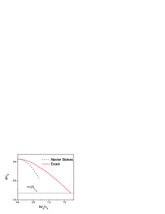
Figure 1: Transverse hydrodynamic mode

Figure 1 illustrates the numerical solution to (46) for $\alpha=0.8$, showing the hydrodynamic pole exists for all $k<k_{m}$, where $z\left(k_{m}\right)=\frac{\zeta}{2}-\nu$. For small $k$ direct expansion of (46) to order $k^{2}$ gives the solution

$$z(k)\rightarrow\frac{1}{2}\zeta(\alpha)-\frac{1}{2}\eta(\alpha)k^{2}.$$ (47)

This is the same form as that for the transverse hydrodynamic mode obtained from the Navier-Stokes equation in (25). The shear viscosity obtained here is

$$\eta(\alpha)=\frac{1}{\left(\nu(\alpha)-\frac{1}{2}\zeta(\alpha)\right)},$$ (48)

which is the same as that found by the Chapman-Enskog method in BMD96 and hence is an independent verification of that method. Interestingly, Figure 1 suggests that the Navier-Stokes approximation begins to fail for relatively small wavevectors.

5.2 Longitudinal modes

Return now to the general solution (31) and consider initial conditions that generate the perturbations $\delta\tilde{n}(\mathbf{k},0),$ $\delta\tilde{T}(\mathbf{k},0),$ and $\delta\tilde{\mathbf{u}}(\mathbf{k},0)\cdot\widehat{\mathbf{k}}$. The Laplace transform of these fields at later times is given by (35)

$$\tilde{\tilde{y}}_{\alpha}(\mathbf{k},z)=(\mathbf{1}-Q(\mathbf{k},z))_{\alpha\beta}^{-1}I_{\beta}(\mathbf{k},z),\hskip 21.68121pt\alpha,\beta=1,2,3.$$ (49)

The integrals $I_{\beta}(\mathbf{k},z)$and $Q_{\alpha\beta}(\mathbf{k},z)$ can be calculated exactly just as for the transverse perturbation above. As in that case, the poles of $(\mathbf{1}-Q(\mathbf{k},z))^{-1}$gives the hydrodynamic excitations. In place of (46), the longitudinal hydrodynamic modes are now defined by the three solutions to

$$\det(\mathbf{1}-Q(\mathbf{k},z\left(k\right)))=0.$$ (50)

At $k=0$, the matrix $\mathbf{1}-Q(\mathbf{k},z)$ is found to be

$$\mathbf{1}-Q(\mathbf{0},z)=\left(\begin{array}[]{ccc}\frac{z}{z+\nu}&0&0\\ -\frac{\nu-2\zeta}{z+\nu-\zeta}+\frac{\nu}{z+\nu}&\frac{z+\frac{\zeta}{2}}{z+\nu-\zeta}&0\\ 0&0&\frac{z-\frac{\zeta}{2}}{z+\nu-\frac{\zeta}{2}}\end{array}\right).$$ (51)

The solutions to (50) give the longitudinal modes in the long wavelength limit

$$z(0)\rightarrow\left\{0,-\frac{\zeta}{2},\frac{\zeta}{2}\right\}.$$ (52)

Comparison with (26) shows that these are indeed the hydrodynamic modes.

It is straight forward to extend the calculation of these modes by expanding $Q(\mathbf{k},z)$ to order $k^{2}$. The solutions to (50) are found to be the same as in (25)

$$z(\mathbf{k})\rightarrow\left\{0+\frac{1}{\zeta}k^{2},-\frac{\zeta}{2}+\left(\frac{2}{3\zeta}-\frac{5}{4}\kappa\right)k^{2},\frac{\zeta}{2}-\left(\frac{1}{3\zeta}+\frac{2}{3}\eta\right)k^{2}\right\}.$$ (53)

The shear viscosity $\eta$ is again given by (48), while the thermal conductivity $\kappa$ is

$$\kappa(\alpha)=\frac{2((\nu(\alpha)-\zeta(\alpha))^{2}+\zeta^{2}(\alpha))}{3(\nu(\alpha)-2\zeta(\alpha))^{2}\nu(\alpha)}.$$ (54)

This agrees in detail with the expression obtained by the Chapman-Enskog procedure BMD96 .

The results of this section complete the first objective of this work: demonstration that the hydrodynamic excitations exist in the solution to the linear kinetic equation for small perturbations of the HCS. The form of the hydrodynamic modes to Navier-Stokes order and dependence of the transport coefficients on the restitution coefficient is confirmed in detail, providing independent support for the assumptions of the Chapman-Enskog method. In addition, Figure 1 shows that the hydrodynamic modes exist far beyond the validity domain for the Navier-Stokes approximation. For the example considered here that domain appears to be quite restricted.

6 Approach to hydrodynamics

The second objective of this work is to verify that the hydrodynamic excitations are the slowest modes at long wavelengths and therefore dominate at long times. First, the general solution to the linearized kinetic equation (37) is reconsidered to display all of the possible excitations.

$$\delta\tilde{\tilde{f}}(\mathbf{k},\mathbf{v},z)=\mathcal{R}\delta\tilde{f}(\mathbf{k},\mathbf{v},0)+\mathcal{R}M_{\alpha}(\mathbf{v})(\mathbf{1}-Q(\mathbf{k},z))_{\alpha\beta}^{-1}I_{\beta}(\mathbf{k},z).$$ (55)

The dynamics arises from two types of contributions. The first is the non-hydrodynamic behavior generated by the resolvent operator in $\mathcal{R}\delta\tilde{f}$, $\mathcal{R}M_{\alpha}$, and $I_{\beta}(\mathbf{k},z)$ (see Eq. (38)). The hydrodynamic exciations arise from the simple poles of $(\mathbf{1}-Q(\mathbf{k},z))_{\alpha\beta}^{-1}$. Also, there is a convolution of the hydrodynamic and non-hydrodynamic behavior. All of these effects are present even for $k\rightarrow 0$, where these expressions can be made more explicit. Hence the following analysis is first carried out at $k=0$ and then it is argued that the conclusions extend to $k\neq 0$ by continuity.

Using (38) and the results of the previous section at $k=0$ the general solution can be written exactly

$$\delta\tilde{f}(\mathbf{0},\mathbf{v},s) = \sum_{\alpha}e^{z_{\alpha}(0)s}\chi_{\alpha}(\mathbf{v})\tilde{y}_{\alpha}^{\prime}(\mathbf{0},0)+e^{-\left(\frac{3}{2}\zeta+\nu\right)s}\left(\delta\tilde{f}(\mathbf{0},e^{-\frac{1}{2}\zeta s}\mathbf{v},0)\right.$$ (56)

$$\left.+\sum_{\alpha}e^{z_{\alpha}(0)s}\chi_{\alpha}(e^{-\frac{1}{2}\zeta s}\mathbf{v})y_{\alpha}^{\prime}(0)\right),$$

The new hydrodynamic fields $\left\{y_{\alpha}^{\prime}\right\}$in (56) are linear combinations of $\left\{y_{\alpha}\right\}$and the functions $\chi_{\alpha}\left(\mathbf{v}\right)$are the corresponding linear combinations of $M_{\alpha}(\mathbf{v})$

$$y_{\alpha}^{\prime}=\left\{\delta n,\delta n+\frac{\delta T}{2},\delta\mathbf{u}\right\},\hskip 7.22743pt\chi_{\alpha}=\left\{\left(f_{hcs}+\nabla_{\mathbf{v}}\cdot\mathbf{v}f_{hcs}\right),-\nabla_{\mathbf{v}}\cdot\mathbf{v}f_{hcs},\nabla_{\mathbf{v}}f_{hcs}\right\}.$$ (57)

The first term on the right side of (56)is the contribution from hydrodynamic excitations. It could have been constructed directly from the solution to the linearized kinetic equation as an eigenvalue problem. Then $\chi_{\alpha}(\mathbf{v})$ would be the hydrodynamic eigenfunctions. This has been done in BDmodes03 and the above $\chi_{\alpha}$ are indeed the eigenfunctions found there.

All other excitations in the system are contained in the second term of (56). Nominally, this appears to decay as $\exp(-\left(\frac{3}{2}\zeta+\nu\right)s)$. This is misleading, however, due to the additional time dependence in the functions of velocity. Consider first the moments giving the hydrodynamic fields $y_{\alpha}^{\prime}(\mathbf{k},s)$

$$y_{\alpha}^{\prime}(\mathbf{k},s)=\int d\mathbf{v}\psi_{\alpha}(\mathbf{v})\delta\tilde{f}(\mathbf{k},\mathbf{v},s),\hskip 21.68121pt\psi_{\alpha}=\left\{1,\frac{1}{3}v^{2}+\frac{1}{2},\mathbf{v}\right\}.$$ (58)

Then (56) gives

$$y_{\alpha}^{\prime}(\mathbf{0},s) = e^{z_{\alpha}(0)s}\tilde{y}_{\alpha}^{\prime}(\mathbf{0},0)+e^{-\nu s}\int d\mathbf{v}\psi_{\alpha}\left(e^{\frac{1}{2}\zeta s}\mathbf{v}\right)\left(\delta\tilde{f}(\mathbf{0},\mathbf{v},0)\right.$$ (59)

$$\left.+\sum_{\alpha}e^{z_{\beta}(0)s}\chi_{\beta}(\mathbf{v})y_{\beta}^{\prime}(\mathbf{0},0)\right)$$

Since the functions $\psi_{\alpha}\left(\mathbf{v}\right)$ are polynomials of maximum degree $2$, the second term decays as $\exp(-\left(\nu-\zeta\right)s)$. The fastest decaying hydrodynamic mode is that with $z_{2}(0)=-\zeta/2$. Thus the hydrodynamic modes are bounded away from all of the microscopic modes and the fields $y_{\alpha}^{\prime}(\mathbf{0},s)$ obey the hydrodynamic equations for long times, if $\nu>3\zeta/2$. This must be the case since this condition characterizes energy loss, according to the moment conditions on the collision integral (2). For the model considered, $3\zeta/2=$$5\left(1-\alpha^{2}\right)/8$ and $\nu=1-(1-\alpha)^{2}/4$, so the condition holds even at $\alpha=0$.

Now consider other properties obtained as averages over the distribution function. In general, for a property determined from $A(\mathbf{v})$

$$\left\langle A;s\right\rangle = \left\langle A(\mathbf{v})\right\rangle_{hcs}+\sum_{\alpha}e^{z_{\alpha}(0)s}y_{\alpha}^{\prime}(0)\int d\mathbf{v}A(\mathbf{v})\chi_{\alpha}(\mathbf{v})$$ (60)

$$+e^{-\nu s}\int d\mathbf{v}A(e^{\frac{1}{2}\zeta s}\mathbf{v})\left(\delta\tilde{f}(\mathbf{0},\mathbf{v},0)+\sum_{\alpha}e^{z_{\alpha}(0)s}\chi_{\alpha}(\mathbf{v})y_{\alpha}^{\prime}(0)\right)$$

For any bounded function $\left|A(\mathbf{v})\right|<G$ the last term decays as $e^{-\nu s}$, and since $\nu>\zeta/2$ the hydrodynamic contribution dominates for long enough times. However, a peculiarity occurs for unbounded functions of sufficiently high degree. Suppose $A(\mathbf{v})\sim v^{p}$ for large $\mathbf{v}$. Then the last integral will have a contribution behaving as $\exp(-\left(\nu-\frac{p}{2}\zeta\right)s)$. The maximum value of $p$ is restricted by the condition that the average in the reference state, $\left\langle A(\mathbf{v})\right\rangle_{hcs}$, should be finite. This condition gives $p<2\nu/\zeta$, so the exponent for the second term remains negative. Nevertheless, the decay rate can be made as small as desired within this restriction. In particular, it can be chosen to give a decay that is slower than the fastest hydrodynamic modes at $\zeta/2$. For such properties, the hydrodynamic excitations contribute but they do not dominate at long times.

The conclusion of this last paragraph suggests new limitations on hydrodynamics for granular gases. There are two ways to avoid such a conclusion. The first is to assume that such properties that behave as $A(\mathbf{v})\sim v^{p}$ with $\left(\nu-\frac{p}{2}\zeta\right)<\zeta/2$ are unphysical or uninteresting. For example, at $\alpha=0.9$ this gives $p>11$. A more precise avoidance of the problem is to formulate the linear kinetic theory problem in an appropriate Hilbert space whose scalar product is defined by

$$\left(a,b\right)=\int d\mathbf{v}f_{hcs}\left(\mathbf{v}\right)a^{\ast}\left(\mathbf{v}\right)b\left(\mathbf{v}\right).$$

The solutions of interest are then $\delta f=f_{hcs}\mathbf{\Delta}$, where $\Delta$ must lie in the Hilbert space. Similarly, the properties whose averages are considered must also be in that Hilbert space. Then square integrability changes the above restriction on $p$ to $2p<2\nu/\zeta$. This restores the dominance of hydrodynamics at long times for all admissible physical properties. The choice of a Hilbert space may seem artificial since normalization of the distribution function requires only existence in $L_{1}$. However, for normal gases the Hilbert space has been justified on the basis of the existence of the H functional, or entropy, when linearized about the equilibrium state. Perhaps there is a corresponding functional for granular gases leading to the same conclusion.

7 Summary and conclusions

Granular gases are significantly different from normal gases. Energy is not conserved. So, the homogeneous states for an isolated system are time dependent and the velocity distribution is not Maxwellian. Such states are unstable with respect to small spatial perturbations. These peculiarities have often been cited as reasons to question the relevance of hydrodynamics for granular gases, or at least to expect severe limitations on the applicability of such a description. The model kinetic equation considered here supports all of these peculiarities and therefore provides a good testing ground for such concerns. Previously, the model has been used to derive hydrodynamic equations by the Chapman-Enskog method for states with small spatial gradients. The analysis here is complementary, in the sense that it leads to the same results under those restricted conditions but describes as well the case of large gradients and the time scale leading up to the hydrodynamic stage.

The problem posed here is to solve exactly the linear kinetic equation for small spatial perturbations of the homogeneous reference state (HCS). This has been accomplished by first solving the equation for the HCS and then constructing a solution to the linear equation valid for arbitrary space and time scales. It has been shown that hydrodynamic excitations exist in this general solution by identifying them explicitly at long wavelengths and assuming an analytic connection to shorter wavelengths. In this way the Navier-Stokes hydrodynamic excitations are demonstrated explicitly. The existence of hydrodynamic excitations at shorter wavelengths was illustrated for the special case of the shear mode. In the last section above, it has been shown that these excitations dominate the other dynamics for the hydrodynamic fields and other average properties after a few collisions. In summary, it appears from the results of this model kinetic equation that the existence and conditions for a hydrodynamic description for granular gases is similar to that for normal gases. This conclusion is restricted to the case of small perturbations of an isolated gas, and further study is required for the more general and more interesting cases of boundary driven systems and external forces.

8 Acknowledgments

This research was supported in part by a grant from the U. S. Department of Energy, DE-FG02ER54677.

9 Solution of the kinetic equation

The formal solution to the model kinetic equation (14) is

$$f^{\ast}(v^{\ast},s) = e^{-\left(\frac{1}{2}\zeta^{\ast}\left(3+\mathbf{v}^{\ast}\cdot\nabla_{\mathbf{v}^{\ast}}\right)+\nu^{\ast}\right)s}f^{\ast}(v^{\ast},0)$$ (61)

$$+\int_{0}^{s}ds^{\prime}e^{-\left(\frac{1}{2}\zeta^{\ast}\left(3+\mathbf{v}^{\ast}\cdot\nabla_{\mathbf{v}^{\ast}}\right)+\nu^{\ast}\right)\left(s-s^{\prime}\right)}\nu^{\ast}\left(v^{\ast}\right)g^{\ast}\left(v^{\ast},s^{\prime}\right)$$

The action of the exponentials in (61) can be determined as follows. Let us begin by considering the more general case that includes spatial inhomogeneities. Define a function $X(v^{\ast},k,s)$by

$$X(v^{\ast},k,s)=e^{-\left(\frac{1}{2}\zeta^{\ast}\left(3+\mathbf{v}^{\ast}\cdot\nabla_{\mathbf{v}^{\ast}}\right)+\nu^{\ast}+i\mathbf{k}\cdot\mathbf{v}\right)s}X\left(v^{\ast}\right)$$ (62)

which then obeys the equation

$$\left(\partial_{s}+\frac{1}{2}\zeta^{\ast}\left(3+\mathbf{v}^{\ast}\cdot\nabla_{\mathbf{v}^{\ast}}\right)+\nu^{\ast}+i\mathbf{k}\cdot\mathbf{v}^{\ast}\right)X=0$$ (63)

Next introduce

$$X(v^{\ast},k,s)=e^{-\frac{1}{2}\zeta^{\ast}s\mathbf{v}^{\ast}\cdot\nabla_{\mathbf{v}^{\ast}}}\overline{X}(v^{\ast},k,s)$$ (64)

so that $\overline{X}(v^{\ast},s)$obeys the equation

$$\left(\partial_{s}+\frac{3}{2}\zeta^{\ast}+e^{\frac{1}{2}\zeta^{\ast}s\mathbf{v}^{\ast}\cdot\nabla_{\mathbf{v}^{\ast}}}\left(\nu^{\ast}+i\mathbf{k}\cdot\mathbf{v}^{\ast}\right)e^{-\frac{1}{2}\zeta^{\ast}s\mathbf{v}^{\ast}\cdot\nabla_{\mathbf{v}^{\ast}}}\right)\overline{X}=0.$$ (65)

From the identity

$$e^{\frac{1}{2}\zeta^{\ast}s\mathbf{v}^{\ast}\cdot\nabla_{\mathbf{v}^{\ast}}}F(v^{\ast})e^{-\frac{1}{2}\zeta^{\ast}s\mathbf{v}^{\ast}\cdot\nabla_{\mathbf{v}^{\ast}}}=F\left(e^{\frac{1}{2}\zeta^{\ast}s}v^{\ast}\right)$$ (66)

this equation becomes

$$\left(\partial_{s}+\frac{3}{2}\zeta^{\ast}+\nu^{\ast}+e^{\frac{1}{2}\zeta^{\ast}s}i\mathbf{k}\cdot\mathbf{v}^{\ast}\right)\overline{X}=0$$ (67)

This can be integrated directly and inserted in (64) to give

$$X\left(v^{\ast},s\right)=e^{-\frac{3}{2}\zeta^{\ast}s}e^{-\frac{1}{2}\zeta^{\ast}s\mathbf{v}^{\ast}\cdot\nabla_{\mathbf{v}^{\ast}}}e^{-\nu^{\ast}s}\exp\left(-\int_{0}^{s}ds^{\prime}e^{\frac{1}{2}\zeta^{\ast}s^{\prime}}i\mathbf{k}\cdot\mathbf{v}^{\ast}\right)X\left(v^{\ast}\right)$$

$$=e^{-\frac{3}{2}\zeta^{\ast}s}e^{-\nu^{\ast}s}\exp\left(-\int_{0}^{s}ds^{\prime}e^{-\frac{1}{2}\zeta^{\ast}s^{\prime}}i\mathbf{k}\cdot\mathbf{v}^{\ast}\right)X\left(e^{-\frac{1}{2}\zeta^{\ast}s}v^{\ast}\right)$$ (68)

In particular, if $k=0,$the formal solution to the kinetic equation for a homogeneous system becomes

$$f^{\ast}(\mathbf{v}^{\ast},s) = e^{-\frac{3}{2}\zeta^{\ast}s}e^{-\nu^{\ast}s}f^{\ast}(e^{-\frac{1}{2}\zeta^{\ast}s}\mathbf{v}^{\ast},0)$$ (69)

$$+\int_{0}^{s}ds^{\prime}e^{-\frac{3}{2}\zeta^{\ast}s^{\prime}}e^{-\nu^{\ast}s^{\prime}}\nu^{\ast}g^{\ast}(e^{-\frac{1}{2}\zeta^{\ast}s^{\prime}}\mathbf{v}^{\ast},s-s^{\prime}),$$

10 Linearization of the model kinetic operator

The collision operator Eq.(10) to linear order in the small deviation $\delta f$ becomes

$$J[f]\rightarrow-\nu_{hcs}\left(f_{hcs}-g_{hcs}\right)-\nu_{hcs}\left(\delta f-\delta g\right)-\delta\nu\left(f_{hcs}-g_{hcs}\right)$$ (70)

Now, since $\nu$ and $g$ are normal

$$\delta g = \delta y_{\alpha}\frac{\partial g}{\partial y_{\alpha}}\mid_{hcs}=\delta y_{\alpha}\frac{\partial g_{hcs}}{\partial y_{\alpha}}\mid_{\mathbf{V}=\mathbf{v}},$$

$$\hskip 21.68121pt\delta\nu = \delta y_{\alpha}\frac{\partial\nu}{\partial y_{\alpha}}\mid_{hcs}=\delta y_{\alpha}\frac{\partial\nu_{hcs}}{\partial y_{\alpha}}\mid_{\mathbf{V}=\mathbf{v}}$$ (71)

where $y_{\alpha}$’s are the hydrodynamic fields as before. Note that the derivatives must be taken using the $HCS$ as a function of $\mathbf{V}=\mathbf{v-u}$, and then setting $\mathbf{u}=0$. The kinetic equation becomes

$$\left(\partial_{t}+\mathbf{v\cdot\nabla+}\nu_{hcs}\right)\delta f = -\delta y_{\alpha}\left\{\frac{\partial}{\partial y_{\alpha}}\left[\nu\left(f-g\right)\right]\right\}\mid_{hcs}+\nu_{hcs}\delta y_{\alpha}\frac{\partial f_{hcs}}{\partial y_{\alpha}}$$ (72)

$$= \delta y_{\alpha}\left[\frac{\partial}{\partial y_{\alpha}}\frac{1}{2}\zeta_{hcs}\nabla_{\mathbf{V}}\cdot\left(\mathbf{V}f_{hcs}\right)\right]_{\mathbf{V}=\mathbf{v}}$$

$$+\nu_{hcs}\delta y_{\alpha}\frac{\partial f_{hcs}}{\partial y_{\alpha}}.$$

Use has been made of the fact that the HCS obeys the equation

$$\frac{1}{2}\zeta_{hcs}\nabla_{\mathbf{V}}\cdot\left(\mathbf{V}f_{hcs}\right)=\nu\left(f_{hcs}-g_{hcs}\right).$$ (73)

in the second equality. More explicitly, carrying out the derivatives using the variables $n,T,$and $u_{i}$

$$\left(\partial_{t}+\mathbf{v\cdot\nabla+}\nu_{hcs}\right)\delta f = \delta n\frac{\partial}{\partial n}\left[\frac{1}{2}\zeta_{hcs}\nabla_{\mathbf{V}}\cdot\left(\mathbf{V}f_{hcs}\right)\right]_{\mathbf{V}=\mathbf{v}}$$ (74)

$$+\delta\mathbf{u}\cdot\nabla_{\mathbf{u}}\left[\frac{1}{2}\zeta^{(0)}\nabla_{\mathbf{V}}\cdot\left(\mathbf{V}f_{hcs}\right)\right]_{\mathbf{V}=\mathbf{v}}$$

$$+\delta T\frac{\partial}{\partial T}\left[\frac{1}{2}\zeta^{(0)}\nabla_{\mathbf{V}}\cdot\left(\mathbf{V}f_{hcs}\right)\right]_{\mathbf{V}=\mathbf{v}}$$

$$+\nu_{hcs}\left(\delta n\frac{\partial f_{hcs}}{\partial n}+\delta u_{i}\frac{\partial f_{hcs}}{\partial u_{i}}+\delta T\frac{\partial f_{hcs}}{\partial T}\right)$$

Using the normal form of the local HCS these derivatives can be evaluated to give

$$\left(\partial_{t}+\mathbf{v\cdot\nabla+}\nu_{hcs}\right)\delta f = \left(\zeta_{hcs}\nabla_{\mathbf{v}}\cdot\mathbf{v}f_{hcs}\right)\frac{\delta n}{n_{hcs}}$$ (75)

$$+\frac{1}{4}\zeta_{hcs}\left(\nabla_{\mathbf{v}}\cdot\mathbf{v}f_{hcs}-\nabla_{\mathbf{v}}\cdot\mathbf{v}\nabla_{\mathbf{v}}\cdot\mathbf{v}f_{hcs}\right)\frac{\delta T}{T_{hcs}}$$

$$-\frac{1}{2}\zeta_{hcs}\left(\nabla_{\mathbf{v}}f_{hcs}+\nabla_{\mathbf{v}}\cdot\mathbf{v}\nabla_{\mathbf{v}}f_{hcs}\right)\cdot\delta\mathbf{u}+\nu_{hcs}f_{hcs}\frac{\delta n}{n_{hcs}}$$

$$-\frac{\nu_{hcs}}{2}\nabla_{\mathbf{v}}\cdot\mathbf{v}f_{hcs}\frac{\delta T}{T_{hcs}}-\nu_{hcs}\nabla_{\mathbf{v}}f_{hcs}\cdot\delta\mathbf{u}$$

This equation in scaled variables becomes

$$\left(\partial_{s}+\frac{1}{2}\zeta^{\ast}\nabla_{\mathbf{v}^{\ast}}\cdot\mathbf{v}^{\ast}+v^{\ast}\cdot\nabla_{\mathbf{r}^{\ast}}+\nu^{\ast}\right)\delta f^{\ast}=M_{\alpha}^{\ast}(\mathbf{v}^{\ast})y_{\alpha}^{\ast}(\mathbf{r}^{\ast},s)$$ (76)

where $M_{\alpha}^{\ast}(\mathbf{v}^{\ast})$ and $y_{\alpha}^{\ast}(\mathbf{r}^{\ast},s)$ are as defined in Eq.(29) and Eq.( 20), respectively. This gives the linearized dynamics of the system for small deviations from the HCS.

11 Evaluation of $I$ and $Q$

Here, the action of the resolvent operator defined in Eq. (32) of the text is made explicit. In particular, the functions

$$I_{\alpha}(\mathbf{k},z)=\int d\mathbf{v}\phi_{\alpha}(\mathbf{v})\mathcal{R}\delta\tilde{f}(\mathbf{k},\mathbf{v},0),\hskip 11.38092ptQ_{\alpha\beta}(\mathbf{k},z)=\int d\mathbf{v}\phi_{\alpha}(\mathbf{v})\mathcal{R}M_{\beta}.$$ (77)

are evaluated. Note that scaled variables are used and the superscript asterisks have been suppressed. First, define a Fourier transform with respect to the velocity $\mathbf{v}$ of the form

$$\widehat{Y}(\mathbf{\lambda})=\int d\mathbf{v}e^{i\mathbf{\lambda\cdot v}}Y(\mathbf{v}).$$ (78)

Then, Eq.(77) above can be written as

$$I_{\alpha}(\mathbf{k},z)=\left(2\pi\right)^{-3}\int d\mathbf{\lambda}\delta\widehat{\tilde{f}}_{t}(\mathbf{k},\mathbf{\lambda},0)\int d\mathbf{v}\phi_{\alpha}\mathcal{R}e^{-i\mathbf{\lambda\cdot v}},$$ (79)

and

$$Q_{\alpha\beta}(\mathbf{k},z)=\left(2\pi\right)^{-3}\int d\mathbf{\lambda}\widehat{M}_{\beta}\left(\mathbf{\lambda}\right)\int d\mathbf{v}\phi_{\alpha}\mathcal{R}e^{-i\mathbf{\lambda\cdot v}}$$ (80)

Hence in general it is sufficient to describe the action of the resolvant on the Fourier mode function $e^{-i\mathbf{\lambda\cdot v}}$.

It follows from (62) and (68) Appendix A above that

$$\mathcal{R}e^{-i\mathbf{\lambda\cdot v}} = \int_{0}^{\infty}dse^{-\left(z+\nu+i\mathbf{k}\cdot\mathbf{v}+\frac{1}{2}\zeta\nabla_{\mathbf{v}}\cdot\mathbf{v}\right)s}e^{-i\mathbf{\lambda\cdot v}}$$ (81)

$$= \int_{0}^{\infty}dse^{-zs}e^{-\frac{3}{2}\zeta s}e^{-vs}\exp\left(-i\mathbf{k(}s)\cdot\mathbf{v}\right)e^{-ie^{-\frac{1}{2}\zeta s}\mathbf{\lambda\cdot v}},$$

with

$$\mathbf{k(}s)=\int_{0}^{s}ds^{\prime}e^{-\frac{1}{2}\zeta s^{\prime}}\mathbf{k.}$$ (82)

It follows that

$$\int d\mathbf{v}\phi_{\alpha}\mathcal{R}e^{-i\mathbf{\lambda\cdot v}} = \int_{0}^{\infty}dse^{-\left(z+v\right)s}e^{-\frac{3}{2}\zeta s}\int d\mathbf{v}\phi_{\alpha}\left(\mathbf{v}\right)e^{-i\mathbf{\lambda\cdot}e^{-\frac{1}{2}\zeta s}\mathbf{v}}e^{-i\mathbf{k(}s)\cdot\mathbf{v}}$$ (83)

$$= \int_{0}^{\infty}dse^{-\left(z+v\right)s}\int d\mathbf{v}\phi_{\alpha}\left(e^{\frac{1}{2}\zeta s}\mathbf{v}\right)e^{i\left(\mathbf{k(-}s)-\mathbf{\lambda}\right)\cdot\mathbf{v}}$$

Putting in the forms of the $\left\{\phi_{\alpha}\right\}$ given in Eq.(34 ) leads to

$$\int d\mathbf{v}\phi_{1}\mathcal{R}e^{-i\mathbf{\lambda\cdot v}}=\int_{0}^{\infty}dse^{-\left(z+v\right)s}\left(2\pi\right)^{3}\delta\left(\mathbf{k(-}s)-\mathbf{\lambda}\right)$$ (84)

$$\int d\mathbf{v}\phi_{2}\mathcal{R}e^{-i\mathbf{\lambda\cdot v}}=\int_{0}^{\infty}dse^{-\left(z+v\right)s}\left(-\frac{2}{3}e^{\zeta s}\nabla_{\lambda}^{2}-1\right)\left(2\pi\right)^{3}\delta\left(\mathbf{k(-}s)-\mathbf{\lambda}\right)$$ (85)

$$\int d\mathbf{v}\phi_{3}\mathcal{R}e^{-i\mathbf{\lambda\cdot v}}=i\widehat{\mathbf{k}}\cdot\nabla_{\lambda}\int_{0}^{\infty}dse^{-\left(z+v-\frac{1}{2}\zeta\right)s}\left(2\pi\right)^{3}\delta\left(\mathbf{k(-}s)-\mathbf{\lambda}\right)$$ (86)

$$\int d\mathbf{v}\phi_{4,5}\mathcal{R}e^{-i\mathbf{\lambda\cdot v}}=i\widehat{\mathbf{e}}_{1,2}\cdot\nabla_{\lambda}\int_{0}^{\infty}dse^{-\left(z+v-\frac{1}{2}\zeta\right)s}\left(2\pi\right)^{3}\delta\left(\mathbf{k(-}s)-\mathbf{\lambda}\right)$$ (87)

This allows evaluation of $I_{\alpha}(\mathbf{k},z)$

$$I_{1}(\mathbf{k},z)=\int_{0}^{\infty}dse^{-\left(z+v^{\ast}\right)s}\delta\widehat{\tilde{f}}_{t}(\mathbf{k},\mathbf{k(-}s),0),$$ (88)

$$I_{2}(\mathbf{k},z)=\int_{0}^{\infty}dse^{-\left(z+v^{\ast}\right)s}\left(-\frac{2}{3}e^{\zeta^{\ast}s}\nabla_{\mathbf{k(-}s)}^{2}-1\right)\delta\widehat{\tilde{f}}_{t}(\mathbf{k},\mathbf{k(-}s),0),$$ (89)

$$I_{3}(\mathbf{k},z)=\int_{0}^{\infty}dse^{-\left(z+v^{\ast}-\frac{1}{2}\zeta^{\ast}\right)s}i\widehat{\mathbf{k}}\cdot\nabla_{\mathbf{k(-}s)}\delta\widehat{\tilde{f}}_{t}(\mathbf{k},\mathbf{k(-}s),0),$$ (90)

$$I_{4,5}(\mathbf{k},z)=\int_{0}^{\infty}dse^{-\left(z+v^{\ast}-\frac{1}{2}\zeta^{\ast}\right)s}i\widehat{\mathbf{e}}_{1,2}\cdot\nabla_{\mathbf{k(-}s)}\delta\widehat{\tilde{f}}_{t}(\mathbf{k},\mathbf{k(-}s),0),$$ (91)

The elements $Q_{\alpha\beta}(\mathbf{k},z)$ are evaluated in a similar way

$$Q_{1\beta}(\mathbf{k},z)=\int_{0}^{\infty}dse^{-\left(z+v\right)s}\widehat{M}_{\beta}\left(\mathbf{k(-}s)\right)$$ (92)

$$Q_{2\beta}(\mathbf{k},z)=\int_{0}^{\infty}dse^{-\left(z+v\right)s}\left(-\frac{2}{3}e^{\zeta s}\nabla_{\mathbf{k}(-s)}^{2}-1\right)\widehat{M}_{\beta}\left(\mathbf{k(-}s)\right)$$ (93)

$$Q_{3\beta}(\mathbf{k},z)=\int_{0}^{\infty}dse^{-\left(z+v-\frac{1}{2}\zeta\right)s}i\widehat{\mathbf{k}}\cdot\nabla_{\mathbf{k(-}s)}\widehat{M}_{\beta}\left(\mathbf{k(-}s)\right)$$ (94)

$$Q_{4,5\beta}(\mathbf{k},z)=\int_{0}^{\infty}dse^{-\left(z+v-\frac{1}{2}\zeta\right)s}i\widehat{\mathbf{e}}_{1,2}\cdot\nabla_{\mathbf{k(-}s)}\widehat{M}_{\beta}\left(\mathbf{k(-}s)\right)$$ (95)

The $\widehat{M}_{\beta}\left(\mathbf{\lambda}\right)$ are obtained directly from the definition of $\left\{M_{\beta}\right\}$ in Eq.(29)

$$\widehat{M}_{\beta}(\mathbf{\lambda})=\left(\begin{array}[]{c}\left(-\zeta\mathbf{\lambda}\cdot\nabla_{\mathbf{\lambda}}+\nu\right)\widehat{f}_{hcs}\left(\lambda\right)\\ -\frac{1}{2}\mathbf{\lambda}\cdot\nabla_{\mathbf{\lambda}}\left(\frac{1}{2}\zeta-\left(-\frac{1}{2}\zeta\mathbf{\lambda}\cdot\nabla_{\mathbf{\lambda}}+\nu\right)\right)\widehat{f}_{hcs}\left(\lambda\right)\\ \left(\frac{1}{2}\zeta\left(1-\mathbf{\frac{1}{2}\lambda}\cdot\nabla_{\mathbf{\lambda}}\right)+\nu\right)i\mathbf{\lambda}\widehat{f}_{hcs}\left(\lambda\right)\end{array}\right)$$ (96)

where

$$\widehat{f}_{hcs}\left(\lambda\right) = \int d\mathbf{v}e^{i\mathbf{\lambda\cdot v}}f_{hcs}\left(v\right)$$

$$= \int d\mathbf{v}e^{i\mathbf{\lambda\cdot v}}\int_{0}^{\infty}ds^{\prime}e^{-\frac{3}{2}\zeta s^{\prime}}e^{-\nu s^{\prime}}\nu\left(\frac{B}{\pi}\right)^{3/2}e^{-B\left(e^{-\frac{1}{2}\zeta s^{\prime}}v\right)^{2}}$$

$$= \nu\int_{0}^{\infty}ds^{\prime}e^{-\nu s^{\prime}}\allowbreak e^{-\frac{1}{4}\mathbf{\lambda}^{2}\left(s^{\prime}\right)}.$$

with the definition

$$\mathbf{\lambda}(s^{\prime})=\frac{e^{\frac{1}{2}\zeta s^{\prime}}}{\sqrt{B}}\mathbf{\lambda.}$$ (98)

As an example, $Q_{44}(\mathbf{k},z)$ for the transverse shear mode is

$$Q_{44}(\mathbf{k},z)=\int_{0}^{\infty}dse^{-\left(z+v-\frac{1}{2}\zeta\right)s}\left(-i\widehat{\mathbf{e}}_{1}\cdot\nabla_{\lambda}\left(\frac{1}{2}\zeta\left(1-\frac{1}{2}\mathbf{\lambda}\cdot\nabla_{\mathbf{\lambda}}\right)-\nu\right)\right.$$ (99)

$$\left.\times i\widehat{\mathbf{e}}_{1}\cdot\mathbf{\lambda}\widehat{f}_{hcs}\left(\lambda\right)\right)\mid_{\mathbf{\lambda=k(-}s)}$$

$$=\left(\nu-\zeta k^{2}\frac{d}{dk^{2}}\right)\int_{0}^{\infty}dse^{-\left(z+\nu-\frac{1}{2}\zeta\right)s}\nu\int_{0}^{\infty}ds^{\prime}e^{-\nu s^{\prime}}\allowbreak\exp\left(-e^{\zeta s^{\prime}}a(s)k^{2}\right)$$ (100)

where

$$a(s)=\left(1-\frac{\zeta}{\nu}\right)\left(\frac{e^{\frac{1}{2}\zeta s}-1}{\zeta}\right)^{2}.$$ (101)

This is the result given in the text.

References

• (1) Goldhirch, I.: Granular gases- probing the boundaries of hydrodynamics. In Poschel, T. and Luding, S. (eds) Granular Gases, Berlin (2001).
• (2) Brey, J.J., Dufty, J.W., Ruiz-Montero, M.J.: Linearized Boltzmann Equation and Hydrodynamics for Granular Gases. In Poschel, T. and Brilliantov, N. (eds) Granular Gas dynamics (2003).
• (3) Dufty J.W., Brey J.J.: Origins of Hydrodynamics for a granular gas. In Proceedings of Workshop on Numerical Modeling, Nova Press (to be published).
• (4) Dufty J.W., Brey J.J.: Hydrodynamic modes for Granular Gases. Phys. Rev. E 68, 030302 (2003).
• (5) van Noije, T. P. C. and Ernst, M. J.: Kinetic Theory of Granular Gases. In Poschel, T. and Luding, T. (eds) Granular Gases. Springer, Berlin Heidelberg New York (2001)
• (6) Dufty, J.W., Adv. Complex Sys. 4, 397-406 (2001).
• (7) Bhatnagar, P.L., Gross, E.P., Krook, M. A model for collisional processes in gases I, Phys. Rev. 94, 511 (1954)
• (8) Brey, J.J., Dufty, J.W. and Moreno, F.: Model kinetic equation for a low-density granular flow. Phys. Rev. E 54, 445 (1996).
• (9) Dufty J.W., Baskaran, A. and Zogaib, L.: Gaussian Kinetic Model for Granular Gases Phys. Rev. E 69, 051301 (2004).
• (10) Brey, J.J., Dufty, J.W., Kim, C.S. and Santos, A.: Hydrodynamics for granular flow at low density Phys. Rev. E 58, 4638 (1998).
Index