Various approximations for nucleation kinetics under smooth external conditions

Abstract

Several simple approximations for the evolution during the nucleation period have been presented. All of them have been compared with precise numerical solution and the errors have been estimated. All relative errors are enough small.

In the process of the first order phase transition which is ordinary considered on the example of condensation, i.e. the formation of a liquid droplets phase in a mother metastable vapor phase, a period of embryos formation plays the main role. This period is called a nucleation period. Despite the variety of substances one can extract some common features in evolution during this period. These features form the base of the theoretical description. The most precise solution of this problem was given in [1] and is based on the universality of the nucleation period. But this universality disappears when we consider more specific phenomena and more complicated situations. That’s why we need some simple approximations which will allow us to investigate more complicate situations. The goal of this publication is to give these approximations. Beside the simple functional dependencies we shall see the physical reasons which lie in the base of these approximations. This gives us an opportunity to give more simple model for the evolution during the nucleation period which can be used in consideration of more specific characteristic of the phase transition, for example, for manifestation of stochastic effects of embryos appearance.

1 Main equations

As an example we consider the case of free molecular regime of growth of embryos in a three dimensional space. Then the rate of growth of the embryo with $\nu$ molecules inside in time $t$ is given by a standard relation

$$\frac{d\rho_{dr}}{dt}=\zeta/\tau,\ \ \ \rho_{dr}\equiv\nu^{1/3}$$

Here $\tau$ is some characteristic time and we extract the dependence on the density of the vapor phase via supersaturation $\zeta$ which is

$$\zeta=\frac{n}{n_{\infty}}-1$$

where $n$ is the vapor molecules density, $n_{\infty}$ is the same characteristic for the saturated vapor.

The value of supersaturation $\zeta$ characterizes the power of metastability in the system. The analogous value which would be attained in the system without embryos formation will be denoted by $\Phi$. This value is completely determined by external conditions and, thus, is supposed to be known.

The distribution of the embryos $f$ over their sizes can be taken as the stationary one and the following approximation for $f$ dependence on $\zeta$ can be written [1]

$$f(\zeta)=f(\Phi_{*})\exp(\Gamma\frac{\zeta-\Phi_{*}}{\Phi_{*}})$$

Here and later index $*$ marks values at some characteristic moment $t_{*}$ which can be chosen as the moment when the half of the total number of droplets is formed. The value $\Gamma$ is the derivative of the critical embryo free energy over the supersaturation multiplied by $\Phi_{*}$.

During the nucleation period one can use linearization of the ideal supersaturation and after the appropriate choice of scale

$$\Phi=\Phi_{*}+z$$

Here $z$ is rescaled time (see [1]). One can introduce $x\sim z-a\rho_{dr}$ ($a$ is a constant [1]) and establish correspondence between $z$ and $x$. Under the collective regime of vapor consumption which takes place under the free molecular regime the conservation law for a substance can be written as [1]

$$g=c\int_{-\infty}^{z}(z-x)^{3}\exp(x-g(x))dx$$ (1)

with the appropriate value of the constant $c=0.189$. Then the curve $\exp(x-g(x))$ has maximum at $x=0$ (this can be regarded as a choice of $c$).

Now we shall construct approximations for solution $f\sim\exp(x-g(x))$ of (1). It is shown in Figure 1.

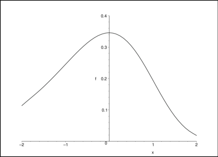
Figure 1: Precise solution for the size spectrum

This curve has a universal form which has been noticed in [1].

2 Iteration approximations

The iteration solution of eq. (1) was given in [3]. The recurrent procedure is defined as

$$g_{i+1}=c\int_{-\infty}^{z}(z-x)^{3}\exp(x-g_{i}(x))dx$$

with zero approximation $g_{0}=0$. The first iteration for $f(x)\sim\exp(x-g(x))$ has the following form

$$f_{1}\equiv\exp(x-pc\exp(x))$$

$$p=\int_{0}^{\infty}x^{3}\exp(-x)dx=6$$

$$pc=1.134$$

One can see that the first iteration is very close to the real precise solution which can be seen from Figure 2.

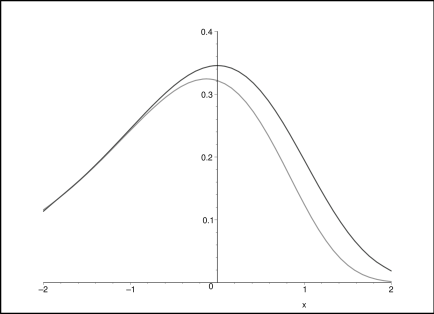
Figure 2: Precise solution and the first iteration for the size spectrum

The upper curve is the precise solution, the lower one is the first iteration.

One can see that the first iteration is already a good approximation. Now we shall formulate some new approximations with more simple physical sense.

3 Similarity of the embryos formation conditions

Under the conditions of the metastable phase decay one can see in [4] the similarity of conditions under which the embryos are appearing in the system. It was the consequence of the scale transformation of time. Here the situation seems to be another. The time explicitly stands in the term $\exp(x)$ for $f\sim\exp(x-g(x))$ which characterizes the action of external forces. Let us consider the subintegral expression in the integral calculated for the first iteration. The size $\rho_{dr}$ of the embryo can be expressed as

$$\rho_{dr}=\frac{\Phi^{2}_{*}}{\Gamma\tau d\Phi/dt}(z-x)$$

To observe the similarity we need to see the subintegral equation in the variable $\rho=z-x$. The subintegral function $g_{sub\ 1}$ in the expression for $g_{1}$ is the following

$$g_{sub\ 1}\sim\exp(z)\rho^{3}\exp(-\rho)$$

Factor $\exp(z)$ is not more than a scaling factor and we have the universal expression

$$g_{sub\ 1}\sim\rho^{3}\exp(-\rho)$$

for subintegral function in the first iteration. Because the first iteration resembles the precise solution we see that the last relation means that conditions for appearance of the droplets in different moments of time are similar, only the scaling factors change. Here it isn’t clear how to use this property, but in the direct investigation of stochastic effects this property will be very useful.

The universal form of $g_{sub\ 1}$ is drawn in Figure 3.

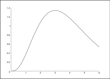
Figure 3: The universal form of subintegral expression for the first iteration for the size spectrum

We see that the maximum of subintegral expression is at $\rho=3$ and at $\rho=1.4\equiv\rho_{b}$ the half of the maximal height is attained. This value can be regarded as some characteristic boundary. The other boundary is $\rho=\rho_{c}=5.8$.

4 First iteration with shifted maximum

The value $c=0.189$ corresponding to the maximum at $x=0$ was established after explicit numerical solution of (1). One can pose a question what value of $c$ corresponds to the maximum of the first iteration at $x=0$. Certainly, this procedure will lead to $c=1/6$ and to a shifted first iteration

$$f_{1\ sh}\sim\exp(x-\exp(x))$$

This iteration coincides with precise solution even better than the previous first iteration. It can be seen from Figure 4.

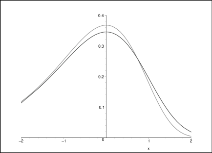
Figure 4: The form of precise solution and the shifted first iteration

There are two curves: the curve with sharp slope corresponds to the shifted first iteration and the curve with smooth slope corresponds to the precise solution.

5 Monodisperse approximation

Let us calculate expression for $g$ according to (1). We shall use a monodisperse approximation. We get

$$g=c\int_{-\infty}^{z}(z-x)^{3}\exp(x-g(x))\approx cNz_{max}^{3}$$

where $z_{max}$ is the coordinate of a monodisperse peak and $N$ is the number of droplets. For $N$ one can propose

$$N=\int_{-\infty}^{z}\exp(x-g)dx$$

For $z_{max}$ since the maximum occurs at $z=-3$ one can get

$$z_{max}=z+3$$

This forms the first variant of monodisperse approximation. It is not very precise because we have attributed the value $z+3$ to small droplets which are in a big quantity when we are near maximum of supersaturation. So, we have to correct our approximation.

The region of integration to calculate $N$ can be cut off at $\rho_{b}$. Then the renormalized number of droplets formed until maximum of supersaturation is

$$\hat{N}(z=0)=\int_{-\infty}^{-\rho_{b}}\exp(x-g)dx$$

For $\rho>\rho_{b}$ one can assume that $g$ is negligible. This leads to the possibility to use the ideal supersaturation instead of the real one. Then one can come to

$$N\approx\int_{\rho_{b}}^{\infty}\exp(-\rho)d\rho=\exp(-\rho_{b})=\exp(-1.4)$$

So, at every moment the number of droplets is $\exp(-1.4)\exp(z)$ and the coordinate of monodisperse spectrum is $x=3$. Then for $f\sim\exp(x-g)$ one can get

$$f\approx f_{mono\ 1}=\exp(x-3^{3}c\exp(-1.4)\exp(x))$$

Figure 5 illustrates this approximation, here the upper curve is the precise solution and the lower curve is the current approximation.

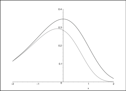
Figure 5: The form of monodisperse approximation $f_{mono\ 1}$.

The precision of approximation is satisfactory.

This was only one variant of monodisperse approximation. Now we shall present another variant. Note that at every moment one can say that the droplet corresponding to the maximum of subintegral equation (in the first iteration) has a size $\rho$ three units greater than a current size. This leads to

$$f\approx f_{mono\ 2}\equiv\exp(x-(x+3)^{3}\exp(-1.4)c)$$

The form of spectrum is drawn in Figure 6. The smooth hill corresponds to the approximation, the sharp hill corresponds to the precise numerical solution.

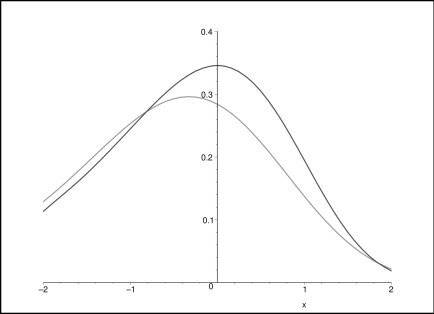
Figure 6: The form of monodisperse approximation $f_{mono\ 2}$

The precision of the last approximation is satisfactory.

6 Monodisperse approximation at the maximum of supersaturation

Earlier we constructed monodisperse approximations for every moment of time. Now we shall take into account that the main quantity of droplets will be formed near the maximum of supersaturation, i.e. near $z=0$. So, here we can put the position of monodisperse spectrum as $z=-3$. Then one can state that the maximum of the model spectrum

$$f\sim\exp(x-A(x+3)^{3})$$

with parameter $A$ has maximum at $z=0$. This gives $A=1/27$. Moreover one can move back from the shifted spectrum to the unshifted one by the substitution of $6c/27$ instead of $1/27$. Then one can come to

$$f\approx f_{mono\ 3}\equiv\exp(x-\frac{6c}{27}(x+3)^{3})$$

This spectrum together with the precise solution is drawn in Figure 7. Here the sharp curve corresponds to the precise solution and the smooth curve corresponds to the approximation. It is seen that they are practically similar.

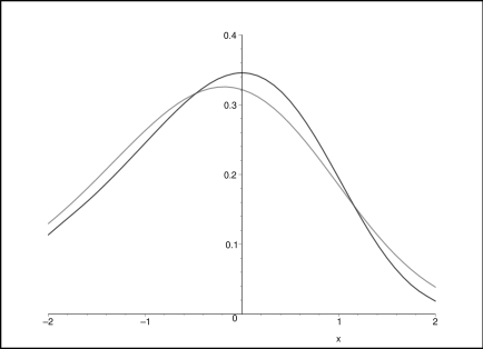
Figure 7: The form of monodisperse approximation $f_{mono\ 3}$

When $A=1/27$ one can come to

$$f\approx f_{mono\ 4}\exp(x-\frac{1}{27}(x+3)^{3})$$

This spectrum together with the precise solution is drawn in Figure 8. Here the lower curve corresponds to precise solution and the upper curve - to approximation. It is seen that they are also practically similar, especially their forms.

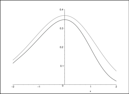
Figure 8: The form of monodisperse approximation $f_{mono\ 4}$

Instead of $N\sim\exp(-1.4)\exp(x)$ we put $N\sim 6c/27$ or $N\sim 1/27$ and conserve the fixed coordinate $x=3$.

The same can be done with approximations of the type $f_{mono\ 1}$ and $f_{mono\ 2}$ Then we come to

$$f_{mono\ 5}=\exp(x-\frac{6c}{27}\exp(x)3^{3})$$

and

$$f_{mono\ 6}=\exp(x-\frac{1}{27}\exp(x)3^{3})$$

We see that they coincide with $f_{mono\ 3}$ and $f_{mono\ 4}$. They are drawn in Figure 7 and Figure 8. So, we see that we can do the mentioned substitution at different steps of derivation.

7 Two stage scheme

The next approach to construct some approximations will be based on the property which results in applicability of the first iteration. What is the physical reason of applicability of the first iteration instead of the precise solution? The physical reason is the following: the embryos which are the main consumers of vapor were formed at initial moments of nucleation period when the supersaturation was near the ideal value. This allows us to extract the initial stage of nucleation period $z<-1$ and the second stage which is the whole nucleation period except the initial stage. The second stage is the stage when the main quantity of embryos was formed.

Really $g(-1)<c\exp(-1)$ is small in comparison with characteristic value of $g$ during the second stage $g\sim c$. So at $z<-1$ the supersaturation $\zeta$ is close to $\Phi$.

The influence of embryos appeared at initial stage on the evolution at the second stage is given through

$$a_{i}=\int_{-\infty}^{-1}x^{i}\exp(x-cg(x))dx\ \ i=0,1,2,3$$

Direct calculation on a base of the first iteration leads to

$$a_{0}=\exp(-1)$$

$$a_{1}=-2\exp(-1)$$

$$a_{2}=5\exp(-1)$$

$$a_{3}=-16\exp(-1)$$

Then

$$g\approx g_{in}\equiv c(x^{3}a_{0}-3x^{2}a_{1}+3xa_{2}-a_{3})$$

and the spectrum $f\sim\exp(x-g)=\exp(x-c(x^{3}a_{0}-3x^{2}a_{1}+3xa_{2}-a_{3}))$ is drawn in Figure 9 together with the precise solution which has more sharp form.

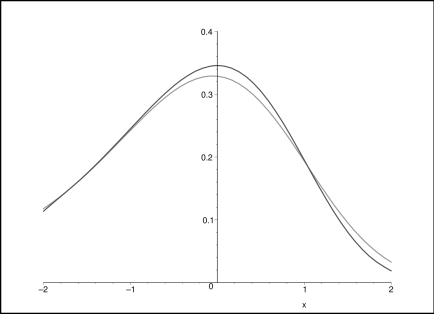
Figure 9: The form of approximation of two stages together with precise solution.

Here we forget that this expression takes place only for $z>-1$. We spread it for $z<-1$ because here the spectrum isn’t too high.

However, the asymptotic behaviour at $z\rightarrow-\infty$ will be qualitatively wrong. But as for the form of spectrum in a really significant region we see that the coincidence of two curves is practically ideal.

8 Balance property

The model forms of the size spectrum obtained above have to be self consistent. The self consistency can be treated at least in two senses. The first is the weak dependence of the total number of droplets on the number of droplets in the monodisperse peak. This question is separately analyzed directly in investigation of stochastic effects. Here we shall see the weak dependence of the total number of droplets on the position of the monodisperse peak or on the position of the boundary between two stages of the nucleation period.

We shall analyze two models - the model of the monodisperse peak and the model appeared in the two stage scheme. These models are the most precise ones.

We shall start with the model of the monodisperse peak. At first we shall generalize it. Let the monodisperse peak be formed at $z=-p$. Then instead of $A=1/27$ we have $A=1/(3p^{2})$. For the size spectrum we get

$$f\sim\exp(x-\frac{1}{3p^{2}}(x+p)^{3})$$

The total number of droplets we get the following expression

$$N_{tot}=N_{in}+\exp(-p)$$

where $N_{in}$ is the number of droplets appeared after $z=-p$. The last value can be calculated as

$$N_{in}=\int_{-p}^{\infty}\exp(x-\frac{1}{3p^{2}}(x+p)^{3})dx$$

In the renormalization adopted here the total number calculated on the base of precise solution is precisely equal to $1.00$. The numbers $N_{in}$ and $N_{tot}$ are drawn in Figure 10 as functions of $p$. It is clear that the dependence of $N_{tot}$ on $p$ is very weak one.

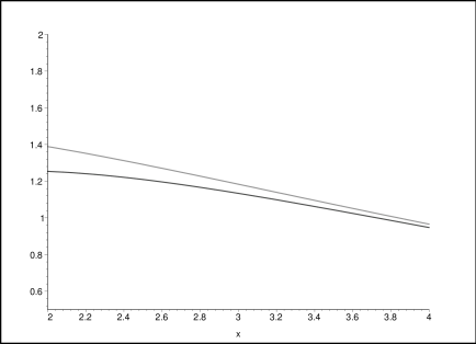
Figure 10: The values $N_{tot}$ and $N_{in}$ as functions of the position of monodisperse peak $p$.

The same we shall do for the model of the two stage approach. We shall state that before the boundary $z=-p$ the spectrum is the ideal one

$$f\sim\exp(x)$$

Fot $z$ greater than $-p$ the evolution is governed only by the substance accumulated in the droplets appeared before $z=-p$. This gives

$$f\sim\exp(x-c(x^{3}a_{0}-3x^{2}a_{1}+3xa_{2}-a_{3}))$$

where universal momentums are given by

$$a_{0}=\exp(-p)$$

$$a_{1}=-p\exp(-p)$$

$$a_{2}=p^{2}\exp(-p)+2p\exp(-p)+2\exp(-p)$$

$$a_{3}=-p^{3}\exp(-p)-3p^{2}\exp(-p)-6p\exp(-p)-6\exp(-p)$$

The total numbers of droplets $N_{tot}$ is equal to

$$N_{tot}=\exp(-p)+N_{in}$$

where $N_{in}$ is the number of droplets appeared after $z=-p$. The last value is given by

$$N_{in}=\int_{-p}^{\infty}\exp(x-c(x^{3}a_{0}-3x^{2}a_{1}+3xa_{2}-a_{3}))dx$$

The numbers $N_{in}$ and $N_{tot}$ are drawn in Figure 11 as functions of parameter $p$ of the boundary $z=-p$. One can see that the dependence of $N_{tot}$ on $p$ is very weak one. Moreover the number of droplets (which is always greater than the precise value $1.00$) has minimum at $p\sim 1$. Namely this value is the optimal one. We see that the value $p=0$ used in [5] is very far from the optimal one.

One can also note that this property of the weak dependence in deeply associated with constructions in the base of the modified gaussian method considered in [6].

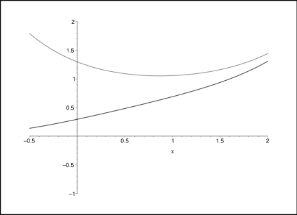
Figure 11: The values $N_{tot}$ and $N_{in}$ as functions of the position of the boundary $p$.

References

- [1] Kurasov V.B. Phys.Rev.E vol. 49, p. 3948 (1994)
- [2] Kuni F.M. The kinetics of the condensation under the dynamical conditions, Kiev, 1984, -65p. / Preprint Institute for Theoretical Physics Acad. of Sci. UkrSSR: ITP-84-178E
- [3] Kuni F.M., Grinin A.P. Kurasov V.B., Heterogeneous nucleation in the vapor flow, In: Mechanics of inhomogeneous liquids. Editor G.Gadiyak, Novosibirsk, 1986, p. 86
- [4] V. Kurasov Preprint cond-mat/0207024. Effects of stochastic nucleation in the first order phase transition
- [5] Grinin A.P., Kuni F.M., Sveshnikov A.M. Kolloidn. journ. v. 63, N 6, p. 747-754 (2001)
- [6] Kurasov V.B., VINITI 2592B95 from 19.09.95, 22p.