Present address: ] Department of Applied Physics, Yale University, New Haven, CT 06520

Photovoltaic and Rectification Currents in Quantum Dots

Abstract

We investigate theoretically and experimentally the statistical properties of dc current through an open quantum dot subject to ac excitation of a shape-defining gate. The symmetries of rectification current and photovoltaic current with respect to applied magnetic field are examined. Theory and experiment are found to be in good agreement throughout a broad range of frequency and ac power, ranging from adiabatic to nonadiabatic regimes.

Transport in mesoscopic systems subject to time-varying fields combines elements of non-equilibrium physics and quantum chaos. This combination extends the scope of mesoscopic physics and is likely to be important in quantum information processing, where fast gating and quantum coherence are both required. Of particular importance is the ability to control external fields applied to the mesoscopic system and to distinguish effects of these fields on quantum dynamics of the system. For example, two distinct contributions to direct current through an open quantum dot due to an oscillating perturbation have been identified Brouwer (1998, 2001) and observed experimentally in Ref. DiCarlo et al. (2003).

In this Letter, we investigate the statistical properties of dc currents resulting from an applied ac electric field over a wide range of excitation frequencies, paying particular attention to the presence or absence of symmetry with respect to magnetic field in various regimes. Theoretical analysis is based on recently developed time-dependent random matrix theory Vavilov and Aleiner (1999); Vavilov et al. (2001). Experiments use a gate-defined GaAs quantum dot subject to ac excitation of a gate at MHz to GHz frequencies. At low excitation frequencies $\omega\ll\tau_{\rm d}^{-1}$ ($\tau_{\rm d}$ is the electron dwell time in the dot) the present theoretical results are consistent with those obtained by adiabatic approximations Brouwer (1998); Shutenko et al. (2000). However, the analysis is applicable over a wider range of frequencies $\omega\lesssim E_{\rm T}$, where $E_{\rm T}=\hbar/\tau_{\rm cross}$ is the Thouless energy and $\tau_{\rm cross}$ is the electron crossing time of the dot. At higher frequencies $\omega\gtrsim E_{\rm T}$, the system may be studied by methods developed for bulk conductors Altshuler et al. (1982); Wang and Kravtsov (2001).

Three distinct contributions to dc current through the dot can be identified, resulting from: i) an applied dc bias; ii) an ac bias at the excitation frequency (i.e., rectification effects Brouwer (2001)); iii) photovoltaic effects Falko and Khmel’nitskii ; Vavilov et al. (2001). We restrict our attention to one-parameter excitation, noting that while in the adiabatic regime one- and two-parameter excitations affect the system differently, beyond the adiabatic regime, $\omega\gtrsim\tau_{\rm d}^{-1}$, the differences disappear Vavilov et al. (2001).

The Hamiltonian of electrons in the dot in the presence of a magnetic flux $\Phi$ is represented by a Hermitian $M\times M$ matrix $\hat{H}(t)=\hat{\cal H}_{\Phi}+\hat{\cal V}\cos\omega t$, with the time independent part $\hat{\cal H}_{\Phi}$ being a random realization of a matrix from a Gaussian unitary ensemble with the mean level spacing $\delta_{1}$, and $\hat{\cal V}$ being a matrix from a Gaussian orthogonal ensemble characterized by the strength $C_{0}=\pi{\rm Tr}\hat{\cal V}^{2}/M^{2}\delta_{1}$ and $M\delta_{1}\sim E_{\rm T}$ flo . The parameter $C_{0}$ determines the energy displacement of an electron state due to the applied perturbation $\hat{\cal V}$. The contact between the left (right) lead and the dot contains $N_{\rm l}$ ($N_{\rm r}$) open channels, we enumerate channels, $\alpha$, in the left ($\alpha=1\dots N_{\rm l}$) and the right ($\alpha=N_{\rm l}+1\dots N_{\rm ch}$) contacts, $N_{\rm ch}=N_{\rm l}+N_{\rm r}$. The corresponding experimental setup is shown in Fig. 1.

The dc current $\bar{I}^{\Phi}$ through the dot is determined by the scattering matrix $[{\cal S}_{\Phi}(t,t^{\prime})]_{\alpha\beta}$, see Ref. Vavilov et al. (2001):

$$\begin{split}\bar{I}^{\Phi}&=\frac{e\omega}{2\pi}\int\limits_{0}^{2\pi/\omega}dt\int\limits_{-\infty}^{+\infty}dt_{1}dt_{2}\\ &\times{\rm Tr}\left\{\hat{f}(t_{1},t_{2})\left[\hat{{\cal S}}^{\dagger}_{\Phi}(t_{2},t)\hat{\Lambda}\hat{{\cal S}}_{\Phi}(t,t_{1})-\hat{\Lambda}\delta_{t,t_{1}}\delta_{t,t_{2}}\right]\right\}.\end{split}$$ (1)

Here $\delta_{t,t^{\prime}}=\delta(t-t^{\prime})$ and

$$f_{\alpha\beta}(t,t^{\prime})=\frac{k_{\rm B}T}{\hbar}\frac{\delta_{\alpha\beta}\exp\left(i\frac{e}{\hbar}\int_{t^{\prime}}^{t}V_{\alpha}(\tau)d\tau\right)}{\sinh(\pi k_{\rm B}T(t-t^{\prime})/\hbar)}$$ (2)

is the distribution function of electrons in channel $\alpha$ at temperature $T$ and voltage $V_{\alpha}(t)$. At sufficiently low frequencies $\omega\ll E_{c}/\hbar$ ($E_{c}$ is the dot charging energy) $V_{\alpha}(t)$ is simply related to the bias $V(t)$ across the dot: $V_{\alpha}(t)=\Lambda_{\alpha\alpha}V(t)$. Elements of the diagonal matrix $\hat{\Lambda}$ are $\Lambda_{\alpha\alpha}=N_{\rm r}/N_{\rm ch}$ for $1\leq\alpha\leq N_{\rm l}$, and $\Lambda_{\alpha\alpha}=-N_{\rm l}/N_{\rm ch}$ for $N_{\rm l}<\alpha\leq N_{\rm ch}$.

We consider the bias $V(t)$ across the dot in the form $V(t)=V_{0}+V_{\omega}\cos(\omega t+\varphi_{1})$. The dc current through the dot to first order in dc bias $V_{0}$ and ac bias $V_{\omega}$ is non

$$\bar{I}^{\Phi}=\bar{I}^{\Phi}_{\rm ph}+\bar{I}_{1}^{\Phi}+\bar{g}^{\Phi}_{0}V_{0},\quad\bar{I}_{1}^{\Phi}=\bar{g}^{\Phi}_{1}V_{\omega},$$ (3)

where the first term represents the photovoltaic current $\bar{I}^{\Phi}_{\rm ph}=\bar{I}^{\Phi}(V_{\alpha}\equiv 0)$, see Eqs. (1) and (2). The second and third terms in Eq. (3) represent the contributions to the current due to dc bias $V_{0}$ and ac bias $V_{\omega}$, respectively:

$$\bar{g}_{0}^{\Phi}=\frac{e^{2}}{\pi\hbar}\left[G_{0}-\overline{\delta G_{0}^{\Phi}(t)}\right],\quad\bar{g}_{1}^{\Phi}=-\frac{e^{2}}{\pi\hbar}\overline{\delta G_{1}^{\Phi}(t)},$$ (4)

where $G_{0}=N_{\rm l}N_{\rm r}/N_{\rm ch}$ is the classical conductance and $\overline{\delta G_{k}(t)}=\int_{0}^{2\pi/\omega}\delta G_{k}(t)\omega dt/2\pi$ stands for time averaging of the “instantaneous conductance” ($k=0,1$)

$$\delta G_{k}^{\Phi}(t) = \int d\tau F_{k}(\tau)\int d\theta\cos(k(\omega\theta+\varphi_{k}))$$

$$\times \!{\rm Tr}\left\{\hat{\Lambda}\hat{{\cal S}}_{\Phi}^{\dagger}\left(\theta-\frac{\tau}{2},t\right)\hat{\Lambda}\hat{{\cal S}}_{\Phi}\left(t,\theta+\frac{\tau}{2}\right)\right\},$$

$$F_{0}(\tau) \!\!= \!\!\!\frac{\pi k_{\rm B}T\tau/\hbar}{\sinh(\pi k_{\rm B}T\tau/\hbar)},\ F_{1}(\tau)=\frac{2\pi k_{\rm B}T\sin(\omega\tau/2)}{\hbar\omega\sinh(\pi k_{\rm B}T\tau/\hbar)}.$$

We observe that $\overline{\delta G_{1}(t)}=\overline{\delta G_{0}(t)\cos(\omega t+\varphi_{1})}$ in the adiabatic limit $\hbar\omega\ll{\rm max}\{N_{\rm ch}\delta_{1},k_{\rm B}T\}$ considered in Refs. Brouwer (2001); Moskalets and Buttiker (2003).

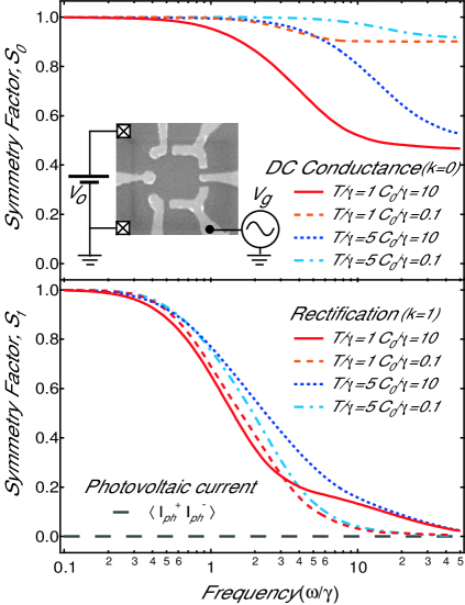
Figure 1: Symmetry factor $S_{k}=\langle\overline{\delta G_{k}^{+\Phi}}\ \overline{\delta G_{k}^{-\Phi}}\rangle/\langle(\overline{\delta G_{k}^{\Phi}})^{2}\rangle$ as a function of frequency $\omega$ for $k=0$ (upper panel) and $k=1$ (lower panel) at two values of temperature $T$ and power $C_{0}$ of the ac excitation. Inset: Micrograph of device and schematic picture of applied voltages.

Below we study the variance of the photovoltaic current $\bar{I}_{\rm ph}^{\Phi}$ and the conductances $\bar{g}_{0}^{\Phi}$ and $\bar{g}_{1}^{\Phi}$ with respect to random realizations of the Hamiltonian $\hat{\cal H}_{\Phi}$. Following Refs. Vavilov et al. (2001); Vavilov and Aleiner (2001), we find in the limit $N_{\rm ch}\gg 1$ and at magnetic fields $\Phi\gg\Phi_{0}\sqrt{N_{\rm ch}/M}$ destroying the weak localization ($\Phi_{0}=hc/e$)

$$\big{\langle}\!\!\left(\bar{I}_{\rm ph}^{\Phi}\right)^{\!2}\!\big{\rangle}=\frac{G_{0}e^{2}\omega^{4}C_{0}\delta_{1}}{2\pi^{3}\hbar^{2}}\!\!\!\!\!\int\limits_{0}^{2\pi/\omega}\!\!\!\frac{dtdt^{\prime}}{4\pi^{2}}\!\!\int\limits_{0}^{\infty}\!\!d\tau\!\!\!\int\limits_{\tau/2}^{\infty}\!\!\!d\theta\!K^{+}B^{\rm ph}_{t-\theta,t^{\prime}-\theta;\tau},$$ (6)

$$\big{\langle}\!\overline{\delta G_{k}^{+\Phi}}\ \overline{\delta G_{k}^{\pm\Phi}}\!\big{\rangle}=\frac{G_{0}^{2}\omega^{2}\delta_{1}^{2}}{2\pi^{2}\hbar^{2}}\!\!\!\!\int\limits_{0}^{2\pi/\omega}\!\!\frac{dtdt^{\prime}}{4\pi^{2}}\!\!\!\int\limits_{0}^{\infty}\!\!d\tau\!\!\int\limits_{\tau/2}^{\infty}\!\!d\theta\,K^{\pm}B^{(k)}_{t-\theta,t^{\prime}-\theta;\tau}$$ (7)

and $\langle\bar{I}^{+\Phi}_{\rm ph}\bar{I}^{-\Phi}_{\rm ph}\rangle=0$, see Ref. Shutenko et al. (2000). In Eqs. (6) and (7) the angle brackets $\langle\dots\rangle$ stand for the averaging with respect to realizations of $\hat{\cal H}_{\Phi}$. Functions $B^{(k)}_{t,t^{\prime};\tau}$ and $B^{\rm ph}_{t,t^{\prime};\tau}$ describe the distribution function foo (a) of electrons in the dot in the presence of time-dependent electric fields and kernels $K^{\pm}\equiv K^{\pm}_{t,t^{\prime};\theta,\tau}$ describe the evolution of electron states foo (b) in these fields. Both functions $B^{(k)}_{t,t^{\prime};\tau}$ and $B^{\rm ph}_{t,t^{\prime};\tau}$ and the kernels $K^{\pm}_{t,t^{\prime};\theta,\tau}$ contain the diffuson ${\cal D}(t_{1},t_{2},\tau)=\exp\left(-\int_{t_{2}}^{t_{1}}\Gamma(\tau,t)dt\right)$ or the Cooperon ${\cal C}(\tau_{1},\tau_{2},t)=\exp\left(-\frac{1}{2}\int_{\tau_{2}}^{\tau_{1}}\Gamma(\tau,t)d\tau\right)$. Here, $\Gamma(\tau,t)=\gamma_{\rm e}+\gamma_{\varphi}+4C_{0}\sin^{2}\omega t\sin^{2}(\omega\tau/2)$, where $\gamma_{\rm e}=\delta_{1}N_{\rm ch}/2\pi$ is the electron escape rate and $\gamma_{\varphi}$ is the electron phase relaxation rate due to inelastic processes.

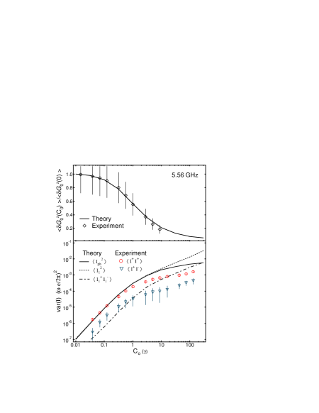
Figure 2: Upper panel: Variance of the conductance as a function of the ac excitation power $P=P_{0}C_{0}/\gamma_{\rm e}$ at $\omega/2\pi=5.56\$GHz ($\hbar\omega=7.2\gamma_{\rm e}$) and the theoretical result of Eq. (7) with $k=0$. We use $P_{0}=9\times 10^{-8}\$W and $k_{\rm B}T=5.4\gamma_{\rm e}$. Lower panel: Symmetric ($\bigcirc$) and antisymmetric ($\bigtriangledown$) current correlators as a function of ac excitation strength $C_{0}$. Solid line shows variance of the photovoltaic current Eq. (6) with parameters fixed by the fit in the upper panel. The dashed and dotted lines show the symmetric and antisymmetric correlators of the rectification current Eq. (8) with $\alpha_{\omega}=0.45\hbar\omega/e$ and $\varphi_{1}=0$.

In the experiment, the ac bias $V_{\omega}$ results from capacitive coupling between the leads and the gate on which the ac voltage is applied (see the inset in Fig. 1). Therefore $V_{\omega}$ is proportional to the amplitude of the ac voltage at the gate. Assuming that $C_{0}$ is linear in the applied power to the gates, we write $V_{\omega}=\alpha_{\omega}\sqrt{C_{0}/\gamma_{\rm e}}$. The coefficient $\alpha_{\omega}$ has units of voltage and is independent of realizations of the quantum dot (we disregard fluctuations of $\hat{\cal V}$ over different realizations of $\hat{\cal H}_{\Phi}$). Therefore, the correlation functions of the rectification current $\bar{I}^{\Phi}_{1}=\bar{g}_{1}^{\Phi}V_{\omega}$ are determined by the correlators of $\overline{\delta G_{1}^{\Phi}}$:

$$\Big{\langle}\bar{I}^{+\Phi}_{1}\bar{I}^{\pm\Phi}_{1}\Big{\rangle}=\frac{e^{4}}{\pi^{2}\hbar^{2}}\alpha_{\omega}^{2}\ \frac{C_{0}}{\gamma_{\rm e}}\ \Big{\langle}\overline{\delta G^{+\Phi}_{1}}\ \overline{\delta G^{\pm\Phi}_{1}}\Big{\rangle}.$$ (8)

We also notice that in the limit $N_{\rm ch}\gg 1$ the correlation function of the photovoltaic current $\bar{I}_{\rm ph}^{\Phi}$ and the rectification current $\bar{I}_{1}^{\Phi}$ vanishes Shutenko et al. (2000).

First we use Eqs. (7) and (8) to analyze the magnetic field symmetry of the rectification current $\bar{I}_{1}^{\Phi}$. Although in the adiabatic limit $\omega\ll\gamma_{\rm e}/\hbar$ the rectification current $\bar{I}_{1}^{\Phi}$ is symmetric with respect to magnetic field inversion ($\Phi\to-\Phi$), at higher frequencies $\omega\gtrsim\gamma_{\rm e}/\hbar$ the symmetry of $\bar{I}_{1}^{\Phi}$ is suppressed. Indeed, the magnetic field symmetry is related to the time inversion symmetry. For a harmonic field at frequency $\omega$, the time-inversion symmetry holds only on time scales much smaller than $1/\omega$. Transport through the system is determined by times of the order of $\hbar/\gamma_{\rm e}$ and consequently the magnetic field symmetry of the rectification current breaks if $\hbar\omega\gtrsim\gamma_{\rm e}$. We plot the ratio $S_{1}=\langle\overline{\delta G_{1}^{+\Phi}}\ \overline{\delta G_{1}^{-\Phi}}\rangle/\langle(\overline{\delta G_{1}^{\Phi}})^{2}\rangle$ as a function of $\hbar\omega/\gamma_{\rm e}$ in Fig. 1. $S_{1}=1$ represents the symmetric current $\bar{I}_{1}^{\Phi}\propto\overline{\delta G_{1}^{\Phi}}$ with respect to magnetic field inversion. In the adiabatic regime this symmetry originates from the Onsager symmetry Onsager of the dc conductivity, see Eq. (Photovoltaic and Rectification Currents in Quantum Dots) and Refs. Brouwer (2001); DiCarlo et al. (2003). As the frequency increases, $S_{1}$ vanishes, signalling the suppression of the magnetic field symmetry. Therefore, the absence of magnetic field symmetry no longer serves as a distinct feature of the photovoltaic current $\bar{I}_{\rm ph}^{\Phi}$, which allows one to distinguish $\bar{I}_{\rm ph}^{\Phi}$ and the rectification current $\bar{I}_{1}^{\Phi}$.

We notice that the magnetic field symmetry of the dc conductance $\overline{\delta G_{0}^{\Phi}}$ is more sturdy than the symmetry of the rectification current, see Fig. 1. Particularly, at temperatures $k_{\rm B}T\gtrsim\gamma_{\rm e}$, dc conductance $\overline{\delta G_{0}^{\Phi}}$ is nearly symmetric at frequencies $\hbar\omega\lesssim k_{\rm B}T$, since the dc correlation function is determined by processes on a time scale $\hbar/k_{\rm B}T$. The symmetry is not fully suppressed even at $\omega\gg k_{\rm B}T/\hbar$; the suppression depends on $C_{0}/\gamma_{\rm e}$.

We apply Eqs. (6) - (8) to the analysis of the experiment DiCarlo et al. (2003). The quantum dot used in the experiment has an area $A\approx 0.7$ $\mu$m². Relevant energy scales are the Thouless energy $E_{\rm T}\approx 160$ $\mu$eV and the mean level spacing $\delta_{1}=\pi\gamma_{\rm e}\approx 10$ $\mu$eV. The measurements were performed at the base electron temperature $T\approx 200$ mK ($k_{\rm B}T=5.4\gamma_{\rm e}$). From the size of conductance fluctuations without ac fluctuation on the gate, we estimate the dephasing rate $\gamma_{\varphi}\approx 0.2\gamma_{\rm e}$ (see Huibers (1999) for details) and thus disregard it in our quantitative analysis.

In the upper panel of Fig. 2 we show the variance of the conductance as a function of the incident power $P$ at $\omega/2\pi=5.56$ GHz ($\hbar\omega/\gamma_{\rm e}\approx 7.2$). We also plot the variance of the conductance calculated from Eq. (7) ($k=0$) at temperature $T=5.4\gamma_{\rm e}/k_{\rm B}$. Assuming that the ratio $C_{0}/\gamma_{\rm e}$ is proportional to the power $P$ of the ac excitation applied to the gate, i.e. $C_{0}/\gamma_{\rm e}=P/P_{0}$, we rescale $P$ to obtain the best fit of the experimental points by the curve of Eq. (7). We find $P_{0}=9\times 10^{-8}$ W.

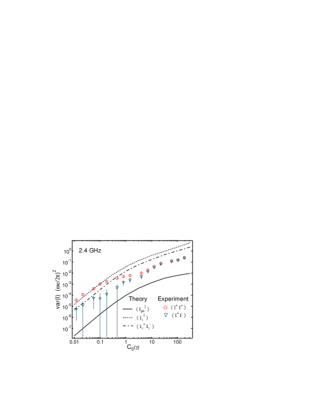
Figure 3: Symmetric ($\bigcirc$) and antisymmetric ($\bigtriangledown$) current correlators at $\omega/2\pi=2.4\$GHz as a function of power $P=P_{0}C_{0}/\gamma_{\rm e}$ with $P_{0}=2.5\times 10^{-7}\$W. Solid line shows variance of the photovoltaic current Eq. (6) at temperature $T=5.4\gamma_{\rm e}/k_{\rm B}$ and frequency $\omega=3.1\gamma_{\rm e}/\hbar$. The dashed and dotted lines show the symmetric and antisymmetric correlators of the rectification current Eq. (8) with $\alpha_{\omega}=4.7\hbar\omega/e$ and $\varphi_{1}=0$.

In the lower panel of Fig. 2 we show the correlators $\langle\bar{I}^{+\Phi}\bar{I}^{\pm\Phi}\rangle$ of the measured current. Although the traces of the magnetic field sweeps look quite asymmetric for the measured current, the antisymmetric correlator $\langle\bar{I}^{+\Phi}\bar{I}^{-\Phi}\rangle$ is not significantly smaller than its symmetric counterpart. We notice however, that if the averaging is performed over $n$ realizations, the measured correlator $\langle\bar{I}^{+\Phi}\bar{I}^{-\Phi}\rangle$ can be estimated as $\langle\bar{I}^{+\Phi}\bar{I}^{+\Phi}\rangle/\sqrt{n}$ ($n\sim 50$ in the experiment).

We plot the variance of the photovoltaic current, Eq. (6), as a function of $C_{0}/\gamma_{\rm e}$ for $k_{\rm B}T=5.4\gamma_{\rm e}$ and $\hbar\omega=7.2\gamma_{\rm e}$ (to facilitate numerics, we used the approximation $\hbar\omega\gg\gamma_{\rm e}$). We emphasize that the horizontal shift between the data points and curve is fixed by the fit in the upper panel for the dc conductance and there is no fitting parameters for the variance of the current (along vertical axis). At $C_{0}\lesssim\gamma_{\rm e}$, the variance of the measured current changes quadratically in $C_{0}/\gamma_{\rm e}$, consistent with quadratic dependence on $C_{0}$ of the theoretical curves for $\langle\bar{I}_{\rm ph}^{2}\rangle$ and therefore our assumption that $C_{0}$ is proportional to the power of the ac excitation is justified. At $C_{0}\gtrsim\gamma_{\rm e}$ the variance of the measured current starts saturating. This saturation is expected for large power asymptote of the photovoltaic current due to spreading of the distribution function of electrons in the dot Vavilov et al. (2001). Some deviation between the experimental points and the theoretical curve is expected due to the approximation $N_{\rm ch}\gg 1$ used for derivation of Eq. (6) ($N_{\rm ch}=2$ in the experiment).

For illustration, we also plot the correlation functions of the rectification current, using Eq. (8) for $\varphi_{1}=0$ and $\alpha_{\omega}=0.45\hbar\omega/e$. For the rectification current, the saturation at large power is not expected: according to Fig. 2, $\langle\bar{I}_{1}^{+\Phi}\bar{I}_{1}^{\pm\Phi}\rangle\propto(C_{0}/\gamma_{\rm e})^{a}$ with $a\approx 0.6$.

We similarly discuss the data for $\omega/2\pi=2.4$ GHz. Performing the fit of the experimental values of the conductance fluctuations and the result of Eq. (7) with $k=0$ and temperature $T=5.4\gamma_{\rm e}/k_{\rm B}$, we find the relation between the strength of the perturbation $C_{0}$ and the power $P=P_{0}C_{0}/\gamma_{\rm e}$ with $P_{0}=2.5\times 10^{-7}$ W.

In Fig. 3 we show the symmetric and antisymmetric current correlators for $2.4$ GHz. For comparison we plot by a solid line the variance of the photovoltaic current $\bar{I}_{\rm ph}^{\Phi}$, calculated from Eq. (6) at $\omega=3.1\gamma_{\rm e}$. We observe that the fluctuations of the measured current significantly exceed (by a factor $\sim 100$) the expected magnitude for the photovoltaic current, and therefore are likely due to the rectification of the bias across the dot. The low power data can be fitted by Eq. (8) with $\alpha_{\omega}=4.7\hbar\omega/e$.

The above choice for $\alpha_{\omega}\gtrsim\{\hbar\omega,k_{\rm B}T\}/e$ limits the applicability of the linear expansion Eq. (3) to small powers of the ac excitation $C_{0}$, such that $C_{0}/\gamma_{\rm e}\lesssim(\hbar\omega/e\alpha_{\omega})^{2}$. The higher order corrections in the bias $V_{\omega}$ do not restore magnetic field symmetry, which is in apparent contradiction to the observed symmetry of the measured current at larger powers (at $C_{0}/\gamma_{\rm e}\gtrsim 1$ in Fig. 3). We attribute the restoration of magnetic field symmetry to dephasing due to dot heating by the dissipative current. Increasing the power $P$ at fixed $\omega$ drives the system into the adiabatic regime since the heating makes the ratio $\hbar\omega/(\gamma_{\rm e}+\gamma_{\varphi})$ decrease. As shown already in Fig. 1, the rectification current is symmetric in the adiabatic regime. The assumption that $\gamma_{\varphi}$ increases as power $P$ increases is consistent with the observed change of the correlation field for the current fluctuations, see Fig. 4 in Ref. DiCarlo et al. (2003).

In summary, we studied ensemble fluctuations of dc current through an open quantum dot subject to oscillating perturbation. We showed that as frequency of the perturbation increases, magnetic field symmetry of the current disappears, regardless of the mechanism of the current generation. We demonstrated that the power behavior of the current fluctuations is an important tool to distinguish effects of an ac excitation on dc current.

We thank I. Aleiner, P. Brouwer, and V. Falko for useful discussions, and M. Hanson and A. C. Gossard at UC Santa Barbara for high-quality heterostructure materials used in the experiments. The work was supported by NSF grants DMR 02-13282 and DMR 0072777, and by AFOSR grant F49620-01-1-0475.

References

Brouwer (1998)
P. W. Brouwer,
Phys. Rev. B 58,
R10135 (1998).
Brouwer (2001)
P. W. Brouwer,
Phys. Rev. B 63,
121303 (2001).
DiCarlo et al. (2003)
L. DiCarlo,
C. M. Marcus,
and J. S.
Harris, Phys. Rev. Lett.
91, 246804
(2003).
Vavilov and Aleiner (1999)
M. G. Vavilov and
I. L. Aleiner,
Phys. Rev. B 60,
R16311 (1999).
Vavilov et al. (2001)
M. G. Vavilov,
V. Ambegaokar,
and I. L.
Aleiner, Phys. Rev. B
63, 195313
(2001).
Shutenko et al. (2000)
T. A. Shutenko,
I. L. Aleiner,
and B. L.
Altshuler, Phys. Rev. B
61, 10366 (2000).
Altshuler et al. (1982)
B. L. Altshuler,
A. G. Aronov,
D. E. Khmelnitskii,
and A. I.
Larkin, Quantum Theory of Solids
(Mir publisher, Moscow,
1982).
Wang and Kravtsov (2001)
X.-B. Wang and
V. E. Kravtsov,
Phys. Rev. B 64,
033313 (2001).
(9)
V. I. Falko and
D. E. Khmel’nitskii,
Zh. Eksp. Teor. Fiz. 95, 328, (1989), [Sov.
Phys. JETP 68, 186 (1989)].
(10)
Alternative methods to the time-dependent random
matrix theory here are based on Floquet approach, see M. Moskalets and
M. Büttiker, Phys. Rev. B 66, 205320 (2002), or time-dependent
scattering matrix approach, see M.L. Polianski and P.W. Brouwer,
J. Phys. A: Math. Gen. 36, 3215 (2003).
(11)
The biased current produces heating, and the analysis
beyond the linear response in the bias voltage requires consideration of heat
relaxation in the system.
Moskalets and Buttiker (2003)
M. Moskalets and
M. Büttiker,
Phys. Rev. B 69,
205316 (2004).
Vavilov and Aleiner (2001)
M. G. Vavilov and
I. L. Aleiner,
Phys. Rev. B 64,
085115 (2001).
foo (a)
and
.
foo (b)
and .
(16)
L. Onsager,
Phys. Rev. 38, 2265 (1931); M. Büttiker,
Phys. Rev. Lett. 57, 1761 (1986).
Huibers (1999)
A. G. Huibers, J.A. Folk, S.R. Patel,
C.M. Marcus, C.I. Duruöz, and J.S. Harris, Phys. Rev.
Lett. 83, 5090
(1999).