Glassy behaviour in an exactly solved spin system with a ferromagnetic transition

Abstract

We show that applying simple dynamical rules to Baxter’s eight-vertex model leads to a system which resembles a glass-forming liquid. There are analogies with liquid, supercooled liquid, glassy and crystalline states. The disordered phases exhibit strong dynamical heterogeneity at low temperatures, which may be described in terms of an emergent mobility field. Their dynamics are well-described by a simple model with trivial thermodynamics, but an emergent kinetic constraint. We show that the (second order) thermodynamic transition to the ordered phase may be interpreted in terms of confinement of the excitations in the mobility field. We also describe the aging of disordered states towards the ordered phase, in terms of simple rate equations.

Despite many years of study of glass-forming liquids, the most suitable paradigm in which to discuss the ‘glass transition’ and its associated dynamical phenomena remains controversial. In recent years, there has been progress GCTheory ; Berthier2003 ; Whitelam2004 , driven by the idea that the dynamical properties of glass-formers may be characterised by a zero temperature dynamical fixed pointWhitelam2004 . This is in contrast to the predictions of other theories which involve a finite temperature singularity in the dynamics MCT ; Biroli-Bouchaud or the thermodynamics of the relevant systemTarjus-Kivelson ; Xia-Wolynes ; Mezard-Parisi .

However, there remains an important qualitative difference between physical glass-formers and the models, such as the Fredrickson-Andersen (FA)FAModel or EastEastModel models (see Ritort-Sollich for a review) studied in GCTheory ; Berthier2003 ; Whitelam2004 : the crystal phase is completely absent from these models. As a result, they are relevant if the glass-forming liquid is in a long-lived (but metastable) supercooled phase. Further, interplay between the thermodynamic singularity associated with the transition to the crystal and the dynamical fixed point associated with the glass is certainly possible, but the FA and East models cannot capture these phenomena since their thermodynamics are trivial. There has been recent workCavagna2003 ; Franz2001 (see also Swift2000 ) investigating these issues with regard to glassy systems, although without reference to a glassy fixed point at zero temperature.

The extent to which the FA and East models can be viewed as pictures of real glasses is therefore contingent on two main assumptions. Firstly, the behaviour of the supercooled state should not be affected by the proximity of the freezing transition, since the FA and East models regard glassy slowing down as a purely dynamical effect, not requiring a thermodynamic transition. Secondly, the ‘mobility field’ represented by the spins in these models should emerge naturally from atomistic degrees of freedom of the glass-former.

One class of models in which this latter effect is demonstrated are the two-dimensional plaquette models Lipowski ; Garrahan-Newman ; barca , in which an effective dynamical constraint emerges naturally from a simple spin model. There are free excitations in the spin field which are naturally interpreted as a mobility field. At temperatures lower than the glassy onset temperature, $T_{o}$ Brumer ; Berthier2003 , the dynamics are strongly heterogeneous, and slow down rapidly with decreasing temperature.

In this paper, we address the other issue mentioned above: how are dynamics of metastable supercooled states affected by the presence of the freezing transition? We study dynamics in the eight-vertex model, whose thermodynamics were solved by BaxterBaxterBook . The model may be treated as a generalisation of the square plaquette model Lipowski ; barca ; the effect of this generalisation is to to introduce a (second order) phase transition to an ordered state at a finite temperature $T_{c}$. We identify this with a freezing transition, and investigate the dynamics around this transition. The transition temperature $T_{c}$ may be varied with respect to the glassy onset temperature $T_{o}$. This fact, together with the exactly solved thermodynamics, gives an extra degree of control to our simulations.

We will show that we may prepare long-lived ‘supercooled’ states below $T_{c}$, whose dynamics are controlled by the effective dynamical constraint of the plaquette model, and are not affected by the freezing transition for times shorter than the lifetime of the supercooled state.

To be more precise, the dynamics of the system within the supercooled state resemble those of strong glasses, and arise from diffusing point-like excitations in a mobility field GCTheory ; Whitelam2004 ; Berthier2003 . Considering supercooled states at different temperatures, we find that they obey dynamical scaling consistent with a zero temperature fixed point. The presence of the ferromagnetic transition means that these states have a finite lifetime, but it does not affect the dynamics on timescales shorter than this lifetime. This is consistent with the assumptions made when modelling glass-formers using models without an ordering transition GCTheory ; Whitelam2004 ; Berthier2003 .

The form of the paper is as follows: in section I, we describe the model, identify relevant energy scales and their hierarchy, and discuss the relation between the spins of our model and the atomistic degrees of freedom of a physical glass former. We discuss the nature of the ordered and disordered phases of the model system in section II: we then use this information to interpret simulations of the dynamics of the model in section III. Finally, we summarise our results in section IV, and discuss their significance for models of the glass transition.

I The model

The zero-field eight vertex model, solved by BaxterBaxterBook may be expressed either in terms of its original vertices, or as an Ising model with Hamiltonian:

$$H =\sum_{ij} \left[-D\sigma_{ij}\sigma_{i+1,j}\sigma_{i,j+1}\sigma_{i+1,j+1}\right.$$ (1)

$$\left.-J\left(\sigma_{ij}\sigma_{i+1,j+1}+\sigma_{i+1,j}\sigma_{i,j+1}\right)\right]$$

where the $\{\sigma_{ij}\}$ are Ising spins on a square lattice. We note that the Ising coupling is between next nearest neighbours on the square lattice: at $D=0$ there are two independent sublattices, with Ising coupling, $J$ within each sublattice. There is a transition at $J=(T/2)\sinh^{-1}(1)$ to a fourfold degenerate ordered state (there are two ferromagnetic and two antiferromagnetic ground states, related by flipping all the spins on either sublattice). As $D$ is increased from zero, the lattices become coupled, and the transition moves to a higher temperature: the critical temperature $T_{c}$ satisfies:

$$\sinh(2J/T_{c})=\exp(-2D/T_{c})$$ (2)

The transition to an ordered state occurs for all finite $J$: we also note that if $D>J$ then the transition temperature will be much larger than $J$.

Thus far we have considered only static (thermodynamic) properties of the eight-vertex model. In order to study the time evolution of the this model, we must specify dynamical rules. We use simple spin flips with rates given by Glauber dynamics. We refer to the combination of the Hamiltonian and the dynamical rules as the spin-flip eight vertex (SEV) model.

If we set $J=0$ in the SEV model, we arrive at the (two dimensional) plaquette modelLipowski ; Buhot2002 ; Espriu2003cm . In this limit there is no ordering at any finite temperature: all two point static correlations vanish. This may be most easily demonstrated by noting that if $J=0$ then the Hamiltonian is invariant under flipping all of the spins in any row or column of the square lattice. The dynamics of this model are dominated by a zero temperature dynamical fixed point for temperatures $T$ that are small compared to $D$. Since we are studying slow dynamics we work throughout at $T<D$.

We have now identified two temperature scales in the problem: the onset of glassy dynamics occurs at $T=T_{o}\sim D$ and the critical point in the system is at $T=T_{c}$. If $T_{c}>T_{o}$ then we expect the slow dynamics to be observable only in the ordered phase: the more interesting case is $T_{o}>T_{c}$, in which case the dynamics are slow near the transition, and we may investigate the effect of the effective kinetic constraint as we cool the system through $T_{c}$. We therefore work at $T_{c}<D$: from (2), this means that $J<T_{c}$. As a result we have the hierarchy $J<(T,T_{c})<D$ which is obeyed throughout this paper.

I.1 Relation of this work to physical glass formers

Before investigating the SEV model more closely, we establish the relationship between this model and physical glass-formers: it is not obvious at first sight precisely how a model of Ising spins should be related to a atomistic system. The spin variables represent the microscopic degrees of freedom of the glass-former. This is distinct from the more heuristic approach taken in the FA and East models in which the spins represent a coarse-grained ‘mobility field’. The SEV model is more similar to the plaquette modelbarca in that the effective kinetic constraint responsible for the critical slowing down at zero temperature is not inserted explicitly, but arises from the combination of the Hamiltonian and simple spin-flip dynamics. In section III we will comment briefly on how the dynamics may be interpreted within a ‘mobility field’ picture like that of the FA model.

In the previous section we identified the two temperature scales in the model as the glassy onset temperature $T_{o}\sim D$ and the transition temperature $T_{c}<T_{o}$. These separate the behaviour of the system into three regimes. We argue that the high temperature phase of the SEV model with $T>(T_{o},T_{c})$ resembles a liquid-like state of the atomistic system, since it lacks any two point correlations between the spins.

The second regime is $T_{c}<T<T_{o}$: there are still no static correlations between the spins but there are strong dynamical correlations. This state resembles a viscous liquid whose relaxation time is large compared to microscopic timescales. We emphasise that the crossover between this regime and the high temperature behaviour is smooth: there is no sharp transition at $T_{o}$. In the viscous liquid, the atomistic degrees of freedom are ‘jammed’ over large regions of the system: relaxation in these regions is frustrated by large energy barriers. Dynamical heterogeneity then arises naturally, due to the presence of mobile regions where the energy barriers are smaller than average. There are very many paramagnetic states in the spin system, even at low temperatures (compared to $D$): these resemble the many possible jammed states of the glass former.

Having argued that the paramagnetic phase of our model is liquid-like, and shows glassy behaviour at low temperatures, it is natural to interpret the transition in the model as a a freezing transition. We identify the ferromagnetic phase with the crystalline states of the glass-former. As the temperature is lowered through $T_{c}$ the entropy falls rapidly as the very many paramagnetic (jammed) states are now thermodynamically unstable with respect to the ferromagnet. The effect of the dynamical fixed point on the transition between paramagnet and ferromagnet is the main subject of the following sections. In particular we show that ‘supercooling’ of the paramagnetic state is possible as long as $T_{c}\ll D$.

II Static properties of the SEV model

Figure 1: Sketch showing the relation between spin states, excited plaquettes and domain walls. Up (down) spins are represented by filled (empty) circles. Domain walls form closed loops with excited plaquettes (energy cost $2D$) at each isolated corner (there is no energy cost associated with wall crossings). A domain wall costs energy $2J$ per unit length when running though a ferromagnetically ordered region. Interactions between domain walls reduce this tension in disordered states.

We now discuss the microscopic structure of the ferromagnetic and paramagnetic states in the model of equation (1). This will allow us to identify the relevant correlation functions for our study of the dynamics of the system. We describe the paramagnetic state in terms of small deviations from the behaviour of the model with $J=0$, and the ferromagnetic state in terms of excitations in an ordered background. This will lead us to interpret the transition in terms of free defects above $T_{c}$ that become confined at the transition, forming composite excitations. We will also show that these descriptions are valid even rather close to the transition, despite being based on expansions around the fully ordered or fully disordered states. In other words, the critical region is very narrow.

We begin by recalling some results for the $J=0$ limit of the modelBuhot2002 ; Espriu2003cm . At $J=0$, we write $p_{i}=\sigma_{ij}\sigma_{i,j+1}\sigma_{i+1,j}\sigma_{i+1,j+1}$, and the Hamiltonian reduces to

$$H_{J=0}=-D\sum_{i}p_{i}$$ (3)

where the $p_{i}$ are Ising-like degrees of freedom, defined on the plaquettes of the square lattice. In the thermodynamic limit, these plaquettes are independent degrees of freedom, that define the state of the spin system, up to transformations that flip all the spins in any row or column (leaving $H_{J=0}$ invariant). We observe that this results in a ground state entropy proportional to the linear size of the system, $L$ (there are $N=L^{2}$ spins in the system).

In finite systems, the presence of boundary conditions may impose constraints on the plaquettes. For example, imposing periodic boundaries on the spins means that the number of excited plaquettes in all rows and columns must be even (we believe that this fact led to the strong finite size effects seen in Espriu2003cm ).

As discussed in Espriu2003cm , the low temperature states of the model with $J=0$ are best interpreted in terms of closed loops with excited plaquettes at each vertex (see figure 1). If we move across the lattice, any spin flip is accompanied by our crossing the perimeter of a loop. If $J=0$ then each plaquette is independent: the vertices of the loops are a free lattice gas with density $(1+e^{2D/T})^{-1}$. The free energy per site is simply

$$f_{J=0}=-T\log[2\cosh(D/T)]$$ (4)

At finite $J$, we make use of Baxter’s solution of the eight vertex modelBaxterBook . In appendix A, we show that the free energy per site for $T\gg T_{c}$ is given approximately by

$$f_{\mathrm{pm}}^{(0)}=-T\log\left[e^{D/T}\cosh(2J/T)+e^{-D/T}\right]$$ (5)

Since we work exclusively at $J<T$, equation (5) is rather close to the $J=0$ expression (4).

We focus on two correlation functions, the density of excited plaquettes $n_{p}$, and the density of broken Ising bonds, $n_{b}$. Their definitions are:

$$n_{p} = \frac{1}{2}(1-\langle\sigma_{ij}\sigma_{i,j+1}\sigma_{i+1,j}\sigma_{i+1,j+1}\rangle)$$ (6)

$$n_{b} = \frac{1}{4}(2-\langle\sigma_{ij}\sigma_{i+1,j+1}+\sigma_{i+1,j}\sigma_{i,j+1}\rangle)$$ (7)

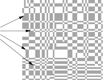
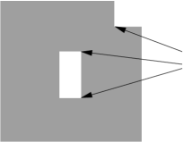
Figure 2: Typical states of the spin system above $T_{c}$ (left) and below $T_{c}$ (right). Some of the excited plaquettes are identified by arrows. They are ‘free’ above $T_{c}$, but ‘confined’ on corners of rectangular excitations in the ferromagnetic phase.

In the representation of figure 1, the concentration of vertices is given by $n_{p}$. The parameter $n_{b}$ is related to the total perimeter of the closed loops of that figure, and measures the spatial ordering of the vertices. The free plaquettes observed at $J=0$ have $n_{b}=(1/2)$. As $n_{b}$ is reduced, the reduction in the loop perimeter starts to constrain the positions of the vertices, and spatial correlations appear.

The internal energy per site is given by

$$\langle H/N\rangle=2Dn_{p}+4Jn_{b}-(D+2J)$$ (8)

so we have $n_{p}=(1+\partial f/\partial D)/2$ and $n_{b}=(2+\partial f/\partial J)/4$. Using (5), the paramagnetic state has

$$n_{p} \simeq [1+e^{2D/T}\cosh(2J/T)]^{-1}$$ (9)

$$n_{b} \simeq (1/2)-\frac{\sinh(2J/T)}{\cosh(2J/T)+e^{-2D/T}}$$ (10)

We see that introducing $J$ leads to small negative corrections to the $J=0$ values of $n_{p}$ and $n_{b}$. However, for $T<D$, the concentration of excited plaquettes is still approximately $c=e^{-2D/T}$ and these plaquettes are only weakly interacting since $n_{b}\simeq(1/2)$. A typical configuration is shown in figure 2: there are no two point correlations between the spins, but the loop vertices are dilute since $T\ll D$.

We now consider the system at temperatures lower than $T_{c}$. As shown in appendix A, a good approximation to the free energy per site in the ferromagnetic phase is

$$f_{\mathrm{fm}}^{(0)}=-D-2J-\frac{Te^{-8D/T}}{16\sinh^{2}(2J/T)}$$ (11)

which is valid for $J<T<T_{c}<D$. In this regime

$$n_{p} = \frac{e^{-8D/T}}{4\sinh^{2}(2J/T)}$$ (12)

$$n_{b} = \frac{e^{-8D/T}}{16\sinh^{2}(2J/T)\tanh(2J/T)}$$ (13)

For excitations in a ferromagnetic background, $n_{b}$ is directly related to the perimeter of the closed loops shown in figure 1. Equations (12) and (13) are therefore consistent with rectangular excitation loops with an excited plaquette at each corner (total energy cost $8D$). The expectation of the loop perimeter is approximately $(T/2J)$. This is much smaller than the typical spacing between loops, given by $(8J/T)e^{4D/T}$. This situation is sketched in figure 2.

The density of loops is given by the number of ways of forming such a loop, multiplied by a Boltzmann factor, $e^{-8D/T}$. We therefore identify the entropy per loop as $S_{\mathrm{loop}}\sim-2\log[4\sinh(2J/T)]$. The apparent divergence of the perimeter (and therefore the entropy) at small $J$ represents the breakdown of the ordered state which happens at $T_{c}$. The transition to the paramagnetic state occurs when the energy cost for adding two vertices to the loop ($4D$) is balanced by the entropy gain associated with adding an extra rectangular segment to the loop. This entropy gain is approximately $S_{\mathrm{loop}}$. We may therefore obtain an estimate of the transition temperature by setting $4D/T_{c}=S_{\mathrm{loop}}$. The result is

$$4\sinh(2J/T_{c})\simeq\exp(-2D/T_{c})$$ (14)

which differs from the exact result (2) only by the constant leading factor of 4. The real transition temperature is lower than that predicted by this method because interactions between the loops act to reduce the energies at large perimeters.

Thus we interpret the transition to the paramagnet as deconfinement of localised composite excitations. The state becomes disordered when the loop size becomes comparable with the spacing between loops.

The magnetisation and correlation lengths may also be calculated in similar series (see appendix A). The magnetisation, $M_{0}$, may be used to calculate the fraction of spins opposed to the mean spin,

$$n_{s}=\frac{1-M_{0}}{2}=\frac{e^{-8D/T}}{256\sinh^{4}(2J/T)}$$ (15)

Assuming that the lowest-lying excitations are rectangular domains with four excited plaquettes per domain, we expect a relation of the form $n_{s}=(n_{p}/4)(n_{b}/n_{p})^{2}$. We see that this is true for small $J/T$ [recall that $(J/T)$ is a small number, although expansions about $J=0$ are not valid in general since we are in an ordered phase].

Thus we have arrived at the following picture of the thermodynamics of the SEV model. There is a density of excited plaquettes $n_{p}$, which sit on the corners of overlapping closed loops. The total loop perimeter is measured in terms of the parameter $n_{b}$: the point $n_{b}=(1/2)$ is the maximally disordered spin field, in which the excited plaquettes are free. Away from the critical region (which is narrow), the excited plaquettes are nearly free in the paramagnetic phase: in the ferromagnetic phase then they are confined on corners of rectangular loops whose typical size is much smaller than their inverse density.

So far, our microscopic arguments have been purely thermodynamic: we have not considered any dynamics. In the next section, we investigate the dynamics of the SEV model.

III Dynamics

This section contains the key results of this paper. We briefly describe the dynamics of the paramagnetic state, which are essentially independent of $J$. We then discuss the onset of ordering as the temperature is lowered through $T_{c}$. We will find that supercooled states exist near $T_{c}$, which are well described by a simple ‘mobility field’ picture for times shorter than their lifetime. We then discuss the extent to which these states can be regarded as metastable, and what determines their lifetimes.

We begin with a very brief review of the dynamics in the paramagnetic state with $T<T_{o}$. Since $J$ may be treated perturbatively in this regime, we write the Hamiltonian as in equation (3). Flipping a single spin involves flipping of the four plaquette variables adjacent to that spin. Thus spins adjacent to four unexcited plaquettes have a flipping rate that is suppressed by a factor $e^{-8D/T}$. However, the flip rate of spins adjacent to exactly one excited plaquette are suppressed only by a factor $e^{-4D/T}$. The excited plaquettes mark mobile regions in which spin flips are rather likely. Thus the model resembles kinetically constrained systems such as the FA modelFAModel .

The relaxation time of the spins depends on the temperature and on the density of excited plaquettes, according to $\tau\sim n_{p}^{-1}e^{4D/T}$. This arises from localised one-dimensional diffusion of pairs of excited plaquettesBuhot2002 ; Espriu2003cm . In equilibrium, we have $n_{p}\simeq c=e^{-2D/T}$, so the relaxation time diverges as $c^{-3}$. More precisely, we have the scaling relationBuhot2002

$$\langle\sigma_{ij}(t_{w})\sigma_{ij}(t+t_{w})\rangle_{c,\mathrm{eq}}=f(c^{3}t)$$ (16)

for the on-site autocorrelation function in equilibrium at a given value of $c$. This is strong glass behaviour in the classification of Angell Angell .

We now turn to results for the SEV model below $T_{c}$, where $J$ may not be treated perturbatively. We discuss the phenomenological similarities and differences between this model and physical glass formers. We then interpret this behaviour with the aid of mean field rate equations.

III.1 Existence of supercooled states

Figure 3: Behaviour of the system after two quenches from infinite temperature to just below and just above $T_{c}=0.45D$. The two plateaux correspond to the onset of activated dynamics, and equilibration in the disordered (glassy) state. However, the disordered state is unstable below $T_{c}$, as is clear at longer times.

We start this section by demonstrating how a supercooled state may be formed below $T_{c}$. We investigate the dynamics of the system by means of simulations which use a continuous time Monte Carlo algorithmNewman-Barkema , with periodic boundary conditions. The number of excited plaquettes in each row and column is constrained to be even in this treatment, so the linear size of the system must be greater than $(2/n_{p})$ for reliable results. Some of the main features of the dynamics of the SEV model are shown in figure 3. We measure the energy density of the system with respect to the ground state:

$$u=\langle H/N\rangle+D+2J$$ (17)

The dashed trace in figure 3 shows the internal energy density after quenching to a temperature, $T_{1}$, such that $T_{c}<T_{1}<D$. After an initial transient, the system ages in a power law fashion towards equilibration at $u\sim 2De^{-2D/T_{1}}+2J$. The plateau at $(u/D)\simeq 0.2$ is a characteristic feature of models with kinetic constraints (whether explicitFAModel or emergentGarrahan-Newman ; Davison ). It represents the onset of ‘activated’ dynamics. The equilibration time for the paramagnet scales as a power of $c=e^{-2D/T}$. All these features are seen in the model with $J=0$ Lipowski ; barca .

In contrast, the full trace in figure 3 shows the behaviour on quenching to a temperature $T_{2}$ satisfying $T_{2}<T_{c}<D$, but with $T_{2}$ close to $T_{c}$. The behaviour resembles that of the quench to $T_{1}$, including apparent equilibration at $u\sim 2De^{-2D/T_{2}}+2J$. However, this is state is not stable, and the energy falls further at longer times. This behaviour resembles that of glass-formers, where the state on the lower plateau would be called a supercooled liquid. The behaviour is also qualitatively similar to that observed in Cavagna2003 .

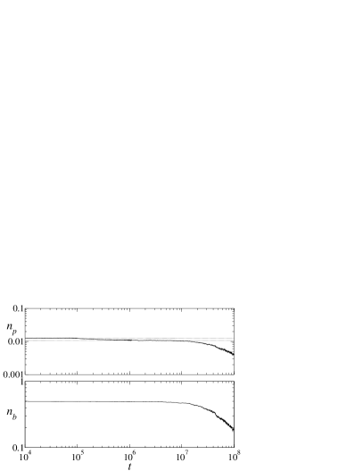
Figure 4: Behaviour of the SEV model after a quench from $T_{1}=1.02T_{c}$ to $T_{2}=0.996T_{c}$ with $T_{c}=0.45D$. We show concentrations of excited plaquettes, $n_{p}$, and broken bonds, $n_{b}$. The dotted lines mark $c_{1,2}=e^{-2D/T_{1,2}}$.

In order to focus on the supercooled states, we show further simulations in figure 4. The system is cooled through $T_{c}$ in a single small step. We plot $n_{p}$ and $n_{b}$ as a function of time. From the plot of $n_{p}$, we see that the density of free excitations responds relatively quickly to the change in temperature: it falls from $c_{1}=e^{-2D/T_{1}}$ to $c_{2}=e^{-2D/T_{2}}$, where it appears to stabilise.

The response of $n_{b}$ to the cooling is much slower. Recall that this correlation function measures the clustering of excited plaquettes. This clustering is a much slower process than the creation and annihilation steps leading to a change in the concentration of excitations. Looking at the late times in figure 4 when the clustering does start to occur, the system ages towards the ferromagnetic state with both $n_{p}$ and $n_{b}$ falling together. Taking the two traces in figure 4 together, we see that there are two separate timescales: one is associated with changes in $n_{p}$; the other with changes in $n_{b}$.

Turning to the supercooled state itself, it is clear from figure 4 that it has $n_{p}\simeq c=e^{-2D/T}$ and $n_{b}\simeq(1/2)$. This resembles closely the state that would be formed if we set $J=0$ in the Hamiltonian. Thus the effect of the interactions between plaquettes (the term proportional to $J$ in the Hamiltonian) is to set the lifetime of the supercooled state. The properties of the state itself are independent of $J$. We conclude that the supercooled state in the SEV model can be well described by the much simpler plaquette model of equation (3): a kinetically frustrated model with trivial thermodynamic properties. This is the assumption made when describing glass-formers by simple models of dynamical heterogeneityGCTheory ; Berthier2003 : in the SEV model, this assumption seems to be reasonable.

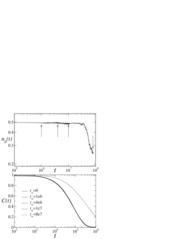
Figure 5: (Top) fraction of broken bonds against waiting time in the supercooled state: $T=0.996T_{c}$, $T_{c}=0.444D$. (Bottom) Autocorrelation function $C(t)=\langle\sigma_{ij}(t+t_{w})\sigma_{ij}(t_{w})\rangle$ for the waiting times marked in the top figure. The two-time function appears stationary until the system starts to nucleate at around $3\times 10^{7}$ Monte Carlo sweeps.

A key property of supercooled states is that two-time correlation functions should be stationary within the supercooled state. That is, expectation values of the form $\langle A(t_{w})A(t+t_{w})\rangle$ should be independent of $t_{w}$ as long as $(t+t_{w})$ is less than the lifetime of the states. In figure 5, we show that the supercooled state with $n_{p}=c$ and $n_{b}=(1/2)$ has this property. Since the excited plaquettes are uncorrelated in this state, it may be prepared manually, without the need for simulation. Further, the single spin autocorrelation function in the supercooled state is the same as that in the model with $J=0$ at the same temperature. It therefore obeys the dynamical scaling law of equation (16), and is independent of $J$.

As a final comment on figure 5, we note that the criterion that the supercooled state should be long-lived is fulfilled, since stationarity holds over timescales much longer than the single-spin relaxation time. Thus the data in that figure is consistent with the picture of a supercooled state that appears to equilibrate in a metastable basin.

III.2 Lifetime of supercooled states

Figure 6: Nucleation times at $T_{c}=0.50D$ and $T_{c}=0.44D$, measured by averaging over several runs similar to those in figure 5. The temperature increases from left to right, but note that the zero of the logarithmic scale is at $T_{c}$, away to the right. The dashed lines are fits to the form of equation (18) using the same value of $\gamma=0.17$. This form captures the qualitative features of the curve: a power law increase near $T_{c}$, and an exponential divergence at low temperatures.

Having identified a supercooled state at temperatures near $T_{c}$, we now proceed to discuss its lifetime. We prepared states with $n_{p}=c$ and $n_{b}=(1/2)$ and measured the time taken for $n_{b}$ to fall to $0.45$. Results are shown in figure 6. The lifetime gets very large both near $T_{c}$, and in the limit $T\to 0$.

Near $T_{c}$, the states are supercooled. At very low temperatures, the lifetimes are similarly long, but in this case they are of the same order as the spin relaxation time. These states are not equilibrated in a metastable basin; rather, their long lifetimes reflect the drastic slowing down of all timescales as the temperature is reduced.

From figure 6, we conjecture that the nucleation time has the form

$$\tau_{\mathrm{nuc}}=\gamma e^{2D/T_{c}}\frac{e^{4D/T}}{1-(T/T_{c})}$$ (18)

where $\gamma$ is a (microscopic) rate that depends only weakly on $T$ and $T_{c}$. Physically, the nucleation rate is suppressed by a Boltzmann factor that arises from the activated dynamics, and by a factor of $\Delta\mu/T\simeq(T_{c}/T)-1$, where $\Delta\mu$ is the free energy difference between ordered and disordered phases.

In other words, behaviour near $T_{c}$ is characterised by a separation of the nucleation time from the relaxation time, $\tau$. The minimum in the nucleation time occurs at

$$T_{x}=T_{c}[1-(T_{c}/4D)+\mathcal{O}(T_{c}/D)^{2}]$$ (19)

The relaxation time in the paramagnet given approximately by $\tau=0.14e^{6D/T}$, so at the minimum we have $\tau^{*}\simeq 0.14e^{(6D/T_{c})+(3/2)}$ and $\tau_{\mathrm{nuc}}^{*}\simeq 0.17(4D/T_{c})e^{(6D/T_{c})+1}$. The result is that $\tau_{\mathrm{nuc}}^{*}>\tau^{*}$ as long as $T_{c}<T_{o}\sim D$, which is the regime of interest in this section. The two timescales are well separated for all temperatures between $T_{x}$ and $T_{c}$.

This separation results from the small amount of free energy that is released on ordering. States in which these times are well-separated are ‘supercooled’, in the sense that the degrees of freedom associated with the relaxation time appear to equilibrate in a state that is known to be unstable at long times.

At very low temperatures, we see that $\tau_{\mathrm{nuc}}$ will become smaller than the extrapolated relaxation time $\tau_{J=0}\sim e^{6D/T}$. The result is that the physical relaxation time at low temperatures is smaller than $e^{6D/T}$. The dynamics of the aging state are faster than those of a similar state with $J=0$.

These results may be interpreted in the picture of the model as a combination of a zero temperature dynamical fixed point and a finite temperature thermodynamic singularity. The spin relaxation time is controlled by the activated dynamics associated with the zero temperature fixed point. It is large compared to microscopic timescales, but small compared to the lifetime of the supercooled state. That lifetime is very long near the thermodynamic transition: the slowing down is due to the small free energy difference between paramagnetic and ferromagnetic states. We comment here that ‘soft modes’ at large lengthscales are not relevant to the behaviour observed in simulations, due to the narrowness of the critical region.

While supercooled states are familiar in systems with first order phase transitions, they are not usually observed near second order transitions, such as the one discussed in this work. In first order systems, the nucleation time may be predicted by thermodynamic arguments. The free energy of a ($d$-dimensional) droplet of ordered phase in a disordered background is approximately $\sigma r^{d-1}-\Delta\mu r^{d}$ where $r$ is the linear size of the droplet, $\sigma$ the surface tension and $\Delta\mu$ is the free energy difference between the two phases. Thus, nucleation requires the formation of a droplet of linear size $r^{*}\sim\sigma/\Delta\mu$, with an associated free energy barrier proportional to $\Delta\mu^{-1}$ (in two dimensions). The nucleation rate is therefore suppressed by a factor $e^{-\sigma^{2}/T\Delta\mu}$. This is exponential suppression of nucleation.

From (18), we see that the SEV model has linear suppression: the nucleation rate is proportional to $\Delta\mu$. This second order system has weaker suppression than that predicted for first order systems. Since the transition in the SEV model is second order, there are processes by which the bulk of the system may be continuously changed from paramagnet to ferromagnet, without a large free energy barrier. These processes are slow because they require co-operative motion of many spins, but the exponential slowdown that would result from a high energy intermediate state is not observed. While the phenomenology of the SEV model resembles that of first order systems, the lifetimes of supercooled states tend to be shorter than those in systems with diverging free energy barriers near $T_{c}$. In this respect, the SEV model is an imperfect model of a glass-former. However, we argue that the free energy barrier between ordered and disordered states in first order systems should mean that the supercooled states are less affected by the critical point than those of the SEV model. Thus, if the thermodynamic singularity is largely irrelevant in this model, then we expect it to be even less relevant in similar first order systems.

III.3 Rate equation approach and aging behaviour

In order to understand the results of the previous section, we give a brief discussion of the aging behaviour of the system. We parameterise this behaviour in terms of mean-field rate equations for the observables $n_{p}$ and $n_{b}$. This will provide further evidence that the supercooled states are characterised by fast dynamics for the concentration of excited plaquettes, $n_{p}$, combined with much slower dynamics for their spatial ordering (measured by $n_{b}$).

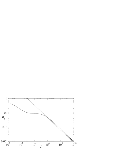
Figure 7: Plot showing aging of the paramagnet. We plot $n_{p}$ as a function of time after a quench from infinite temperature to $T=0.286D$, with $J=0$. The dashed line is a guide to the eye, corresponding to a decay proportional to $t^{-0.45}$.

In paramagnetic states with $T<D$, the equilibrium value of $n_{b}$ is $0.5$ and that of $n_{p}$ is $c\simeq e^{-2D/T}$. Aging towards equilibrium occurs at $n_{b}=0.5$, with $n_{p}\sim t^{-0.45}$ (a sample trace is shown in figure 7, but the observed exponent is independent of temperature, as long we work between $T_{c}$ and $T_{o}$). The rate is limited by the slow diffusion of excited plaquettes (there is no simple diffusive process for isolated excitations).

Figure 8: Aging of the system at a temperature $T=0.995T_{c}$. We have $T_{c}=0.451D$ so that $T>T_{x}$. We plot $n_{p}$ and $n_{p}/2n_{b}$ after a quench from infinite temperature. Both quantities are equal until the supercooled state becomes unstable. At these long times, $n_{p}$ decreases, but the ratio $n_{p}/2n_{b}$ remains constant with a value approximately equal to $c=e^{-2D/T}$.

There are two regimes for the aging towards the ferromagnetic state. We define $T_{x}$ as the temperature at which the nucleation time is minimal (recall figure 6). As shown in figure 3, after quenching to $T$ near $T_{c}$ ($T>T_{x}$), the system appears to equilibrate at $n_{p}=c$ (with $n_{b}=0.5$), before aging towards the ferromagnetic state. In figure 8 we show a similar scenario, but continuing to slightly longer times. At these long times, the system ages with the ratio $(n_{p}/2n_{b})\simeq c$. The decrease of $n_{b}$ happens on the long timescale given by $\tau_{\mathrm{nuc}}$. However, the plaquette concentration, $n_{p}$, is reacting on a much faster timescale. The interpretation is that $n_{p}$ has stabilised in an environment set by the current value of $n_{b}$. It seems that the stable value of $n_{p}$ is around $2cn_{b}$.

Figure 9: Aging at $T=0.364D$, with $T_{c}=0.444D$, so that $T<T_{x}$. The ratio $n_{p}/2n_{b}$ deviates from $n_{p}$ at a value around $e^{-2D/T_{c}}$, so the system does not reach the supercooled state with $n_{p}=c=e^{-2D/T}$.

If instead we quench to a temperature below $T_{x}$, there is no apparent equilibration at $n_{p}\simeq c$. Instead, the effect of finite $J$ becomes apparent when $n_{p}\simeq e^{-2D/T_{c}}>c$. There is a transient effect as $n_{b}$ begins to change, but the long time behaviour again has a constant ratio $(n_{p}/2n_{b})\simeq 0.8e^{-2D/T_{c}}$ (see figure 9). Simulations indicate that the constant value of $(n_{p}/2n_{b})$ seems to depend on $T_{c}$ as shown, and to vary only weakly with $T$. Further, the exponent associated with the aging appears to be similar to that in the paramagnetic state (around $0.45$). The natural interpretation is that the aging of these states is controlled in the same way as the aging of the paramagnet: by the slow diffusion of excited plaquettes. The dynamics of $n_{b}$ are now faster than those of $n_{p}$, and the spatial ordering of the excited plaquettes is responding faster than the plaquette density.

This description of the aging behaviour is consistent with the following conjectured rate equations

$$e^{4D/T}\partial_{t}n_{p} = \lambda_{p}n_{p}^{2.2}(2cn_{b}-n_{p})$$ (20)

$$e^{4D/T}e^{2D/T_{c}}\partial_{t}n_{b} = \lambda_{b}n_{b}[1-(T/T_{c})](X_{b}-2n_{b})$$

where $X_{b}=\mathrm{min}(1,n_{p}Ae^{2D/T_{c}})$. The significance of this quantity is that $n_{b}$ would equilibrate to $X_{b}/2$ if the concentration of plaquettes were constrained to be equal to $n_{p}$. The exponent $2.2$ in equation (20) is fixed by the exponent $0.45$ for the power law decay of the energy in the paramagnetic phase (as shown in figure 7). The the overall scaling of time with temperature in that equation is also fixed by the aging of the paramagnetic states. The scaling of time in (LABEL:equ:mf_nb) is determined by the scaling of the nucleation time in equation (18).

The adjustable parameters of the theory are therefore the rates $\lambda_{p}$ and $\lambda_{b}$, and the constant, $A$. The two rates are microscopic frequencies reflecting the co-operative motion of the spins required to change $n_{p}$ or $n_{b}$. The constant $A$ determines the ratio of $n_{b}$ and $n_{p}$ when the aging is controlled by plaquette diffusion (as in figure 9). The instability of the supercooled state means that $Ae^{2D/T_{c}}<e^{2D/T}$: the data of figure 9 is consistent with $(1/A)\simeq 0.8$, as mentioned above.

We make no attempt to justify these rate equations on microscopic grounds. For example, the exponent $2.2$ in equation (20) is a non-trivial decay exponent for an annihilation-diffusion problem in which diffusion of single excited plaquettes is suppressed by the kinetic constraint. We imagine ‘integrating out’ all the microscopic degrees of freedom: the effect of the complicated fluctuation effects appears only in this exponent. However, while their microscopic origin is unclear, the interesting feature of these equations are (1) the different temperature scaling of the times associated with the two degrees of freedom, and (2), the presence of points at which one degree of freedom is not changing. The first feature leads to a separation of timescales in the problem. When this is combined with the second feature, the apparent metastability of the supercooled states becomes possible. In this case, the faster degree of freedom is $n_{p}$, which equilibrates at $2cn_{b}$ on a timescale that is fast enough that $n_{b}$ can be considered to be constant. The aging of the supercooled state then has a timescale determined by the rate equation for $n_{b}$. That degree of freedom is trying to reach apparent equilibration at $n_{p}Ae^{2D/T_{c}}/2$, but $n_{p}$ is the faster degree of freedom, and is moving the target downwards just as fast as $n_{b}$ decreases towards it. This results in the aging at constant $n_{b}/n_{p}$ that is shown in figure 8. An exactly analogous process is taking place in figure 9, except that $n_{p}$ is now the slow degree of freedom.

The central point of the above argument is that the slow degrees of freedom set a ‘target value’ for the fast ones, at which the fast degrees of freedom appear to equilibrate when viewed on the fast timescale. This is the sense in which the states discussed in the previous section are ‘supercooled’. Their lifetime is then set by the slow degrees of freedom, and this lifetime is much longer than relaxation timescales in these states. To understand the correlations in the aging state, it would be desirable to study the thermodynamics of the excited plaquettes while working at fixed $n_{b}$. However, this is well beyond the scope of this paper.

Note that there is no provision in equations (20) and (LABEL:equ:mf_nb) for equilibration in a ferromagnetic state. However, the large internal energy difference between paramagnetic and ferromagnetic states means that this equilibration is not observed on timescales that are accessible in simulation. Therefore, equations (20) and (LABEL:equ:mf_nb) appear to be valid over timescales that are several orders of magnitude longer than the lifetimes of the supercooled states.

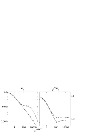
Figure 10: Fit to the data of figures 8 ($+$ symbols) and 9 ($\times$ symbols) using mean field rate equations (20,LABEL:equ:mf_nb). Note that the left and right panels each show data from two runs, showing how the different regimes are captured by the same rate equations. Parameters are $(\lambda_{p},\lambda_{b},A)=(350,17,0.85)$ for the data of figure 8, and $(\lambda_{p},\lambda_{b},A)=(350,17,1.20)$ for that of figure 9.

It is simple to verify that the qualitative behaviour of figures 4 and 7-9 may be fitted by equations (20) and (LABEL:equ:mf_nb), with appropriate values of $(\lambda_{p},\lambda_{b},A)$. See figure 10, in which we show reasonable agreement. Note however, that the onset of nucleation from the supercooled state is more sudden than that predicted by the mean field equations. The initial ordering is slower than the power law predicted by these simple rate equations.

The requirement of different parameters to fit the different simulations in figure 10 show the rather simplistic assumptions for the temperature scaling in the mean field equations. That is, the linear suppression of the nucleation rate with $(T_{c}-T)$ is valid only near $T_{c}$, necessitating adjustment of $\lambda_{b}$ at smaller temperatures. We have already commented that $A$ will be temperature dependent, but that this dependence has a weaker effect on $X_{b}$ than the exponential dependence of that quantity on $T_{c}$.

The fits of figure 10 using these mean field equations support our interpretation of figure 6 in terms of purely dynamical effects that do not depend on thermodynamic quantities like free energy barriers and spinodal points.

IV Discussion and Conclusions

We have shown that the SEV model can be interpreted in terms of a high temperature state in which excitations are free and point-like, and a low temperature phase in which these free excitations are confined into composite objects, with a characteristic size that is smaller than their spacing. The dynamics of the paramagnet are well described in a ‘mobility field’ picture similar to the FA model.

Near the transition to the ordered phase, ‘supercooled’ paramagnetic states have long lifetimes. Two-time correlation functions show stationarity in these states, and both their dynamics and their thermodynamics are well-described by the plaquette model. However, these states have finite lifetimes, beyond which stationarity is lost and it becomes clear that they are unstable to the ferromagnetic state. This situation resembles the situation in physical glass-formers, except that the presence of a first order transition in those systems means that the lifetimes of the supercooled states diverge much faster near $T_{c}$ than in the SEV model.

We have also shown that the mean field rate equations, (20) and (LABEL:equ:mf_nb), are a suitable framework for describing the out of equilibrium (aging) behaviour of the SEV model.

We end this work with some comments about the significance of these results in the context of the literature. Comparing with the work of Cavagna et al.Cavagna2003 , we note the similarity between the phenomenology of their model and the SEV model. However, the exact solution of the eight vertex model, and the understanding of the dynamics of the paramagnetic state that arises from previous work on the plaquette model allow us to investigate the behaviour from a more microscopic viewpoint.

We illustrate this with three points. Firstly, the internal energy of the SEV model changes very rapidly around $T_{c}$. From simulation evidence alone, we might (erroneously) conclude that the transition was first order. However, we know from theoretical considerations that the transition is second order. This knowledge is important when discussing the possible metastability of supercooled states. Secondly, the power law suppression of nucleation near $T_{c}$ in the SEV model results from the fact that our transition is second order. For a first order transition we would expect an exponential suppression. The nature of this suppression in Cavagna2003 does not seem to be clear. And finally, we are able to identify the minimum in figure 6 as arising not from the crossing of a spinodal, but rather from a crossover in timescales.

We would also like to point out some similarities between the paramagnetic phase of the SEV model and the models which are conjectured to be controlled by the behaviour of entropic droplets Xia-Wolynes ; Bouchaud2004cm . As mentioned above, the invariance of the Hamiltonian at $J=0$ under flipping a whole row or column of spins leads to a large (but non-extensive) ground state entropy. We have shown that the introduction of $J$ is largely irrelevant above $T_{c}$, and in the supercooled states. Therefore, we may interpret the low temperature paramagnetic states ($T_{c}<T\ll T_{o}$) as a ‘mosaic’ of the many $J=0$ ground states. The ‘droplets’ are referred to as ‘entropic’ in this scenario. This name arises because there does not seem to be an energetic argument for their stability, so it assumed that they are stabilised by some entropic mechanism. In the plaquette model, the borders between ‘droplets’ of each ground state are not one dimensional as one might expect, but rather arise from point-like excited plaquettes. This situation was alluded to in the recent paper of Bouchaud and BiroliBouchaud2004cm . Since there is no perimeter for a surface tension to couple to, the entropic forces are strong enough to stabilise the ‘mosaic’ state. This is the situation in the SEV model at finite $J$, but $T>T_{c}$.

If we accept the plaquette model as a realisation of the entropic droplet picture, it is interesting to note that the only fixed point in that model is at zero temperature. That is, although the entropy falls rapidly as the temperature is reduced through $T_{o}$, any extrapolation that leads to $S=0$ at a finite temperature is not valid. Rather, the entropy remains regular at all temperatures (even those in which the glassy phase is completely unstable to the crystal). In fact, $S_{\mathrm{glass}}>S_{\mathrm{crystal}}$ all the way down to $T=0$ (where $S_{\mathrm{glass}}$ is the entropy associated with the plaquette model and $S_{\mathrm{crystal}}$ is the entropy of the SEV model with the same value of $D$ and at the same temperature). In this scenario the Kauzmann paradox Angell is seen as arising from an unphysical linear extrapolation of the glassy entropy.

To conclude, we have shown that the plaquette model limit of the SEV model describes its behaviour in both stable and supercooled paramagnetic states. This model resembles both the mobility field description of glassy systems (as exemplified by the FA model) and the entropic droplet picture. However, there is no finite temperature fixed point in the theory of the glassy states; thus Kauzmann’s paradox is avoided. Taken together, these results are further evidence that theories without thermodynamic singularities at finite temperature are suitable for describing glassy states GCTheory ; Whitelam2004 ; Berthier2003 .

Appendix A Low and high temperature expansions of the eight vertex model

In this appendix, we consider the series for the free energy given by BaxterBaxterBook :

$$(f/T)=-\log c^{\prime}-\sum_{m}\frac{x^{m}((q/x^{2})^{m}-1)^{2}(1-x^{m})^{2}}{m(1-q^{2m})(1+x^{m/2})}$$ (22)

where $q$, $x^{2}$ and $c^{\prime}$ depend on the model parameters $(D/T)$ and $(J/T)$. The parameter $z$ in Baxter’s calculation is $1$ in the SEV model since the Hamiltonian is invariant under $90^{\circ}$ rotations. The dependence of $q$ and $x^{2}$ on the original parameters $(D,J)$ is rather indirect: the main task of this appendix will be to derive simple relations between $(q,x^{2})$ and $(D/T,J/T)$ in the ferromagnetic phase.

However, we first consider the contribution of the $\log c^{\prime}$ term to the free energy. In the paramagnetic phase we have

$$(f_{\mathrm{pm}}/T)\sim\log c^{\prime}=\log\left[e^{D/T}\cosh^{2J/T}+e^{-D/T}\right]$$ (23)

which is the result quoted as (5), and may be used to calculate properties of the paramagnetic phase. However, in the ferromagnetic phase we have $c^{\prime}=e^{(D+2J)/T}$, so taking only the leading term leads to the trivial result: $n_{p}=n_{b}=0$. There are no excitations in the ferromagnetic phase at this order. We must therefore estimate the parameters $x$ and $q$ in this phase.

The prescription for calculating these parameters is given by BaxterBaxterBook , but we give a brief review. The ratios $D/T$ and $J/T$ are used to calculate four parameters $(a,b,c,d)$. The partition function is symmetric under interchange of the four quantities $(a\pm b,c\pm d)$. We may therefore map the parameters into the principal regime, to give $(a^{\prime},b^{\prime},c^{\prime},d^{\prime})$ satisfying $c^{\prime}+d^{\prime}>c^{\prime}-d^{\prime}\geq a^{\prime}+b^{\prime}>a^{\prime}-b^{\prime}\geq 0$. These parameters are used to calculate $\Delta=(-(c^{\prime 2}+d^{\prime 2})+(a^{\prime 2}+b^{\prime 2}))/(2c^{\prime}d^{\prime}+2a^{\prime}b^{\prime})$ and $\gamma=(c^{\prime}d^{\prime}/a^{\prime}b^{\prime})$.

In the ferromagnetic phase we have $\gamma=\exp(4D/T)$. We work at $T_{c}<D$ so $\gamma$ is a very large number, and we arrive at

$$\Delta=\cosh(4J/T)[1-\gamma^{-1}(1+\frac{1}{\cosh(4J/T)})+\mathcal{O}(\gamma^{-2})]$$ (24)

The next step is to calculate the parameter $k$, from:

$$\gamma(1+k^{2})=\Delta^{2}(1+\gamma)^{2}-(1+\gamma^{2})$$ (25)

and the result is

$$k=\frac{e^{-4D/T}}{2\sinh^{2}(2J/T)[1+\cosh(2J/T)]}+\mathcal{O}(\gamma^{-2})$$ (26)

We have $0<k<1$, and $k$ is the elliptic modulus with nome $q$. That is,

$$-\log q\int_{0}^{1}\frac{\mathrm{d}t}{\sqrt{1-t^{2}}\sqrt{1-k^{2}t^{2}}}=\pi\int_{0}^{\infty}\frac{\mathrm{d}t}{\sqrt{1+t^{2}}\sqrt{k^{2}+t^{2}}}$$ (27)

For the series of (22) to converge quickly, we require $q<1$: in that case (27) reduces to $q\simeq(k^{2}/16)$, and therefore we have the approximate relation

$$q\simeq\frac{e^{-8D/T}}{128\sinh^{4}(2J/T)}$$ (28)

whose condition for validity is that $k$ be small, which requires that $\sinh(2J/T)\ll e^{-2D/T}$. This is the condition that we are well inside the ferromagnetic phase, as is clear from (2).

In order to evaluate the terms in (22), we also require an approximate form for $x$. The definition of $x$ is

$$\log\left(\frac{q}{x^{2}}\right)\int_{0}^{1}\frac{\mathrm{d}t}{\sqrt{1-t^{2}}\sqrt{1-k^{2}t^{2}}}=\int_{\sqrt{\gamma k}}^{\infty}\frac{\pi\,\mathrm{d}t}{\sqrt{1+t^{2}}\sqrt{k^{2}+t^{2}}}$$ (29)

from which the relation $x^{2}<q$ is clear. This integral may be expanded in a series around $(1/\sqrt{\gamma k})=0$. Equation (26) shows that this parameter is small if $J\ll T$. The result is that

$$(q/x^{2})-1\simeq 4\sinh(2J/T)$$ (30)

Substituting into (22), and ignoring all terms with $m\geq 2$, we arrive at

$$f_{\mathrm{fm}}\simeq-(D/T)-(J/T)-\frac{e^{-8D/T}}{16\sinh^{2}(2J/T)}$$ (31)

which gives the result (11), qualified by the validity condition

$$e^{-2D/T}\ll\sinh(2J/T)\ll 1$$ (32)

from which we note that this is not an expansion about $T=0$, but rather a useful approximation to the free energy in this part of the parameter space.

References

- (1) J. P. Garrahan and D. Chandler, Phys. Rev. Lett. 89, 035704 (2002); Proc. Natl. Acad. Sci. U.S.A. 100, 9710 (2003).
- (2) S. Whitelam, L. Berthier, and J. P. Garrahan, Phys. Rev. Lett 92, 185705 (2004).
- (3) L. Berthier and J. P. Garrahan, J. Chem. Phys. 119, 4367 (2003); Phys. Rev. E 68, 041201 (2003).
- (4) W. Götze and L. Sjögren, Rep. Prog. Phys. 55, 55 (1992).
- (5) G. Biroli and J.P. Bouchaud, Europhys. Lett. 67, 21 (2004).
- (6) D. Kivelson, S.A. Kivelson, X.L. Zhao, Z. Nussinov and G. Tarjus, Physica A 219, 27 (1995).
- (7) X. Xia and P.G. Wolynes, Proc. Natl. Acad. Sci. USA 97, 2990 (2000).
- (8) M. Mézard and G. Parisi, Phys. Rev. Lett. 82, 747 (1999); S. Franz and G. Parisi, J. Phys. C 12, 6335 (2000).
- (9) G. H. Fredrickson and H. C. Andersen, Phys. Rev. Lett 53, 1244 (1984).
- (10) Jäckle and Eisinger, Z. Phys. B 84, 115, (1991).
- (11) F. Ritort and P. Sollich, Adv. Phys. 52, 219 (2003).
- (12) A. Cavagna, I. Giardina and T. S. Grigera, Europhys. Lett. 61, 74 (2003); J. Chem. Phys. 118, 6974 (2003).
- (13) S. Franz, M. Mezard, F. Ricci-Tersenghi, M. Weigt and R. Zecchina, Europhys. Lett. 55, 465 (2001).
- (14) M. R. Swift, H. Bokil, R. D. M. Travasso and A. J. Bray, Phys. Rev. B 62, 11494 (2000).
- (15) A. Lipowski, J. Phys. A 30, 7365 (1997).
- (16) J.P. Garrahan and M.E.J. Newman, Phys. Rev. E 62, 7670 (2000).
- (17) J. P. Garrahan, J. Phys. Condens. Matter 14, 1571 (2002).
- (18) Y. Brumer, D.R. Reichman, Phys. Rev. E 69, 041202 (2004).
- (19) R. J. Baxter, Exactly solved models in statistical mechanics, (London : Academic Press, 1982).
- (20) A. Buhot and J. P. Garrahan, Phys. Rev. Lett 88, 225702 (2002).
- (21) D. Espriu and A. Prats, cond-mat/0312700.
- (22) C.A. Angell, Science 267, 1924 (1995).
- (23) M.E.J. Newman and G.T. Barkema, Monte Carlo Methods in Statistical Physics (Oxford University Press, Oxford, 1999).
- (24) L. Davison, D. Sherrington, J.P. Garrahan and A. Buhot, J. Phys. A 34, 5147 (2001).
- (25) J.-P. Bouchaud and G. Biroli, cond-mat/0406317.