Low-temperature internal friction and thermal conductivity in plastically deformed metals due to dislocation dipoles and random stresses

Abstract

The contribution to the low frequency internal friction and the thermal conductivity due to optically vibrating edge dislocation dipoles is calculated within the modified Granato-Lücke string model. The results are compared with the recent experiments on plastically deformed samples of Al, Ta and Nb at low temperatures. It is shown that the presence of a reasonable density of optically vibrating dislocation dipoles provides a good fit to the thermal conductivity in superconducting samples. At the same time, the internal friction experiments can not be described within the standard fluttering string mechanism. We found that the problem can be solved by assuming random forces acting on the dislocation dipoles. This gives an additional contribution to the internal friction which describes well the experimental data at low temperatures while their contribution to the thermal conductivity is found to be negligible.

I Introduction

Recently,Pohl:1999 ; Sahl:2001 ; Sahl2:2001 ; Sahl3:2002 ; Was:2002 the low-temperature internal friction, thermal conductivity, specific heat, and heat release of plastically deformed, high-purity superconducting crystalline samples of Al, Nb, and Ta have been experimentally studied and compared with measurements on amorphous SiO₂ specimen.Pohl:1999 ; Sahl:2001 ; Sahl2:2001 ; Sahl3:2002 In particular, it was established that plastic deformation has a pronounced effect on the internal friction and the thermal conductivity. Namely, the value of the internal friction can be increased by two orders of magnitude over that observed on annealed samples and it becomes comparable to that of amorphous SiO₂. Likewise, the thermal conductivity was found to have the similar value as that of amorphous SiO₂.Sahl:2001 ; Sahl2:2001 At the same time, neither long-time heat release nor additional contribution to the heat capacity expected for amorphous systems was observed. This finding indicates that the phonon scattering by dislocations appearing in crystals under plastic deformations could be of importance.

As is well known, there are two principal mechanisms of phonon scattering by dislocations: the static strain-field scattering and the reradiation scattering.Esh:1949 ; Nab:1951 The first one is due to the anharmonicity of the dislocation strain field while the second one results from a possibility of the sound wave to induce a dislocation vibration. In this case, the incident energy will be dissipated as long as the dislocation radiates elastic waves. This is so-called fluttering mechanism which is dynamical in its origin. It is a difficult problem to experimentally clarify what kind of scattering actually dominates and especially to obtain a quantitative agreement between the observed effect and theoretical calculations based on either static or dynamic models. Moreover, it was shown that both mechanisms of phonon scattering by an array of single dislocations are failed in the description of various experiments.Sahl:2001 ; Sahl2:2001 ; Sahl3:2002 ; Anderson:1972 ; Anderson:1979 For example, the estimated contribution to the thermal conductivity due to the resonant interaction was found to have a reasonable agreement with the experimental data only at very short lengths of dislocation lines (otherwise the resonant frequency becomes too low). Notice that a similar problem has already emerged in experiments with plastically deformed LiF.Anderson:1972 ; Anderson:1979 Namely, the measurements of the thermal conductivity and the ballistic phonon propagation in deformed LiF at low temperatures show that the obtained phonon scattering is too strong to be explained by static mechanisms of phonon-dislocation interaction, but is in rough agreement with calculations based on a resonant or dynamic interaction with dislocations which can flutter in the stress field of passing phonons. The crucial role in explanation of the experimental data plays an assumption given in Ref.Kneezel:1982, that a reasonable density of optically vibrating dislocation dipoles is present in LiF. In this case, the resonant frequency becomes markedly higher. It should be mentioned that dislocation dipoles with a rather high density were actually observed in LiF Gilman:1960 as well as in some other materials. For example, estimates from experiments of the ratio of the dislocation dipole density to a density of single dislocations range from $1000$ (in strain-hardening measurements Gilman:1960 ) to $100$ (by deformation-induced bulk-density changes Davidge:1964 ) and less (by electron microscopy Washburn:1966 ; Hesse:1972 ).

The purpose of this paper is to show that the concept of dynamical scattering of phonons by dislocation dipoles Kneezel:1982 previously used for the explanation of the experiments in LiF Anderson:1972 ; Anderson:1979 could also be suitable for Al, Nb, and Ta. As was observed in Refs.Sahl:2001, ; Sahl2:2001, ; Sahl3:2002, , these metals show a complex dislocation structure under plastic deformation. We assume that, by analogy with LiF, dislocation dipoles are also present in plastically deformed Al, Nb, and Ta. It should be noted that the dipole is a stable dislocation structure arising under plastic deformation in metals (see, e.g., Ref.Friedel:1964, ). Recently,Kassner:1999 ; Kassner:2000 the substructure of the dislocation ensemble in Al and Cu was experimentally studied under cyclic deformation. In particular, it was found in Ref.Kassner:1999, that for Al deformed at 77 K the microstructure is composed exclusively of vein dipole bundles and channels without persistent slip bands. The dislocation density in the veins is about $3.2\times 10^{14}$ m^-2, and the density in the channels is about $2.4\times 10^{13}$ m^-2 with the dipole separation in a range from 3 nm to 30 nm. It is important to note that all of the channel defects were found to be edge dipoles. In addition, the computer modelling performed in Ref.Aslanides:2000, shows that there is a critical size of the dipole separation (1.6 nm for Al and 0.42 nm for Cu) above which edge-dislocation dipoles in Al and Cu become stable with respect to the athermal annihilation. Notice that we consider in our paper dislocation dipoles in Al with a separation close to 20 nm, that is much larger the critical size found in Ref.Aslanides:2000, .

Thus, as for LiF the gain in resonant frequency can be achieved due to optically vibrating dipoles having a reasonable dipole separation and dislocation length. This allows us to obtain a quantitative agreement with the experimental data for all three metals. Evidently, the presence of the fluttering dislocation dipoles will affect not only the thermal conductivity but also other physical characteristics, in particular, the internal friction. We study the contribution to the internal friction due to vibrating dislocation dipoles in the framework of the modified Granato-Lücke string theory. As is known, the Granato-Lücke vibrating string model is based on an analogy between the vibration of a pinned dislocation line segment and the forced damped vibration of a string.Granato:1956

Our study shows that a good agreement with the internal friction experiments in Al, Nb, and Ta Pohl:1999 ; Sahl3:2002 ; Was:2002 can be obtained only in the presence of some random component of the stresses. This idea has been recently proposed and studied in Refs.Chernov:2002, and Kamaeva:2004, . In particular, it was found that the action of random forces on the dislocation gives a substantial contribution to the decrement. As was observed experimentally,Pohl:1999 ; Sahl3:2002 the decrement has an unexpectedly large value and practically does not depend on the amplitude and the frequency of external stresses. This means that the noise parameters should be governed by the characteristics of an external signal because this is the only way to provide the constant contribution to the decrement. Therefore, we suggest that the external force introduces also a specific time scale for correlations of stress fluctuations in dislocation ensemble which always has its own stochastic dynamics.Groma:1998 This time scale determines the time of an additional relaxation of internal stresses due to random stresses. It seems reasonable to assume that this time is related to the frequency of the external force. As the simplest approximation, we use the correlation function exponentially decreasing with time. What is important, the introduction of a time scale means that dislocations experience the influence of the colored noise. Finally, we adapt the theory proposed in Refs.Chernov:2002, and Kamaeva:2004, to the case of dislocation dipoles and introduce the additional noise component with the above-mentioned correlation function in the equations of motion.

II The model

Let us consider a dislocation dipole with dislocation lines directed along the z-axis and lying in parallel glide planes at distance $l$. The Burgers vectors are opposite while the orientation of dislocation lines is the same. The $xz$ plane is chosen to be a slip plane for a positive dislocation. In this case the plane $y=l$ is the slip plane for a negative dislocation. Within the string approximation, the dislocation dipole can be modeled by means of two damped interacting vibrating strings. Supposing that all the parameters of the string are the same for both dislocations, one can formulate the general equations of damped glide motion for the edge dislocation dipole in the form

$$m\frac{\partial^{2}\epsilon(z,t)}{\partial t^{2}}+B\frac{\partial\epsilon(z,t)}{\partial t}-T_{0}\frac{\partial^{2}\epsilon(z,t)}{\partial z^{2}}=F^{ext+},$$

$$m\frac{\partial^{2}\psi(z,t)}{\partial t^{2}}+B\frac{\partial\psi(z,t)}{\partial t}-T_{0}\frac{\partial^{2}\psi(z,t)}{\partial z^{2}}=F^{ext-},$$ (1)

where $\epsilon(z,t)$ and $\psi(z,t)$ are the displacements of the positive and negative dislocations, $m$ the effective mass, $T_{0}$ the line tension, $B$ the damping parameter, and $F^{ext\pm}$ the total external force which acts on the positive and negative dislocations, correspondingly, in their glide planes. The parameters of the model are written as Kneezel:1982

$$m=\frac{\rho b^{2}}{4\pi}[1+(c_{t}/c_{l})^{4}]\ln g,\qquad T_{0}=\frac{\mu b^{2}}{4\pi(1-\nu)}\ln g,\qquad B=\frac{\rho b^{2}\overline{\omega}}{8}[1+(c_{t}/c_{l})^{4}],$$ (2)

where $\rho$ is the density, $\mu$ the shear modulus, $\overline{\omega}$ the thermal phonon frequency, $\nu$ the Poisson constant, $b$ the length of Burgers vector, $c_{t}$ and $c_{l}$ the transverse and longitudinal sound velocities. At low frequencies, $g$ can be estimated as $g\sim 1/b\sqrt{\Lambda}$ where $\Lambda$ is the dislocation dipole density. The total external force, resolved in the glide plane, includes three terms

$$F^{ext\pm}=f^{\pm}+F^{\pm}+b^{\pm}\eta(t).$$ (3)

Here $f^{\pm}$ are the interaction forces between the dislocations in the dipole, $F^{\pm}$ are the forces due to external stress field $\sigma_{ik}$, and $\eta(t)$ describes a stationary random component. The explicit form of $\eta(t)$ is not specified at this stage. Hereafter, the sign plus (minus) corresponds to a positive (negative) dislocation, and the summation over repeated indices is assumed. In general, the interaction between dislocations is determined by the Peach-Koehler force

$$f^{\pm}_{j}=\varepsilon_{jak}\tau_{a}b_{i}^{\pm}\sigma^{\mp}_{ik},$$ (4)

where $\varepsilon_{jak}$ is the totally antisymmetric tensor, $\sigma^{\mp}_{ik}$ are the corresponding stresses of dislocations in the dipole, and $\vec{\tau}$ is the unit tangent vector to the defect line. The displacement fields can be written as

$$u_{n}\left(\vec{r},t\right)=\int c_{ijkl}G_{jn,i}\delta e^{pl}_{kl}dV^{{}^{\prime}},$$ (5)

with $c_{ijkl}$ being the elastic modulus, $G_{jn}$ the Green’s tensor, $G_{jn,i}=\partial G_{jn}/\partial x_{i}$, and $\delta e^{pl}_{kl}$ the variation of the plastic part of the strain tensor. For sliding dislocation one has Landau:1970

$$\delta e^{pl}_{kl}=\frac{1}{2}(b_{k}[\vec{\delta x}\vec{\tau}]_{l}+b_{l}[\vec{\delta x}\vec{\tau}]_{k})\delta(\vec{\xi}),$$ (6)

where $\vec{\delta x}$ describes the displacement of the dislocation line from a straight configuration and $\delta(\vec{\xi})$ is the two-dimensional delta-function. In our geometry, $\vec{b}^{+}=-\vec{b}^{-}=(b,0,0)$, $\vec{\tau}=(0,0,-1)$, $\vec{\xi}^{+}=(x^{\prime},y^{\prime},0)$, and $\vec{\xi}^{-}=(x^{\prime},y^{\prime}-l,0)$. The displacements are chosen to be $\vec{\delta x^{+}}=(\epsilon(z),0,0)$ and $\vec{\delta x^{-}}=(\psi(z),0,0)$, so that $[\vec{\delta x^{+}}\vec{\tau}]=(0,\epsilon,0)$ and $[{\vec{\delta}x^{-}}\vec{\tau}]=(0,\psi,0)$. After substitution into Eq.(5) one obtains

$$u^{+}_{n}(\vec{r})=\int c_{ijk2}G_{jn,i}(x,y,z-z^{\prime})b^{+}_{k}\epsilon(z^{\prime})dz^{\prime},$$

$$u^{-}_{n}(\vec{r})=\int c_{ijk2}G_{jn,i}(x,y-l,z-z^{\prime})b^{-}_{k}\psi(z^{\prime})dz^{\prime}.$$ (7)

For isotropic case,

$$G_{km}(\vec{r})=\frac{1}{8\pi\mu}\left[\frac{2}{r}\delta_{km}-\frac{1}{2(1-\nu)}r_{,km}\right]$$

and $c_{ijkl}=\lambda\delta_{ij}\delta_{kl}+\mu(\delta_{ik}\delta_{jl}+\delta_{il}\delta_{jk})$ with $\lambda$ and $\mu$ being the Lame constants. Supposing that $\epsilon(z)=\epsilon(k)\exp(ikz)$ and $\psi(z)=\psi(k)\exp(ikz)$, after straightforward calculations one obtains from Eq.(4)

$$f^{-}(\vec{r})=-2\epsilon(k)e^{ikz}\mu^{2}b^{2}k^{2}\Biggl{[}2A\left(1-\frac{8x^{2}y^{2}}{a^{4}}\right)K_{2}(ka)-\frac{4Akx^{2}y^{2}}{a^{3}}K_{1}(ka)+(2A+B)K_{0}(ka)\Biggr{]},$$ (8)

$$f^{+}(\vec{r}) = -2\psi(k)e^{ikz}\mu^{2}b^{2}k^{2}\Biggl{[}2A\left(1-\frac{8x^{2}(y-l)^{2}}{c^{4}}\right)K_{2}(kc)-\frac{4Akx^{2}(y-l)^{2}}{c^{3}}K_{1}(kc)+$$ (9)

$$+(2A+B)K_{0}(kc)\Biggr{]},$$

where $A=-B/4(1-\nu)$, $B=1/4\pi\mu$, $a^{2}=x^{2}+y^{2}$, $c^{2}=x^{2}+(y-l)^{2}$, and $K_{\nu}$ are the McDonalds functions. Notice that we are interested only in a component $f_{1}$ since, at chosen geometry, all the remaining components become equal to zero in slip planes of dislocations. In the long wavelength approximation ($kl\ll 1$) one gets

$$f^{-}(0,l,z)=D\epsilon(z),\quad f^{+}(0,0,z)=D\psi(z),$$ (10)

where

$$D=\frac{\mu b^{2}}{2\pi(1-\nu)l^{2}}.$$ (11)

The second term in Eq.(3) is also determined by the Peach-Koehler force which is written in the known form $F^{\pm}_{r}=\varepsilon_{rak}\tau_{a}b_{i}^{\pm}\sigma_{ik}$ with $\sigma_{ik}$ being an external stress field. In our geometry,

$$F^{+}=b^{+}\sigma(0,0,z),\quad F^{-}=b^{-}\sigma(0,l,z).$$ (12)

Let us consider first the case of free vibrations of the dipole when $B=F^{\pm}=\eta(t)=0$ in Eq.(II). There exist both acoustical and optical modes with $\epsilon=\psi$ and $\epsilon=-\psi$, respectively. Substituting Eq.(10) into Eq.(II) one obtains

$$m\frac{\partial^{2}\epsilon(z,t)}{\partial t^{2}}-T_{0}\frac{\partial^{2}\epsilon(z,t)}{\partial z^{2}}\pm D\epsilon(z)=0.$$ (13)

Here the sign plus corresponds to the optical mode while the minus to the acoustical one. The spectrum of normal oscillations is found to be

$$\Omega^{\pm}_{n}=\sqrt{\omega^{2}_{n}\pm\frac{D}{m}},$$ (14)

where $\omega_{n}=(\pi n/L)\sqrt{T_{0}/m}$ is the resonance frequency of a single dislocation and L is the dislocation length. For optical mode, this spectrum was presented in Ref. Kneezel:1982, . As is seen, the resonance frequency becomes higher for the optical mode and the difference increases with decreasing dipole separation. On the contrary, for acoustical mode the resonance frequency lies even lower than that for a single dislocation.

The measured thermal conductivity can be fitted by assuming dislocation dipoles having a higher resonant frequency and being more numerous than isolated dislocations. Kneezel:1982 For this reason, we consider below only the case of optically vibrating dislocation dipoles. Supposing $\epsilon=-\psi$, $\sigma(0,0,z)=\sigma(0,l,z)$, and taking into account Eqs.(3), (10) and (12) one can reduce Eq.(II) to

$$m\frac{\partial^{2}\epsilon(z,t)}{\partial t^{2}}=T_{0}\frac{\partial^{2}\epsilon(z,t)}{\partial z^{2}}-B\frac{\partial\epsilon(z,t)}{\partial t}+b\sigma(0,0,z)-D\epsilon(z,t)+b\eta(t).$$ (15)

Let us consider a periodic external stress wave in the form

$$\sigma(0,0,z)=\sigma_{0}e^{i\omega t}=\sum\limits_{n}\sigma_{n}\sin(k_{n}z)e^{i\omega t},$$ (16)

where $\sigma_{0}$ is the shear stress component resolved in the glide plane, $k_{n}=\pi n/L$, and $\sigma_{n}=4\sigma_{0}/\pi n$ is the Fourier coefficient. Then the general solution to Eq.(15) is written as

$$\epsilon(z,t)=\sum\limits^{\infty}_{n=1}\epsilon_{n}(t)\sin(\pi nz/L).$$ (17)

Besides, $\epsilon_{n}(t)$ can be presented as the sum of periodic and random components

$$\epsilon_{n}(t)=\epsilon_{n}(t)_{p}+\epsilon_{n}(t)_{r}.$$ (18)

Substitution of Eqs.(17) and (18) into Eq.(15) gives the following system of equations:

$$\frac{\partial^{2}\epsilon_{n}(t)_{r}}{\partial t^{2}}+\frac{B}{m}\frac{\partial\epsilon_{n}(t)_{r}}{\partial t}+\Omega^{+2}_{n}\epsilon_{n}(t)_{r}-\frac{4b\eta(t)}{\pi nm}=0,$$

$$\frac{\partial^{2}\epsilon_{n}(t)_{p}}{\partial t^{2}}+\frac{B}{m}\frac{\partial\epsilon_{n}(t)_{p}}{\partial t}+\Omega^{+2}_{n}\epsilon_{n}(t)_{p}-\frac{4b\sigma_{0}e^{i\omega t}}{\pi nm}=0.$$ (19)

The solution to the second equation is written as

$$\epsilon_{n}(t)_{p}=C_{n}e^{i\omega t},$$ (20)

with

$$C_{n}=\frac{b\sigma_{n}}{m}\frac{1}{\left(i\frac{B\omega}{m}+\Omega^{+2}_{n}-\omega^{2}\right)}.$$

The solution to the first equation in Eq.(II) is written in the form

$$\epsilon_{n}(t)_{r}=\frac{1}{m\sqrt{\Omega^{+2}_{n}-\frac{B^{2}}{4m^{2}}}}\int\limits_{0}^{t}\frac{4b\eta(\tau)}{\pi n}e^{-B(t-\tau)/2m}\sin\sqrt{\Omega^{+2}_{n}-\frac{B^{2}}{4m^{2}}}(t-\tau)d\tau.$$ (21)

As is seen, the displacement $\epsilon_{n}(z,t)$ depends on the random function $\eta(t)$. As a result, the dipole dynamics is governed by a random function having its own probabilistic characteristics. This is an essential difference from the standard string model where the string is subjected only to the influence of the periodic force.

III Internal friction

Let us calculate the total decrement $\Delta_{t}$ due to the motion of optically vibrating edge dislocation dipoles by using the formulated model. Since $\epsilon_{n}(t)$ is a random function, one has to perform an additional averaging over the possible realizations of random stresses $\eta(t)$. The mean energy loss to friction due to optically vibrating edge dislocation dipole per unit time reads

$$<\overline{P}>=2\int\limits_{0}^{L}\lim\limits_{T\rightarrow\infty}\frac{1}{T}<\int\limits_{0}^{T}(F^{+}+b\eta(t))\frac{{\partial\epsilon(z,t)}}{\partial t}dt>dz,$$ (22)

where $<>$ means averaging over random force realizations ensemble. Generally,

$$\Delta_{t}=\frac{<\Delta W>}{2<W>}=\frac{N<\Delta W_{d}>}{2<W>}=\frac{N<\overline{P}>}{2<W>}\frac{2\pi}{\omega},$$ (23)

where $<W>$ is the averaged total vibration energy per unit volume, N is the total number of dislocation dipoles per unit volume, $<\Delta W_{d}>$ is the contribution from the single dislocation dipole. After substitution of Eq.(18) into Eq.(22) the decrement is written as

$$\Delta_{t}=\Delta_{r}+\Delta_{p},$$ (24)

where

$$\Delta_{r}=\lim\limits_{T\rightarrow\infty}\sum\limits_{l=0}^{\infty}\frac{16J}{m\omega\pi(2l+1)^{2}}\int\limits_{0}^{T}<\eta(T-S)\eta(T)>e^{-BS/2m}\left(\cos(\Omega_{l}S)-\frac{B}{2m}\frac{\sin(\Omega_{l}S)}{\Omega_{l}}\right)dS,$$

$$\Delta_{p}=\sum\limits_{p=0}^{\infty}\frac{8JB\sigma^{2}_{0}\omega}{\pi E_{p}(2p+1)^{2}},\quad E_{p}=\left(D-m\omega^{2}+\frac{T_{0}\pi^{2}}{L^{2}}\left(2p+1\right)^{2}\right)^{2}+B^{2}\omega^{2},\quad J=\frac{b^{2}LN}{<W>}=\frac{b^{2}\Lambda}{2<W>}.$$

Eq.(24) describes the contribution to the internal friction due to dislocation dipoles under the action of both periodic and random forces. As is known, the decrement describes how quickly the amplitude of a wave decays. In turn, the scattering rate, which is necessary to describe the thermal conductivity, defines the rate at which the incident wave loses its energy to the dislocation dipoles. It is given by

$$\tau^{-1}_{d}=\frac{\Delta_{t}\omega}{\pi}.$$ (25)

Notice that both the decrement and the scattering rate depend on two sets of parameters. The first one (T₀, B, m, D) characterizes the string and can be calculated from Eqs. (2) and (11). The second set comes from the characteristics of the dipole’s ensemble such as the density of dipoles $\Lambda$ and the correlation function $<\eta(T-S)\eta(T)>$. In general, the dislocation density depends on the plastic deformation in a sample. Typically, a phenomenological relation between the plastic strain $\epsilon$ and the dislocation density is used. Experimentally the plastically deformed samples of Al, Ta, and Nb were studied. Pohl:1999 ; Sahl:2001 ; Sahl2:2001 ; Sahl3:2002 ; Was:2002 The densities of dislocations in these materials depend on the specimen preparation and vary in the range $10^{13}-4\times 10^{14}$ m^-2.Pohl:1999 ; Sahl:2001 ; Sahl2:2001 ; Sahl3:2002 ; Was:2002 In our calculations we try to choose such dipole densities which give the best fit.

As was mentioned in the introduction, we assume that the stochastic stress component appears naturally in a high-density dislocation arrangement. Let us discuss this point in more detail. Evidently, it is impossible to describe the exact dynamical behavior of large dislocation ensemble in the complex potential relief. Instead, one can use the statistical consideration by introducing the statistical fluctuations of stresses. Notice that even idealized numerical simulations of the overdamped dynamics of an array of parallel edge dislocations with long-range interactions in Ref. Groma:1998, show an appearance in this system of the stochastic component of the internal stress field. According to Ref. Groma:1998, , for a period of time shorter than the relaxation time of the dislocation system, the internal stresses caused by dislocations in the arrangement can be viewed as a sum of slowly varying mean stress originating from the internal stress of the smoothed out dislocation distribution and a rapidly varying, highly irregular function with a zero mean value that satisfies the requirement of no correlation at different times or places and that represents the influence of the nearest neighbors. In this case, the stochastic stress component has a white noise character.

Our calculations show that the white noise does not give a contribution to the internal friction. As is well known, however, the white noise concept does not reflect the real physical processes in complex systems. A possible way to generalize the consideration is to introduce the colored noise which can be modeled by exponentially decreasing correlator in the simplest case. As possible sources of colored noise in dislocation ensemble one can mention an external force, a long-range interaction between dislocations, the lattice itself, etc. Actually, we consider the dichotomic noise which is characterized by

$$<\eta(t)>=0,\quad<\eta(t_{1})\eta(t_{2})>=\eta_{0}^{2}e^{-2\alpha\mid t_{1}-t_{2}\mid},$$ (26)

where $\alpha$ is a parameter of the corresponding Poisson process, $\eta_{0}^{2}$ the dispersion. Taking into account Eqs.(24) and (26), as well as the fact that for dichotomic noise $<W>=(\eta^{2}_{0}+\sigma^{2}_{0}/2)/2\mu$, the total decrement reads

$$\Delta_{t}=\frac{4\pi J\eta^{2}_{0}}{(4\alpha^{2}m+2\alpha B+D)}\left[1-\tanh(Y_{t})/Y_{t}\right]\frac{\alpha}{\omega}+\sum\limits_{p=0}^{\infty}\frac{8JB\sigma^{2}_{0}\omega}{\pi E_{p}(2p+1)^{2}},$$ (27)

with

$$Y_{t}=\frac{\pi}{2}\sqrt{\frac{(4\alpha^{2}m+2\alpha B+D)}{T_{0}(\pi/L)^{2}}}.$$

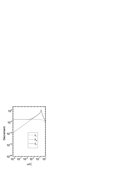
Figure 1: The calculated internal friction using the parameter set for the 10% deformed high purity 5N polycrystalline aluminium sample (Tables I and II) and $\Omega^{+}_{1}=10^{11}$ Hz.

Fig.1 shows the decrement given by Eq.(27) as a function of the reduced frequency for parameters of polycrystalline Al. The corresponding material constants for Al, Ta and Nb are presented in Table 1. As is seen from Fig.1, at low frequencies (up to 10⁸ Hz) the total decrement is a constant. It is important to note that such behavior is entirely determined by the contribution from the random part of stresses. The situation changes drastically near the resonance frequency where the decrement has a sharp peak and mainly depends on losses due to the periodic external stresses. Namely, $\Delta_{p}$ is found to be $10^{4}$ larger than $\Delta_{r}$ near the resonance frequency. Notice that a similar behavior is also found for both Ta and Nb. In experiments, Pohl:1999 ; Sahl3:2002 ; Was:2002 the low-frequency (90kHz Pohl:1999 ; Sahl3:2002 and 1kHz Was:2002 ) internal friction was studied. Therefore, the region of the constant decrement is of our main interest here. In addition, in our model the following condition is fulfilled

$$D\gg T_{0}\pi^{2}/L^{2}.$$ (28)

This is a variant of the so-called ”rigid” relief approximation. Kamaeva:2004 Moreover, a reasonable restriction on the dispersion of colored noise can be imposed in the form $\eta^{2}_{0}/\sigma^{2}_{0}\ll 1$. In view of Eq.(28), performing the summation in Eq.(27) one finally obtains

$$\Delta_{t}=\frac{8\pi\mu b^{2}\Lambda}{D}\frac{\eta^{2}_{0}}{\sigma^{2}_{0}}\frac{\alpha}{\omega}+\frac{2\pi\mu\Lambda Bb^{2}\omega}{D^{2}}.$$ (29)

The decrement given by Eq.(29) for different specimens is presented in Table 2. As is seen, there is a good agreement with the experimental data Pohl:1999 ; Sahl3:2002 ; Was:2002 at appropriate choice of the model parameters. Notice that only two arbitrary model parameters ($\alpha/\omega$ and $\eta^{2}_{0}/\sigma^{2}_{0}$) were used in our calculations.

It was observed in experiments Pohl:1999 ; Sahl3:2002 ; Was:2002 that the low-frequency internal friction does not depend on either the temperature or the frequency at low temperatures. In the framework of our model this behavior can be explained only when both the interaction between dislocations (in a dipole) and the colored noise are present. Namely, the colored noise gives a dominant contribution (in comparison with the Granato-Lucke mechanism) to the decrement at low frequencies. At the same time, the athermal long-distance interaction (determined completely by the structure of the dislocation ensemble) provides the athermal behavior of the low-frequency internal friction at low temperatures. Indeed, this interaction ensures the validity of the ”rigid” relief approximation (see Eq.(28)) when both the temperature-dependent terms (containing the damping parameter $B$) and the terms containing the tension and the mass of the string are negligible in Eq.(27). Let us note that a similar role of the long-range interactions was earlier discussed in Ref. Kustov:1999, in a study of solid solutions. In particular, it was shown that the long-range interaction of dislocations with solute atoms distributed in the bulk of the crystal supports the athermal behavior of the nonlinear dislocation strain-amplitude-dependent internal friction in solid solutions. Kustov:1999 ; Gremaud:2004

We also assume the linear response of the dislocation array to the external periodic forces which means $\alpha/\omega$=const, $\eta^{2}_{0}/\sigma^{2}_{0}$=const. Without loss of generality one can fix the first constant as unity at numerical evaluations. Notice that, strongly speaking, these assumptions do not provide the independence of the decrement from frequency. Actually, this is true only for low-frequency asymptotic of the contribution to the decrement from random forces. Indeed, as is seen from Fig.1 the decrement $\Delta_{r}$ decreases rapidly at high frequencies.

IV Thermal conductivity

As is well-known, at low temperatures the main contributions to the thermal conductivity come from the lattice defects and boundary scattering. Within the framework of the relaxation time description and the Debye approximation the lattice thermal conductivity is given by

$$\kappa=\sum\limits_{j=1}^{3}(1/6\pi^{2}v_{j})\int\limits_{0}^{\omega_{Dj}}\tau_{j}(\overline{\omega}_{j})\overline{\omega}^{2}_{j}C_{j}(\overline{\omega}_{j})d\overline{\omega}_{j},$$ (30)

where the sum includes the longitudinal and two transverse acoustical phonon modes. $\omega_{Dj}$ is the Debye frequency, $v_{j}$ the sound velocity, $\tau_{j}$ the total phonon relaxation time and $C_{j}$ the specific heat of the phonon mode $j$. Assuming that all phonon modes are scattered almost equally by the dislocation dipoles, the total relaxation rate $\tau^{-1}$ is written as

$$\tau^{-1}=\tau^{-1}_{c}+\tau^{-1}_{d},$$ (31)

where $\tau^{-1}_{c}$ is the relaxation rate of the boundary scattering, and $\tau^{-1}_{d}$ is the relaxation rate due to the dynamic phonon-dipole interaction. As another approximation, we will use the averaged sound velocity $\overline{v}$ instead of sound velocity of the phonon mode $j$. In other words, we drop the polarization effects. It is also convenient to use the dimensionless variable $x=\hbar\overline{\omega}/kT$ so that Eq.(30) takes the form

$$\kappa=(k^{3}/2\pi^{2}\overline{v}\hbar^{3})T^{3}\int\limits_{0}^{\theta/T}x^{2}\tau(x)C(x)dx,$$ (32)

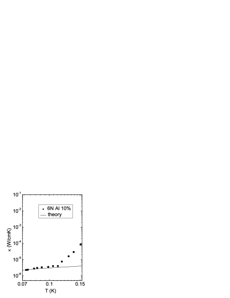
Figure 2: Thermal conductivity for Al. Experimental data denoted by squares are from Ref. 3. The solid line represents the theoretical curve for $\Lambda_{Al}=6\times 10^{12}$ m^-2 using the parameter set from Table I. The resonance frequency for Al is $\Omega_{1}^{+}=10^{11}$ Hz.

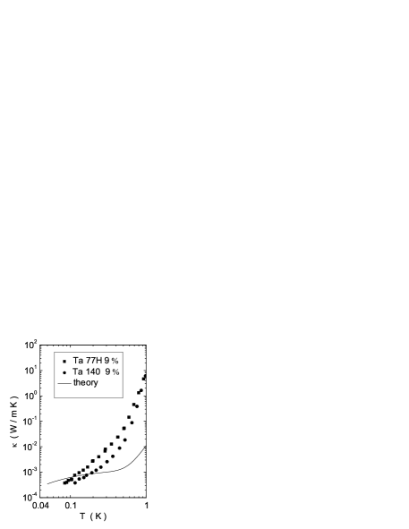
Figure 3: Thermal conductivity for different Ta samples. Experimental data denoted by squares and circles are from Ref. 2. The solid line represents the theoretical curve for $\Lambda_{Ta}=2\times 10^{14}$ m^-2 using the parameter set from Table I. The resonance frequency for Ta is $\Omega_{1}^{+}=2\times 10^{11}$ Hz.

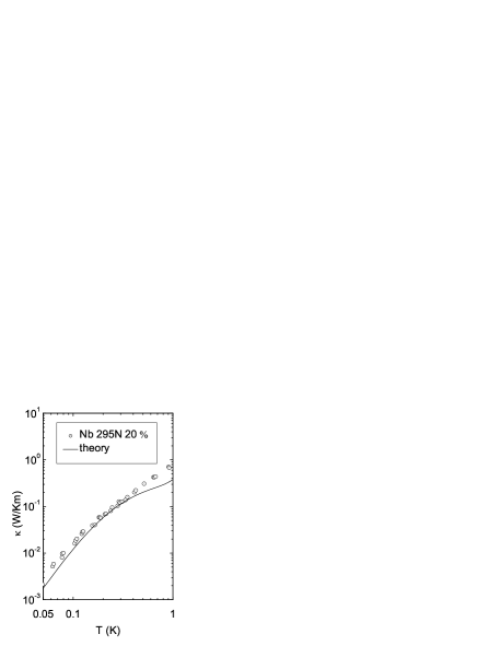
Figure 4: Thermal conductivity for Nb. Experimental data denoted by circles are from Ref. 4. Solid line represents the best fit with $\Lambda_{Nb}=10^{13}$ m^-2 using the parameter set from Table I. The resonance frequency for Nb is $\Omega_{1}^{+}=5\times 10^{11}$ Hz.

where $\theta$ is the Debye temperature. As is well-known, the boundary scattering gives a constant $\tau^{-1}_{c}$ which is determined by geometry of samples. This contribution can be estimated by using the known Casimir formula. $\tau^{-1}_{d}$ is the function of both the decrement $\Delta_{t}$ and the frequency $\omega$ in accordance with Eq.(25). The results of numerical calculations for all the materials are shown in Figs.2-4. The dislocation length is chosen to be $10^{-6}$ m in agreement with the acoustic experiments while the dipole separation $l$ varies from one material to another to get the necessary resonance frequency. The best fits were found for the densities $\Lambda_{Al}=6\times 10^{12}$ m^-2 and $\Lambda_{Nb}=10^{13}$ m^-2. The calculated curve for Ta is shown in Fig.4 with $\Lambda_{Ta}=2\times 10^{14}$ m^-2. Notice that these densities of dipoles differ from those used in the description of the internal friction experiments because the thermal conductivity and internal friction were actually measured on different samples.Pohl:1999 ; Sahl:2001 ; Sahl2:2001 ; Sahl3:2002 ; Was:2002 Therefore, to clarify the problem it would be desirable to measure both the internal friction and the thermal conductivity on the same samples under the same conditions (to avoid stress relaxation and preserve the initial characteristics of dislocation ensembles). It is important to note that the influence of dichotomic noise on the thermal conductivity is found to be negligible. The reason is that the main contribution to the thermal conductivity comes from the region near the resonance frequency of optically vibrating dislocation dipoles. In this case, the term due to the colored noise can be disregarded in the scattering rate ( in Eq.(25) $\Delta_{r}$ becomes much smaller than $\Delta_{p}$, see Fig.1). Thus, in contrast to the internal friction, the dichotomic noise does not influence the thermal conductivity. As is seen from Figs.2-4, there is a good agreement with the experimental data at low temperatures. Notice that a rapid increase of experimental curves with temperature begins in the region where the electronic contribution becomes essential due to an increase of a number of normal electrons in superconducting samples.

V Summary

In this paper, we have shown that the presence of a stationary random process in dislocation ensemble caused by the external perturbation markedly modifies the decrement in the low-frequency range. First, the decrement does not depend on either frequency or temperature at low temperatures and, second, its value becomes much higher in comparison with the Granato-Lücke classical case of periodically affected dislocations. Both these findings agree well with the experimental data. At the same time, an explicit type and probabilistic characteristics of the proposed stochastic process are still not understood because dislocation ensembles show a very complicated dynamics. In fact, by introducing the dichotomic noise we simplify the problem of the nonlinear dynamics of dislocation dipoles to the linear one. We have considered the influence of both external force and colored noise on the internal friction. We have also calculated the contribution to the thermal conductivity due to dislocation dipoles. The concept of dislocation dipoles allows us to obtain the required resonance frequency and, as a consequence, to describe the experimental results for all three plastically deformed metals. It was found that the dichotomic noise does not play any essential role in the thermal conductivity.

Nevertheless, it is still impossible to say that the colored noise in the dislocation ensemble is the only way to explain the experimentally observed damping in Refs. Pohl:1999, ; Sahl3:2002, , and Was:2002, . The purpose of our paper was to draw attention to the fact that this mechanism gives an important contribution to the damping at low temperatures. A good agreement with the experiment was obtained by appropriate choice of two arbitrary parameters noticed above. There are other known mechanisms of damping which could be of importance to explain the experimental data.

One of them was suggested in Ref. Pohl:1999, where the tunneling of some entities (presumably dislocations or dislocation kinks) was discussed as a possible reason for a large internal friction observed in plastically deformed metals at low temperatures. Theoretically, the structures, energy barriers, effective masses, and quantum tunneling rates for dislocation kinks and jogs in copper screw dislocations were determined in Ref. Vegge:2001, by using the molecular-dynamics calculations. It was found that for dislocation kinks in screw dislocations both the energy barrier and the effective mass are markedly reduced so that tunneling should occur readily. The kink tunneling is very sensitive to both the effective mass and the Peierls-like barrier for migration along the dislocation which, in turn, depend on the spatial extent of the kink. In particular, for wide kinks the barrier grows exponentially with decreasing kink width Vegge:2001 . Hence, even a minor change of the kink width results in the substantial variation of the WKB factor (suppressing quantum tunneling). Notice that the value of the kink width used in Refs. Sahl:2001, ; Sahl2:2001, ; Sahl3:2002, for Al, Ta and Nb ($w=5b\sim 1.4$ nm) is about three times shorter than that in Ref. Vegge:2001, for Cu. Besides, typically kink tunneling is suppressed by dissipation (see, e.g., Ref. Hikata:1985, ). In addition, unfortunately both the resonance frequency and the scattering cross-section of the tunneling process are not yet available. This gives no way of calculating the contribution to the thermal conductivity within the kink tunneling model. Therefore, additional investigations within the tunneling kink model are necessary to describe a series of experiments in plastically deformed Al, Ta and Nb.Pohl:1999 ; Sahl:2001 ; Sahl2:2001 ; Sahl3:2002 ; Was:2002

As another possible mechanism, the concept of kinks moving in the secondary Peierls potential was suggested for the description of observed experimental data.Sahl:2001 ; Sahl2:2001 ; Sahl3:2002 Despite a good agreement between the results of the kink model and the experiment, two comments are in order. First, it was found that a good fit for the thermal conductivity takes place only for a surprisingly large number of kinks ($\sim 500$) per dislocation line of length $~{}10^{-6}$m. In this case, the separation between kinks turns out to be 2nm. This value is comparable with the kink width $w\sim 1.4$ nm used in Refs. Sahl:2001, ; Sahl2:2001, ; Sahl3:2002, . At the same time, the radiation mechanism proposed in Ref. Hikata:1974, is essentially based on the long-range interaction between kinks and is only valid when the separation between kinks is large compared to the kink width (otherwise the interaction between kinks may change drastically) Seeger:1966 . Second, within the kink model the internal friction significantly (as a third power) depends on the Peierls stress whose reliable estimation is a complex experimental task Friedel:1964 . As a final remark, at large densities the interaction between dislocations is of importance, hence the complex dislocation dynamics is to be expected.

Table 1: Materials constant for Al (from Ref. 3), Ta (from Ref. 2), and Nb (from Ref. 4).

Table 2: Low frequency internal friction calculated according to Eq.(29) for different metals.