Microscopic modelling of doped manganites

Abstract

Colossal magneto-resistance manganites are characterised by a complex interplay of charge, spin, orbital and lattice degrees of freedom. Formulating microscopic models for these compounds aims at meeting to conflicting objectives: sufficient simplification without excessive restrictions on the phase space. We give a detailed introduction to the electronic structure of manganites and derive a microscopic model for their low energy physics. Focussing on short range electron-lattice and spin-orbital correlations we supplement the modelling with numerical simulations.

1 Introduction

Mixed-valence manganese oxides of perovskite structure have been studied for more than fifty years [1, 2]. However, many of their peculiar properties are still rather poorly understood. About a decade ago the observation of the so-called colossal magneto-resistance effect (CMR) [3, 4, 5] moved these materials again into the focus of intense research activity [6, 7, 8]. It turned out soon that the complex electronic and magnetic properties of the manganites as well as their rich phase diagram depend on a close interplay of almost all degrees of freedom known in solid state physics, namely itinerant charges, localised spins, electronic orbitals, and lattice vibrations. To separate important and less important degrees of freedom and to work out the essential low energy physics are therefore two particularly crucial factors for any microscopic description of these interesting compounds. In the present article we give a detailed introduction to the electronic structure of manganites and derive a microscopic model, which includes the dynamics of charge, spin, orbital and lattice degrees of freedom on a quantum mechanical level. We also discuss potential further simplifications and complement the work with a review of previous numerical studies of the derived model.

2 Crystal structure and symmetries

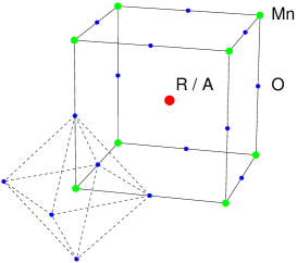
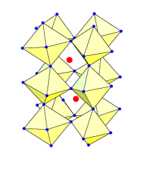
Figure 1: Left: Idealised perovskite structure (space group $Pm3m$). Right: Real structure of LaMnO₃ at $T=1.5\,K$ (orthorhombic, space group $Pnma$) [9].

The structural phase diagrams observed for CMR manganites are almost as rich as their electronic and magnetic counterparts (for a review see, e.g., Ref. [6]). Consider, for example, the undoped parent compound LaMnO₃. At low temperature its structure is characterised by the orthorhombic space group $Pnma$ [9], but doping with strontium, La_1-xSr_xMnO₃, will transform the system to the triclinic space group $R\bar{3}c$ at $x\approx 0.175$ [10, 9]. On the other hand, similar structural transitions occur with increasing temperature [11]. However, nearly all of these crystal arrangements can be understood in terms of distortions of the ideal perovskite structure shown in Figure 1. Here each manganese ion is surrounded by an octahedron of oxygen atoms, whereas the large rare earth (R) or alkaline earth atoms (A), used as dopants, occupy the centre of the cube formed by the manganese sites.

Table 1: The four symmetry operations that generate the cubic point group $O_{h}$, the corresponding notation as well as the action on the position vector.

• Operation	Symbol	Coordinate transformation
  inversion	$I$	$(x,y,z)$	$\rightarrow$	$(-x,-y,-z)$
  4-fold rotation about $x$-axis	$C_{4}^{x}$	$(x,y,z)$	$\rightarrow$	$(x,-z,y)$
  4-fold rotation about $z$-axis	$C_{4}^{z}$	$(x,y,z)$	$\rightarrow$	$(-y,x,z)$
  3-fold rotation about diagonal	$C_{3}^{d}$	$(x,y,z)$	$\rightarrow$	$(z,x,y)$

For a theoretical description it is thus quite natural to start from the above ideal cubic structure, and to account for deviations by including (dynamical) lattice distortions, i.e., phonons, into the microscopic model. Since the cubic site symmetry of the manganese is particularly important, and since its properties and the corresponding notation are frequently used throughout the article, let us first recall some of the basic features of the cubic point symmetry group $O_{h}$. The group $O_{h}$ consists of 48 symmetry operations which can all be generated by the inversion of space and the 3 basic rotations listed in Table 1. Since the rotations commute with the inversion the group $O_{h}$ can be represented as a direct product, $O_{h}=O\otimes C_{i}$, of the inversion group $C_{i}$ and the group $O$, which is formed by the rotations only. With respect to inversion every function can be decomposed into an even ($g$) and an odd ($u$) part, which reflects the two irreducible representations of $C_{i}$ with characters $1$ and $-1$, respectively. Similarly, every irreducible representation of $O$ leads to an even and an odd irreducible representation of $O_{h}$. Given the five irreducible representations of $O$ listed in Table 2 we thus find ten irreducible representations of the full cubic point group $O_{h}$, denoted by $A_{1g}$, $A_{1u}$, $A_{2g}$, etc. Here we follow the notation commonly used in the literature (see, e.g., the textbook of Griffith [12]).

Table 2: The five irreducible representations of the cubic group $O$, the notation used for standard basis elements, examples of corresponding functions, and transformation properties with respect to the group generators. Note that we rotate the functions, not the coordinate system.

• irred.		basis		transformation properties
  repr.	dim.	element	example	$C_{4}^{z}$	$C_{4}^{x}$	$C_{3}^{d}$
  $A_{1}$	1	$a_{1}$	$1$	$a_{1}$	$a_{1}$	$a_{1}$
  $A_{2}$	1	$a_{2}$	$xyz$	$-a_{2}$	$-a_{2}$	$a_{2}$
  $E$	2	$\theta$	$3z^{2}-r^{2}$	$\theta$	$-\frac{1}{2}\theta-\frac{\sqrt{3}}{2}\varepsilon$	$-\frac{1}{2}\theta+\frac{\sqrt{3}}{2}\varepsilon$
  		$\varepsilon$	$x^{2}-y^{2}$	$-\varepsilon$	$-\frac{\sqrt{3}}{2}\theta+\frac{1}{2}\varepsilon$	$-\frac{\sqrt{3}}{2}\theta-\frac{1}{2}\varepsilon$
  $T_{1}$	3	$x$	$x$	$y$	$x$	$y$
  		$y$	$y$	$-x$	$z$	$z$
  		$z$	$z$	$z$	$-y$	$x$
  $T_{2}$	3	$\xi$	$yz$	$-\eta$	$-\xi$	$\eta$
  		$\eta$	$zx$	$\xi$	$-\zeta$	$\zeta$
  		$\zeta$	$xy$	$-\zeta$	$\eta$	$\xi$

As we know, for example from the coupling of angular momenta, the product of elements belonging to two irreducible representations in general leads to a function that belongs to a reducible representation, which can again be decomposed into irreducible representations. For spins the corresponding coupling coefficients are known as the Clebsch Gordan coefficients, and, of course, for the cubic group analogous coefficients were calculated and are listed, e.g., in Ref. [12]. For illustration consider the product $E\otimes T_{1}$, which leads to a six-dimensional reducible representation that can be decomposed into $T_{1}$ and $T_{2}$. In terms of the above basis functions we find

$$x^{\prime}=-\frac{1}{2}\theta\otimes x+\frac{\sqrt{3}}{2}\varepsilon\otimes x\,,\qquad\qquad \xi^{\prime}=-\frac{\sqrt{3}}{2}\theta\otimes x-\frac{1}{2}\varepsilon\otimes x{}\,,$$

$$y^{\prime}=-\frac{1}{2}\theta\otimes y-\frac{\sqrt{3}}{2}\varepsilon\otimes y\,,\qquad\qquad \eta^{\prime}=\frac{\sqrt{3}}{2}\theta\otimes y-\frac{1}{2}\varepsilon\otimes y\,,$$ (1)

$$z^{\prime}=\theta\otimes z\,,\qquad\qquad \zeta^{\prime}=\varepsilon\otimes z\,,{}$$

and obviously the new (dashed) functions fulfil the transformation properties of basis functions of $T_{1}$ and $T_{2}$.

3 Coulomb interaction and local electronic structure

Considering the end members of the manganite series R_1-xA_xMnO₃ at doping $x=0$ and $1$, respectively, within a simplified ionic description the different constituents are assigned the formal valences R³⁺ Mn³⁺ O${}_{3}^{2-}$ and A²⁺ Mn⁴⁺ O${}_{3}^{2-}$. This corresponds to always completely filled oxygen $p$-bands and, with increasing $x$, to hole doping of the manganese $d$-shell, $d^{4}\rightarrow d^{3}$. To some degree already the early doping dependent measurements of the local magnetic moment in La_1-xCa_xMnO₃ by Wollan and Koehler [2] confirm this general picture, but also recent band structure calculations [13, 14] and spectroscopic experiments [15, 16, 17] are indicative of manganese $3d$ conduction bands. Although these bands are partially subject to hybridisation with neighbouring oxygen $2p$ states, it is thus reasonable and common to consider Mn $d$ electrons as the starting point of a microscopic modelling, and proceed along the line which is called the weak-field coupling scheme [12].

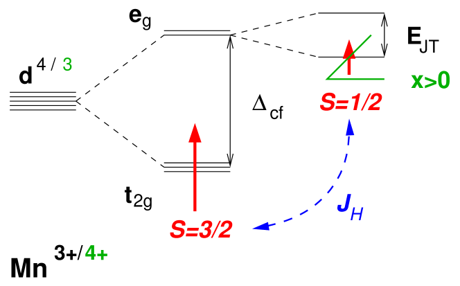
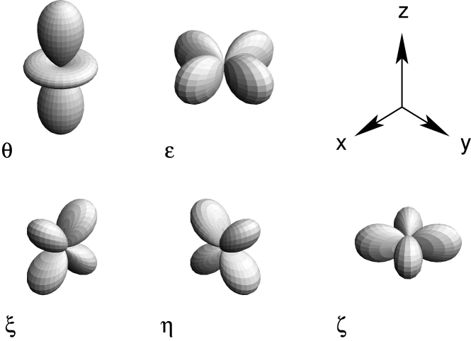
Figure 2: Left: The local electronic structure of Mn $3d$ electrons in a cubic crystal field. Right: Angular structure of the $e_{g}$ and $t_{2g}$ single electron wave functions.

The spherical harmonics $Y_{l,m}$ with $l=2$, which describe the angular part of the $d$ shell, are all even with respect to inversions. Comparing with Table 2 we thus find that these functions can be combined to yield basis functions of the irreducible representations $E_{g}$ and $T_{2g}$ of $O_{h}$,

$$\theta=Y_{2,0}=\sqrt{\frac{5}{16\pi}}\frac{3z^{2}-r^{2}}{r^{2}}\,,\qquad \xi=i\,\frac{Y_{2,+1}+Y_{2,-1}}{\sqrt{2}}=\sqrt{\frac{15}{4\pi}}\frac{yz}{r^{2}}\,,{}$$

$$\varepsilon=\frac{Y_{2,+2}+Y_{2,-2}}{\sqrt{2}}=\sqrt{\frac{5}{16\pi}}\frac{x^{2}-y^{2}}{r^{2}}\,,\qquad \eta=-\,\frac{Y_{2,+1}-Y_{2,-1}}{\sqrt{2}}=\sqrt{\frac{15}{4\pi}}\frac{zx}{r^{2}}\,,$$

$$\zeta=-i\,\frac{Y_{2,+2}-Y_{2,-2}}{\sqrt{2}}=\sqrt{\frac{15}{4\pi}}\frac{xy}{r^{2}}\,.{}$$

Consequently, within the cubic crystal field the five degenerate $d$ levels split into an $E_{g}$ orbital doublet and a $T_{2g}$ orbital triplet. Taking into account the spatial structure of the above wavefunctions and the overlap with neighbouring oxygen electrons, we find that the $t_{2g}$ orbitals are lower in energy compared to $e_{g}$. The magnitude of this crystal field splitting, $\Delta_{\rm cf}$, varies with the occupancy of the levels, typical values for the manganites are of the order of 1.5 to 2.5 eV [15].

So far we considered only the single-electron picture, but for the manganites the on-site Coulomb interaction is strong and thus of particular importance. Before describing the many-electron states of manganese ions in detail, let us review some of the basic facts for the Coulomb interaction of $d$ electrons. Expanding the Coulomb interaction between two charges in terms of spherical harmonics,

$$\quad V=\frac{e^{2}}{|\vec{r}_{1}-\vec{r}_{2}|}=\frac{e^{2}}{r_{>}}\sum_{k=0}^{\infty}\left(\frac{r_{<}}{r_{>}}\right)^{k}\frac{4\pi}{2k+1}\sum_{p=-k}^{k}Y_{kp}(\theta_{1},\phi_{1})Y_{kp}^{*}(\theta_{2},\phi_{2})$$ (3)

with $r_{>}=\max(r_{1},r_{2})$ and $r_{<}=\min(r_{1},r_{2})$, we find that the matrix element between different single electron functions $\psi_{\alpha}=R_{n_{\alpha}l_{\alpha}}Y_{l_{\alpha}m_{\alpha}}s_{\sigma_{\alpha}}$ is given by

$$\langle\psi_{\alpha}\psi_{\beta}|V|\psi_{\gamma}\psi_{\delta}\rangle = \sum_{k=0}^{\infty}F^{k}_{\alpha\beta\gamma\delta}\,c^{k}_{l_{\alpha}m_{\alpha};l_{\gamma}m_{\gamma}}\,c^{k}_{l_{\beta}m_{\beta};l_{\delta}m_{\delta}}\,\delta_{m_{\alpha}+m_{\beta},m_{\gamma}+m_{\delta}}\,\delta_{\sigma_{\alpha},\sigma_{\gamma}}\delta_{\sigma_{\beta},\sigma_{\delta}}\,,{}$$

$$F^{k}_{\alpha\beta\gamma\delta} = \langle R_{n_{\alpha}l_{\alpha}}R_{n_{\beta}l_{\beta}}|\frac{e^{2}r_{<}^{k}}{r_{>}^{k+1}}|R_{n_{\gamma}l_{\gamma}}R_{n_{\delta}l_{\delta}}\rangle\,,$$ (4)

$$c^{k}_{lm;l^{\prime}m^{\prime}} = \sqrt{\frac{4\pi}{2k+1}}\ \langle Y_{lm}|Y_{km-m^{\prime}}Y_{l^{\prime}m^{\prime}}\rangle\,.{}$$

Here we already made use of the fact that the Coulomb interaction preserves the $z$ component of the angular momentum. However, the special structure of the matrix elements $c^{k}_{lm;l^{\prime}m^{\prime}}$ imposes further restrictions on the expansion index $k$ and suggests a close relation to Clebsch Gordan coefficients. Indeed, long ago Racah [18] derived

$$c^{k}_{lm;l^{\prime}m^{\prime}} = (-1)^{g-l}\sqrt{\frac{1}{2}(2l^{\prime}+1)C_{lkl^{\prime}}}\ {\left(\begin{array}[]{cc|c}{l^{\prime}}&{k}&{l}\\ {m^{\prime}}&{m-m^{\prime}}&{m}\end{array}\right)}\,,$$ (7)

$$C_{lkl^{\prime}} = \cases{0&for $l+l^{\prime}+k$ odd\,,\\ \frac{2(l+l^{\prime}-k)!(l+k-l^{\prime})!(l^{\prime}+k-l)!g!^{2}}{(l+l^{\prime}+k+1)!(g-l)!^{2}(g-l^{\prime})!^{2}(g-k)!^{2}}&for $2g:=l+l^{\prime}+k$ even\,,}{}$$

which leads to the conditions of even $l+l^{\prime}+k$ and $|l-l^{\prime}|\leq k\leq l+l^{\prime}$. For the present case of $3d$ electrons the values of $k$ are thus restricted to $k=0,2,4$, and the Coulomb matrix elements reduce to a sum of only three terms,

$$\langle\psi_{\alpha}^{3d}\psi_{\beta}^{3d}|V|\psi_{\gamma}^{3d}\psi_{\delta}^{3d}\rangle=\sum_{\kappa=0}^{2}F^{2\kappa}\,c^{2\kappa}_{2,m_{\alpha};2,m_{\gamma}}\,c^{2\kappa}_{2,m_{\delta};2,m_{\beta}}\,\delta_{m_{\alpha}+m_{\beta},m_{\gamma}+m_{\delta}}\,\delta_{\sigma_{\alpha},\sigma_{\gamma}}\delta_{\sigma_{\beta},\sigma_{\delta}}\,.$$ (8)

In realistic situations the integrals over the radial parts of the wave functions,

$$F^{k}=\langle R_{32}(r_{1})R_{32}(r_{2})|\frac{e^{2}r_{<}^{k}}{r_{>}^{k+1}}|R_{32}(r_{1})R_{32}(r_{2})\rangle\,,$$ (9)

are usually hard to calculate exactly and are therefore taken as free parameters which depend on details of the considered ions and compounds. Instead of the above $F^{k}$ the so-called Racah parameters,

$$A=F^{0}-F^{4}/9,\quad B=\frac{9F^{2}-5F^{4}}{441},\quad C=\frac{5F^{4}}{63}\,,$$ (10)

are more common, because they simplify the notation of the Coulomb matrix elements. Since the $F^{k}$ are positive and monotonously decreasing in $k$ [19, 12], the Racah parameters are positive as well. In addition, for many transition metals the ratio $C/B$ is almost constant and of the order of $4$ to $5$. Later we make use of this by expressing the Coulomb interaction in terms of just two parameters $U$ and $J_{h}$. In Table 3 we show estimates of $A$, $B$ and $C$ for manganese obtained from spectroscopic data.

Table 3: Different estimates for the Racah parameters of manganese ions (in eV) and corresponding references.

• ion	$A$	$B$	$C$	reference
  Mn2+	6.05	0.107	0.477	[20, 21]
  	5.43	0.1190	0.4122	[22]
  Mn3+	6.40	0.120	0.552	[20, 21]
  	5.26	0.120	0.552	[23, 21]
  Mn4+	6.58	0.132	0.610	[20, 21]

Based on the above introduction we are now in the position to construct many-electron eigenstates of the Coulomb interaction for a single ion in a cubic crystal field, which define the starting point of our modelling. Neglecting spin-orbit coupling, which is usually very small for compounds of the first transition metal series, the Coulomb matrix can be decomposed into blocks of given spin and cubic symmetry. Especially for the low-energy states it turns out that this symmetrisation diagonalises the Coulomb matrix, i.e. we immediately find the ground-states of the $n$ electron systems. Taking into account the crystal field splitting, for the Mn⁴⁺ ion ($d^{3}$) the ground state is obtained by triply occupying the $t_{2g}$ levels and forming a state of maximum spin (Hunds rule). This leads to the spin quartet and orbital singlet ${}^{4}\!A_{2}$, which in terms of the fermionic creation operators $c^{\dagger}_{\nu\sigma}$ reads

$$|a_{2},\frac{3}{2},m\rangle=\sqrt{\frac{(\frac{3}{2}-m)!}{3!(\frac{3}{2}+m)!}}\,(S^{+})^{(\frac{3}{2}+m)}\,c^{\dagger}_{\xi\downarrow}c^{\dagger}_{\eta\downarrow}c^{\dagger}_{\zeta\downarrow}|0\rangle\,,$$ (11)

and its Coulomb energy is $\epsilon(^{4}\!A_{2})=3A-15B$. For Mn³⁺ ($d^{4}$) the ground state is a spin quintet and orbital doublet ${}^{5}E$ with components

$$|\theta,2,m\rangle = +\,\sqrt{\frac{(2-m)!}{4!(2+m)!}}\,(S^{+})^{(2+m)}\,c^{\dagger}_{\varepsilon\downarrow}c^{\dagger}_{\xi\downarrow}c^{\dagger}_{\eta\downarrow}c^{\dagger}_{\zeta\downarrow}|0\rangle\,,$$ (12)

$$|\varepsilon,2,m\rangle = -\,\sqrt{\frac{(2-m)!}{4!(2+m)!}}\,(S^{+})^{(2+m)}\,c^{\dagger}_{\theta\downarrow}c^{\dagger}_{\xi\downarrow}c^{\dagger}_{\eta\downarrow}c^{\dagger}_{\zeta\downarrow}|0\rangle\,,$$ (13)

which reflects the freedom of choosing one of the $e_{g}$ levels when adding another electron to the $d^{3}$ system and requiring strong Hunds rule coupling, i.e. maximal spin. The Coulomb energy of the ${}^{5}E$ state is $\epsilon(^{5}E)=6A-21B$. Note also that in the $\theta$ component of the many-electron state the $\varepsilon$ single-electron level is occupied, and vice versa, which is caused by the $d^{3}$ state belonging to $A_{2}$.

4 Perturbation theory in the electronic hopping

The energy difference between the above ionic ground states and the corresponding lowest excitations is given by the crystal field splitting $\Delta_{\rm cf}$, or by a Coulomb energy of at least $8B+3C$. Both energy scales are large compared to the hopping matrix element of $e_{g}$ electrons between two neighbouring manganese sites, which is of the order of $t\approx 0.3$ to $0.4$ eV [24, 25, 26]. The hopping of $t_{2g}$ electrons, $t_{\pi}$, is even smaller. The derivation of an effective low-energy Hamiltonian can thus be based on a perturbative expansion in terms of $t_{(\pi)}$. Since the transfer of electrons between different manganese sites always proceeds via the completely filled $2p$ shell of bridging oxygen sites, the hopping matrix elements acquire a particular orbital dependence, which leads to effective spin-orbital interactions and finally causes all the interesting patterns of orbital ordering or disorder observed in the manganites. As Figure 3 illustrates for bonds in $z$-direction, the $\varepsilon$ orbital by symmetry has no overlap between any of the three oxygen $p$ orbitals, whereas for the $\theta$ orbital only the overlap to $p_{z}$ is finite. Similarly we find that the $t_{2g}$ orbitals have finite overlap at most to one of $p_{x}$ or $p_{y}$, and we can thus summarise all possible hopping processes in $z$-direction with the Hamiltonian

$$\quad H_{\rm hopp}^{z}=-\sum_{i,\sigma}\left[t\,c^{\dagger}_{i,\theta\sigma}c_{i+z,\theta\sigma}+t_{\pi}(c^{\dagger}_{i,\xi\sigma}c_{i+z,\xi\sigma}+c^{\dagger}_{i,\eta\sigma}c_{i+z,\eta\sigma})+{\rm H.c.}\right]$$ (14)

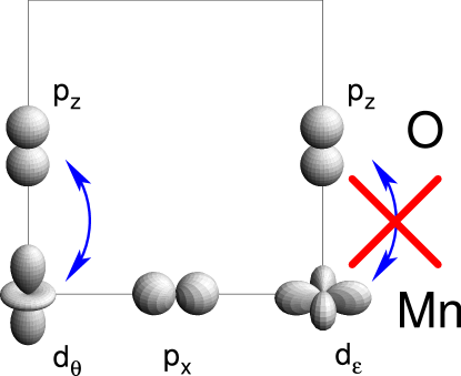
Figure 3: Illustration of the orbital anisotropy of the electronic hopping via bridging oxygen sites.

At first glance the situation for $x$ and $y$-bonds appears to be more involved. However, using the cubic point symmetry operations, e.g. the diagonal rotation $C_{3}^{d}$, we can easily derive the corresponding hopping matrix elements by simply inserting the rotated orbitals into Equation (14). More formally we introduce the operators

$$R_{x} =(C_{3}^{d})^{1}\,,\ R_{y}=(C_{3}^{d})^{2}=(C_{3}^{d})^{-1}\,,\ R_{z}=(C_{3}^{d})^{3}=1\,,$$ (15)

$$C_{3}^{d} :\ c_{\theta/\varepsilon}\rightarrow-(c_{\theta/\varepsilon}\mp\sqrt{3}c_{\varepsilon/\theta})/2\,;\ c_{\xi/\eta/\zeta}\rightarrow c_{\eta/\zeta/\xi}\,,{}$$

and obtain for the complete hopping Hamiltonian

$$\quad H_{\rm hopp}=-\sum_{i,\delta,\sigma}R_{\delta}\left[t\,c^{\dagger}_{i,\theta\sigma}c_{i+\delta,\theta\sigma}+t_{\pi}(c^{\dagger}_{i,\xi\sigma}c_{i+\delta,\xi\sigma}+c^{\dagger}_{i,\eta\sigma}c_{i+\delta,\eta\sigma})+{\rm H.c.}\right]$$ (16)

In general $H_{\rm hopp}$ connects the ionic ground state at one site to a large number of Coulomb excited states at the other site. A complete description of the electronic subsystem would thus require a huge local Hilbert space, which includes basically all ionic excitations. However, these high-energy excitations are irrelevant for most of the features we want to model, and we thus restrict the local Hilbert space to the ionic ground states derived in Section 3 and account for the excitations in the framework of standard degenerate perturbation theory. Then the first order of the effective Hamiltonian is given by the matrix elements of $H_{\rm hopp}$ between basis states of the form (11) and (12) on neighbouring sites. These basis states differ in the total on-site spin $|\vec{S}_{i}|$. To achieve an uniform description it is thus convenient to rewrite the spin degrees of freedom in terms of Schwinger bosons [27], which provide a simple means for changing $|\vec{S}_{i}|$,

$$S_{i}^{+}=a_{i,\uparrow}^{\dagger}a_{i,\downarrow}\,,\qquad S_{i}^{z}=(a_{i,\uparrow}^{\dagger}a_{i,\uparrow}-a_{i,\downarrow}^{\dagger}a_{i,\downarrow})/2\,,{}$$

$$S_{i}^{-}=a_{i,\downarrow}^{\dagger}a_{i,\uparrow}\,,\qquad |\vec{S}_{i}|=(a_{i,\uparrow}^{\dagger}a_{i,\uparrow}+a_{i,\downarrow}^{\dagger}a_{i,\downarrow})/2\,.$$ (17)

In addition, we can also reduce the number of fermionic operators and introduce hole operators $d_{i,\theta}^{(\dagger)}$ and $d_{i,\varepsilon}^{(\dagger)}$ instead. The orbital part of our basis states and corresponding projection operators then read

$$|\theta\rangle=d^{\dagger}_{\theta}|0\rangle\,,\qquad |\varepsilon\rangle=d^{\dagger}_{\varepsilon}|0\rangle\,,\qquad |a_{2}\rangle=d^{\dagger}_{\theta}d^{\dagger}_{\varepsilon}|0\rangle\,,{}$$

$$P^{\theta}=n_{\theta}(1-n_{\varepsilon})\,,\qquad P^{\varepsilon}=n_{\varepsilon}(1-n_{\theta})\,,\qquad P^{a_{2}}=n_{\varepsilon}n_{\theta}\,,$$ (18)

where the vacuum $|0\rangle$ is invariant under cubic symmetry operations, i.e. belongs to $A_{1}$. Calculating the effective hopping matrix element for a $z$-bond we are mainly concerned with the spin part, whereas the orbital part is rather trivial, since only $\theta$ electrons are allowed to tunnel. Given the spin-$2$ state $|\varepsilon,2,m\rangle$ on site $i$ and the spin-$3/2$ state $|a_{2},3/2,m^{\prime}\rangle$ on site $j$ the hopping of a $\theta$ electron will transfer a spin-$1/2$ from $i$ to $j$. Projecting the new states onto our basis will lead to $|a_{2}\rangle$ at $i$ and $|\varepsilon\rangle$ at $j$. In addition, the hopping conserves the total bond spin $\vec{S}_{i}+\vec{S}_{j}$. Combining all three properties of the process, i.e. transfer of a spin-$1/2$, increase of $|\vec{S}_{j}|$ and lowering of $|\vec{S}_{i}|$, as well as conservation of $\vec{S}_{i}+\vec{S}_{j}$, in terms of Schwinger bosons we can almost guess the effective matrix element to be proportional to $a_{j,\uparrow}^{\dagger}a_{i,\uparrow}+a_{j,\downarrow}^{\dagger}a_{i,\downarrow}$. Indeed, a more careful calculation [28] of the double-exchange [29, 30] matrix element shows that corresponding prefactor is $-t/(2S+1)$, where $S$ is the amplitude of the shorter of the two on-site spins. For a bond in $z$-direction the first order of the effective Hamiltonian is thus given by

$$H^{1,z}_{i,j}=-\frac{t}{4}\left(a_{i,\uparrow}a^{\dagger}_{j,\uparrow}+a_{i,\downarrow}a^{\dagger}_{j,\downarrow}\right)\ d^{\dagger}_{i,\theta}n_{i,\varepsilon}d_{j,\theta}n_{j,\varepsilon}+{\rm H.c.}$$ (19)

Note that the amplitude of the local spin is restricted by $2|\vec{S}_{i}|=a^{\dagger}_{i,\uparrow}a_{i,\uparrow}+a^{\dagger}_{i,\uparrow}a_{i,\uparrow}=5-(n_{i,\varepsilon}+n_{i,\theta})$.

Table 4: Excitations of a single manganese ion that can be reached by adding or subtracting an $e_{g}$ or $t_{2g}$ electron to the basis states ${}^{5}E$ and ${}^{4}\!A_{2}$. Starred Coulomb energies in the last column are approximate (see text and Ref. [12]).

• initial state	operation		final state	energy
  ${}^{5}E[t_{2}^{3}(^{4}\!A_{2})e]$	$d^{4}\nearrow d^{5}$	$c_{e\downarrow}^{\dagger}$	${}^{6}\!A_{1}[t_{2}^{3}(^{4}\!A_{2})e^{2}(^{3}\!A_{2})]$	$10A-35B$
  		$c_{e\uparrow}^{\dagger}$	${}^{4}\!A_{1}[t_{2}^{3}(^{4}\!A_{2})e^{2}(^{3}\!A_{2})]$	$10A-25B+5C$
  			${}^{4}\!A_{2}[t_{2}^{3}(^{4}\!A_{2})e^{2}(^{1}\!A_{1})]$	$10A-13B+7C$
  			${}^{4}E[t_{2}^{3}(^{4}\!A_{2})e^{2}(^{1}E)]$	$10A-21B+5C^{*}$
  		$c_{t_{2}\uparrow}^{\dagger}$	${}^{4}T_{1}[t_{2}^{4}(^{3}T_{1})e]$	$10A-25B+6C^{*}$
  			${}^{4}T_{2}[t_{2}^{4}(^{3}T_{1})e]$	$10A-17B+6C^{*}$
  	$d^{4}\searrow d^{3}$	$c_{e\downarrow}$	${}^{4}\!A_{2}[t_{2}^{3}]$	$3A-15B$
  		$c_{t_{2}\downarrow}$	${}^{4}T_{1}[t_{2}^{2}(^{3}T_{1})e]$	$3A-3B^{*}$
  			${}^{4}T_{2}[t_{2}^{2}(^{3}T_{1})e]$	$3A-15B$
  ${}^{4}\!A_{2}[t_{2}^{3}]$	$d^{3}\nearrow d^{4}$	$c_{e\downarrow}^{\dagger}$	${}^{5}E[t_{2}^{3}(^{4}\!A_{2})e]$	$6A-21B$
  		$c_{e\uparrow}^{\dagger}$	${}^{3}E[t_{2}^{3}(^{4}\!A_{2})e]$	$6A-13B+4C^{*}$
  		$c_{t_{2}\uparrow}^{\dagger}$	${}^{3}T_{1}[t_{2}^{4}]$	$6A-15B+5C^{*}$
  	$d^{3}\searrow d^{2}$	$c_{t_{2}\downarrow}$	${}^{3}T_{1}[t_{2}^{2}]$	$A-5B^{*}$

Table 5: The matrix elements $\langle d^{n}d^{m}|H_{\rm hopp}^{z}|d^{n-1}d^{m+1}\rangle=O_{\alpha\beta}\,S(x)\,t_{(\pi)}$ together with the corresponding excitation energies $\Delta\epsilon$. For brevity we denote vanishing matrix elements with dots, write $x=\vec{S}_{i}\vec{S}_{j}$ and give the squared $S(x)$.

• $O_{\alpha\beta}$				$S(x)^{2}$	$t_{(\pi)}$	$\Delta\epsilon$
  $\theta\theta$	$\theta\varepsilon$	$\varepsilon\theta$	$\varepsilon\varepsilon$
  $\cdot$	$\cdot$	$-1$	$\cdot$	$\frac{3}{5}\frac{4-x}{16}$	$t$	$A+2B+5C$
  $\cdot$	$\cdot$	$\cdot$	$-1$	$\frac{4-x}{16}$	$t$	$A+14B+7C$
  $\cdot$	$\cdot$	$1$	$\cdot$	$\frac{4-x}{16}$	$t$	$A+6B+5C$
  $\cdot$	$\cdot$	$\cdot$	$-1$	$\frac{4-x}{16}$	$t$	$A+6B+5C$
  $\cdot$	$\cdot$	$-1$	$\cdot$	$\frac{6+x}{10}$	$t$	$A-8B$
  $-\frac{3}{4}$	$\pm\frac{\sqrt{3}}{4}$	$\pm\frac{\sqrt{3}}{4}$	$-\frac{1}{4}$	$\frac{4-x}{8}$	$t_{\pi}$	$A+14B+6C$
  $\frac{1}{4}$	$\pm\frac{\sqrt{3}}{4}$	$\pm\frac{\sqrt{3}}{4}$	$\frac{3}{4}$	$\frac{4-x}{8}$	$t_{\pi}$	$A+10B+6C$
  $\mp\frac{\sqrt{3}}{4}$	$\frac{3}{4}$	$-\frac{1}{4}$	$\pm\frac{\sqrt{3}}{4}$	$\frac{4-x}{8}$	$t_{\pi}$	$A+22B+6C$
  $\pm\frac{\sqrt{3}}{4}$	$\frac{1}{4}$	$-\frac{3}{4}$	$\mp\frac{\sqrt{3}}{4}$	$\frac{4-x}{8}$	$t_{\pi}$	$A+2B+6C$
  $\theta a_{2}$	$\varepsilon a_{2}$	$a_{2}\theta$	$a_{2}\varepsilon$
  $\cdot$	$1$	$\cdot$	$\cdot$	$\frac{3-x}{8}$	$t$	$8B+4C$
  $\pm\frac{\sqrt{3}}{2}$	$-\frac{1}{2}$	$\cdot$	$\cdot$	$\frac{3-x}{6}$	$t_{\pi}$	$18B+5C$
  $\frac{1}{2}$	$\pm\frac{\sqrt{3}}{2}$	$\cdot$	$\cdot$	$\frac{3-x}{6}$	$t_{\pi}$	$6B+5C$
  $\cdot$	$\cdot$	$\pm\frac{\sqrt{3}}{2}$	$-\frac{1}{2}$	$\frac{3-x}{6}$	$t_{\pi}$	$2A+6B+6C$
  $\cdot$	$\cdot$	$-\frac{1}{2}$	$\pm\frac{\sqrt{3}}{2}$	$\frac{3-x}{6}$	$t_{\pi}$	$2A+14B+6C$
  			$a_{2}a_{2}$
  			$1$	$\frac{9-4x}{9}$	$t_{\pi}$	$A+10B+5C$

The second order of perturbation theory in $t_{(\pi)}$ is a bit more involved, since now all virtual excitations of the basis states have to be taken into account. In Table 4 we list all eleven many-particle states that can be constructed by adding or subtracting one $e_{g}$ or $t_{2g}$ electron to the basis states from Equations (11) and (12), thereby respecting cubic and spin symmetry. Since usually there are other configurations belonging to the same representations of orbital and spin symmetry, these states are not necessarily eigenstates of the on-site Coulomb interaction. However, since these other states have no overlap to our basis, taking into account the exact Coulomb eigenstates will only slightly modify the energy denominator of the second order terms, but not the general structure of the matrix elements. It is thus sufficient to consider the expectation value of the Coulomb energy in the above configurations, and the corresponding approximate energies are marked with a star in Table 4. Proceeding further, we can now place all pairs of the three basis states on a single Mn-Mn bond and form states of given total bond spin $\vec{S}_{b}$. Then we need to calculate the overlap to all pairs of excited states that are connected to our bond ground-state by a single electron transfer and share the same bond spin $\vec{S}_{b}$. Clearly, there is a reasonable number of different combinations, and the use of some computer algebra system is recommended. Each of the matrix elements

$$\langle d^{n}d^{m}|H_{\rm hopp}|d^{n-1}d^{m+1}\rangle=O_{\alpha\beta}\,S(\vec{S}_{i}\vec{S}_{j})\,t_{(\pi)}\,,\quad\alpha,\beta\in\{\theta,\varepsilon,a_{2}\}$$ (20)

can be decomposed into an orbital part $O_{\alpha\beta}$, a spin part $S(\vec{S}_{i}\vec{S}_{j})$ and the corresponding transfer amplitude $t_{(\pi)}$. In Table 5 we list these components for all $d^{4}d^{4}\rightleftharpoons d^{3}d^{5}$, $d^{4}d^{3}\rightleftharpoons d^{3}d^{4}$, $d^{3}d^{4}\rightleftharpoons d^{2}d^{5}$ and $d^{3}d^{3}\rightleftharpoons d^{2}d^{4}$ excitations for a bond in $z$-direction, i.e. $j=i+z$. Comparing the orbital parts $O_{\alpha\beta}$ with the rotation properties of the $\theta$ and $\varepsilon$ functions given in Table 2, we observe that the $O_{\alpha\beta}$ can be simplified, if we change the orbital quantisation axis from $z$ to $x$ or $y$. For instance, the four matrix elements $-\{3,\sqrt{3},\sqrt{3},1\}/4$ in line 6 of Table 5, which connect the functions $\{\theta\theta,\theta\varepsilon,\varepsilon\theta,\varepsilon\varepsilon\}$ to the appropriate excitation, reduce to a single matrix element $-1$ originating from the bond state $\varepsilon_{x}\varepsilon_{x}$ with $\varepsilon_{x}=-(\sqrt{3}\,\theta+\varepsilon)/2$. Hereafter we use these properties to express some of the interactions with the help of the rotation operators $R_{\delta}$, $\delta\in\{x,y,z\}$.

Putting together all the above pieces we are now in the position to formulate the second order contributions to our effective electronic Hamiltonian. For simplicity, we neglect all terms which involve hopping processes between three sites, and restrict ourselves to those terms, where an electron hops back and forth on a single Mn-Mn bond,

$$H=-\sum_{{\langle ij\rangle}\atop{\alpha_{i}\alpha_{j}\beta_{i}\beta_{j},\Psi}}\frac{|\alpha_{i}\alpha_{j}\rangle\langle\alpha_{i}\alpha_{j}|\,H_{\rm hopp}\,|\Psi\rangle\langle\Psi|\,H_{\rm hopp}\,|\beta_{i}\beta_{j}\rangle\langle\beta_{i}\beta_{j}|}{\Delta\epsilon(\Psi)}\,.$$ (21)

In addition, we follow Ref. [26] by assuming $C\approx 4B$ and introducing new Coulomb parameters $U$ and $J_{h}$, which refer to a Hubbard like on-site repulsion and a Hunds rule coupling, respectively. The actual choice of the relation between $U$, $J_{h}$ and $A$, $B$, $C=4B$ is a matter of convention. Having in mind the undoped compounds and a bond with $d^{4}(^{5}E)$ basis state on each site, we may ascribe $U$ to the minimal energy required for transferring one of the $e_{g}$ electrons and forming a low spin $d^{5}$ state on one of the sites. On the other hand, the excitation with a high-spin $d^{5}$ state should have energy $U-5J_{h}$, where the factor $5$ reminds of the energy difference originating from an exchange term $J_{h}\vec{S}\vec{s}$ with $|\vec{S}|=2$ and $|\vec{s}|=1/2$. This choice leads to

$$U =\epsilon[d^{5}(^{4}\!A_{1})d^{3}(^{4}\!A_{2})]-\epsilon[d^{4}(^{5}E)d^{4}(^{5}E)]=A+2B+5C\,,{}$$

$$5J_{h} =\epsilon[d^{5}(^{4}\!A_{1})d^{3}(^{4}\!A_{2})]-\epsilon[d^{5}(^{6}\!A_{1})d^{3}(^{4}\!A_{2})]=10B+5C\,,$$ (22)

and after some algebra for a $z$-bond we obtain the following contribution of second order in $t_{(\pi)}$

$$H^{2,z}_{i,j} =t^{2}\,\frac{\vec{S}_{i}\vec{S}_{j}-4}{8}\left[\frac{(4U+J_{h})\,P^{\varepsilon}_{i}P^{\theta}_{j}}{5U(U+\frac{2}{3}J_{h})}+\frac{(U+2J_{h})\,P^{\varepsilon}_{i}P^{\varepsilon}_{j}}{(U+\frac{10}{3}J_{h})(U+\frac{2}{3}J_{h})}\right]{}$$ (23)

$$-t^{2}\,\frac{\vec{S}_{i}\vec{S}_{j}+6}{10(U-5J_{h})}\,P^{\varepsilon}_{i}P^{\theta}_{j}+t_{\pi}^{2}\,\frac{\vec{S}_{i}\vec{S}_{j}-4}{8}\left[\frac{R_{x}(P^{\varepsilon}_{i}P^{\varepsilon}_{j})+R_{y}(P^{\varepsilon}_{i}P^{\varepsilon}_{j})}{U+8J_{h}/3}\right.{}$$

$$\ \qquad\left.+\frac{R_{x}(P^{\theta}_{i}P^{\theta}_{j})+R_{y}(P^{\theta}_{i}P^{\theta}_{j})}{U+2J_{h}}+\frac{(2U+\frac{14}{3}J_{h})(R_{x}(P^{\varepsilon}_{i}P^{\theta}_{j})+R_{y}(P^{\varepsilon}_{i}P^{\theta}_{j}))}{(U+4J_{h})(U+\frac{2}{3}J_{h})}\right]{}$$

$$+t^{2}\,\frac{\vec{S}_{i}\vec{S}_{j}-3}{32J_{h}}\,P^{\varepsilon}_{i}P^{a_{2}}_{j}+t_{\pi}^{2}\,\frac{\vec{S}_{i}\vec{S}_{j}-3}{3}\left[\frac{(U-2J_{h})(R_{x}(P^{\varepsilon}_{i}P^{a_{2}}_{j})+R_{y}(P^{\varepsilon}_{i}P^{a_{2}}_{j}))}{\frac{19}{3}J_{h}(2U-\frac{7}{3}J_{h})}\right.{}$$

$$\ \qquad+\left.\frac{(U+\frac{5}{3}J_{h})(R_{x}(P^{\theta}_{i}P^{a_{2}}_{j})+R_{y}(P^{\theta}_{i}P^{a_{2}}_{j}))}{\frac{13}{3}J_{h}(2U-J_{h})}\right]{}$$

$$+t_{\pi}^{2}\,\frac{\frac{4}{9}\vec{S}_{i}\vec{S}_{j}-1}{U+\frac{4}{3}J_{h}}\,P^{a_{2}}_{i}P^{a_{2}}_{j}+{\rm H.c.}$$

The first three terms reproduce the result of Ref. [26] for the undoped compounds, which are characterised by a competition of one ferromagnetic and a number of anti-ferromagnetic spin exchange terms of order $t_{(\pi)}^{2}/U$. The latter, however, are directly coupled to pairs of orbital projectors favouring different patterns of orbital ordering. Upon doping the ferromagnetic double-exchange interaction, Equation (19), comes into play, but also anti-ferromagnetic terms of order $t_{(\pi)}^{2}/J_{h}$ gain importance. Obviously, the complex phase diagram and the different ordering patterns of the manganites are a direct consequence of effects noticeable already on the level of the microscopic Hamiltonian.

5 Electron-phonon interaction

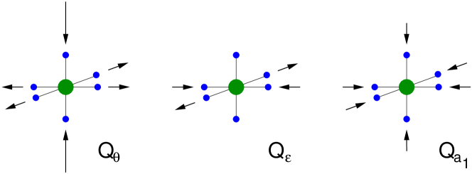
Figure 4: Elongation patterns of the oxygen ions within the $E_{g}$ and $A_{1g}$ vibration modes of a MnO₆ octahedron.

As discussed before, most undoped or weakly doped manganites show long range (Jahn-Teller type) distortions from the ideal perovskite structure, and changes in the magnetic or orbital ordering patterns are usually accompanied by changes in the crystal structure. In addition, modern experimental techniques show that besides these cooperative static effects also dynamic and local properties of the lattice are important for an understanding of the manganites. To name only a few, we may think of x-ray-absorption fine-structure data [31] showing a clear relationship between magnetic order and local lattice distortion, or measurements of the atomic pair-correlation function [32, 33] proving the correlation of electric resistivity and local lattice structure near the metal-insulator transition. It is thus natural to consider electron lattice interactions and, in particular, polaronic effects as an important ingredient of a microscopic description of CMR manganites [34, 35].

Like for the electronic, spin and orbital degrees of freedom, the local environment of the manganese ions is the appropriate starting point also for the modelling of the electron lattice interaction. In Figure 4 we show the basic vibration modes of the MnO₆ octahedron that are even under inversion and thus susceptible for a linear coupling to the $d$ orbitals. The modes $Q_{\theta}$ and $Q_{\varepsilon}$, which belong to the irreducible representation $E_{g}$, are responsible for the Jahn-Teller effect [36, 37], where the system tries to lift the degeneracy of the two ${}^{5}E$ ionic basis states (see Equation (12)) and gain electronic energy by lowering the point symmetry through a distortion of the lattice. As above the electronic degrees of freedom are described by the fermionic operators $d_{\theta/\varepsilon}^{(\dagger)}$, whereas for the phonons we have the bosonic operators $b_{\theta/\varepsilon}^{(\dagger)}$. The interaction between both should be linear in the bosons, bilinear in the fermions, and belong to the irreducible representation $A_{1}$ to form a Hamiltonian that conserves cubic symmetry. These requirements lead to one of the classical Jahn-Teller problems, the so-called $E\otimes e$ model [38, 39]

$$\quad H^{\rm JT}=g\left[(n_{\varepsilon}-n_{\theta})(b^{\dagger}_{\theta}+b_{\theta})+(d^{\dagger}_{\theta}d_{\varepsilon}+d^{\dagger}_{\varepsilon}d_{\theta})(b^{\dagger}_{\varepsilon}+b_{\varepsilon})\right]+\omega\left[b^{\dagger}_{\theta}b_{\theta}+b^{\dagger}_{\varepsilon}b_{\varepsilon}\right]\,,$$ (24)

where the last term refers to the usual harmonic lattice dynamics. For a single ion this model possesses an additional $O(2)$ symmetry, which becomes manifest in the commutation of the Hamiltonian $H^{\rm JT}$ with the $A_{2}$ symmetric operator $(d^{\dagger}_{\theta}d_{\varepsilon}-d^{\dagger}_{\varepsilon}d_{\theta})/2-(b^{\dagger}_{\theta}b_{\varepsilon}-b^{\dagger}_{\varepsilon}b_{\theta})$, and leads to a two-fold degeneracy of every eigenvalue. Whereas for a single ion this seeming contradiction to the common notion of a Jahn-Teller system can be lifted by higher order electron lattice interactions, for realistic compounds like the manganites this symmetry is already broken by the orbitally anisotropic hopping between neighbouring sites, Equation (16). Unfortunately we thereby loose an advantage of this symmetry: the simple tridiagonal structure of the $E\otimes e$ Hamiltonian matrix [38]. Compared to a symmetric hopping, the symmetry-breaking orbital anisotropy may also increases the susceptibility of the system to Jahn-Teller type ordering and polaronic effects, an issue which could be interesting for future studies.

Coming back to the phonon modes of the MnO₆ octahedron, the symmetric mode $Q_{a_{1}}$ should couple to a bilinear fermionic operator belonging to the same $A_{1}$ representation. The most natural operator of this type is the electronic density, and we arrive at the Holstein type [40, 41] Hamiltonian,

$$H^{\rm Hol}=\tilde{g}\,(n_{\theta}+n_{\varepsilon})(b^{\dagger}_{a_{1}}+b_{a_{1}})+\tilde{\omega}\ b^{\dagger}_{a_{1}}b_{a_{1}}\,,$$ (25)

which is well known from polaron physics. Since we use hole operators instead of electrons, we prefer to adjust the expression for the local density such that the ${}^{5}E$ states couple to $Q_{a_{1}}$ but ${}^{4}A_{2}$ does not, $n_{i,\theta}+n_{i,\varepsilon}-2n_{i,\theta}n_{i,\varepsilon}$. Generalising the above types of local electron phonon interaction to the crystal and neglecting the weak dispersion of the optical phonons corresponding to $Q_{\theta}$, $Q_{\varepsilon}$ and $Q_{a_{1}}$, we finally arrive at the Hamiltonian

$$\quad H^{\rm EP} =g\sum_{i}\left[(n_{i,\varepsilon}-n_{i,\theta})(b^{\dagger}_{i,\theta}+b_{i,\theta})+(d^{\dagger}_{i,\theta}d_{i,\varepsilon}+d^{\dagger}_{i,\varepsilon}d_{i,\theta})(b^{\dagger}_{i,\varepsilon}+b_{i,\varepsilon})\right]{}$$

$$+\tilde{g}\sum_{i}(n_{i,\theta}+n_{i,\varepsilon}-2n_{i,\theta}n_{i,\varepsilon})(b^{\dagger}_{i,a_{1}}+b_{i,a_{1}})$$

$$+\omega\sum_{i}\left[b^{\dagger}_{i,\theta}b_{i,\theta}+b^{\dagger}_{i,\varepsilon}b_{i,\varepsilon}\right]+\tilde{\omega}\sum_{i}b^{\dagger}_{i,a_{1}}b_{i,a_{1}}\,.{}$$

6 Discussion of the microscopic model and numerical results

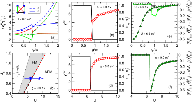
Figure 5: Ground-state properties of the full model, Equation (27), on a four site cluster at doping $x=0$. (a) Evolution of lattice correlations with increasing electron phonon (EP) coupling. (b) Phase diagram of the model without EP coupling; the blue star and arrow mark parameters $U$, $J_{h}$ used in the other panels. (c) Spin and orbital ordering with increasing EP coupling $g$. (d) Spin and orbital ordering with increasing $U$ and $g=0$. (e) Decoupling of spins and orbitals with increasing EP coupling $g$. (f) Spin-orbital correlations at $g=0$. Throughout $J_{h}=0.7$ eV, $t=3t_{\pi}=0.4$ eV, $\omega=\tilde{\omega}=0.07$ eV, $\tilde{g}=g$; see [42] for more details.

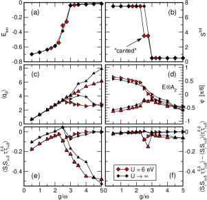
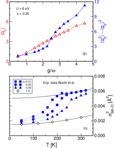
Figure 6: Ground-state properties of the full model, Equation (27), on a four site cluster at doping $x=0.25$. (a) Due to polaron formation the kinetic energy decreases with $g$. (b) At strong $g$ double-exchange is too weak to promote ferromagnetism, i.e. the total spin of the clusters goes to zero. (c) Bond-lengths $\langle q_{x/y}\rangle$ along $x$ and $y$ direction show lattice distortion in the spin disordered phase. (d) The orbital orientation $\varphi$ in the neighbourhood of a hole is orbital-polaron like only for mobile carriers. (e) and (f) Electron-phonon interaction causes an effective decoupling of spin and orbital degrees of freedom. (g) and (h) For increasing $g$ lattice fluctuations show a kink near the FM-AFM transition, quite similar to the experimentally observed behaviour as a function of temperature [31]. See [42, 43] for more details.

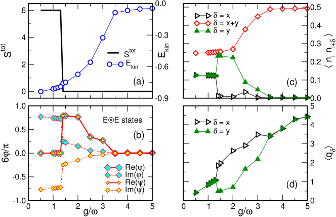
Figure 7: Ground-state properties of the full model, Equation (27), on a four site cluster at doping $x=0.5$. (a) Similar to $x=0.25$ increasing $g$ causes a polaronic band narrowing, but due to charge ordering and more important AF interactions magnetism is decoupled from charge dynamics. (b) For small $g$ orbital correlations can be characterised by complex orbital states. (c) Strong EP coupling leads to charge order. (d) The lattice can show different distortion patterns. See [42] for more details.

	$x=0$	$x=0.25$	$x=0.5$
weak coupling
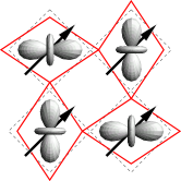
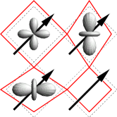
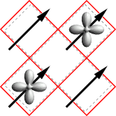
strong coupling

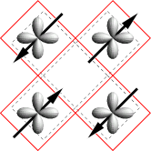
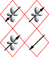
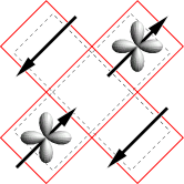
Figure 8: Schematic summary of the various spin, charge, orbital and lattice patterns calculated within the full model, Equation (27), at weak and strong electron phonon interaction and increasing doping.

Summarising the preceding sections, the complete microscopic model is given by

$$H=\sum_{i,\delta}R_{\delta}(H^{1,z}_{i,i+\delta}+H^{2,z}_{i,i+\delta})+H^{\rm EP}\,,$$ (27)

which contains all essential features of the low-energy physics of the manganites. The first term accounts for the ferromagnetic double-exchange interaction, which describes itinerant $e_{g}$ electrons that can optimise their kinetic energy by ordering the spin background formed out of localised $t_{2g}$ electrons. The second term couples this spin background to the orbital degrees of freedom of the $e_{g}$ electrons via Heisenberg type exchange interactions modulated by orbital projectors. It is thus responsible for anti-ferromagnetic phases, different orbital orderings as well as spin-orbital correlations. The third term, finally, causes all the polaronic effects and long range lattice distortions observed in some regions of the manganite phase diagram, but also affects the orbital ordering.

For analytical methods the above Hamiltonian is far too complex to be understood in full detail, and even its numerical solution is hard. Using high performance computers and new optimisation methods for the lattice degrees of freedom, we were able to study the ground-state properties of small clusters and to address, in particular, short range correlations [42, 43]. In Figures 5 to 8 we give a short overview of these results. The main features are the following: In the undoped compounds, e.g. LaMnO₃, only the second and third term of Equation (27) are active, and without electron phonon interaction the competition of the spin-orbital contributions depends sensitively on the values of the Coulomb and Hunds rule coupling $U$ and $J_{h}$, respectively. The dynamics of both subsystems is strongly correlated. With increasing electron phonon interaction the systems tends to develop static Jahn-Teller distortions, which also fix the orbital pattern and subsequently the spin order. Dynamic correlations of spins and orbitals are suppressed. Upon doping the ferromagnetic double-exchange comes into play, and only a substantial polaronic band narrowing due to strong electron lattice interaction can prevent ferromagnetic order. The orbital dynamics is coupled mainly to the charge dynamics, and is less affected by the spin-orbital terms (see Figure 6 where also the case $U=\infty$, i.e. the disabling of most of the spin-orbital terms, is considered). Interestingly, changes in the spin order are reflected also in the lattice fluctuations, an effect observed as well in experiment [31]. Facilitated by the electron lattice interaction at and above doping $x=0.5$ the susceptibility of the system to charge ordering dominates the low-energy behaviour and matching spin interactions lead to antiferromagnetic order. These features are, of course, well known from experiment [44, 45, 46]. The orbital correlations can show interesting patterns, involving, for instance, complex linear combinations $|\phi\rangle=\cos(\phi)|\theta\rangle+\sin(\phi)|\varepsilon\rangle$ of the $e_{g}$ states combined to two-site correlations proportional to $|\phi\rangle_{i}\otimes|\phi^{\prime}\rangle_{j}+|\phi^{\prime}\rangle_{i}\otimes|\phi\rangle_{j}$ with nonzero imaginary parts of $\phi$ and $\phi^{\prime}$. Similar complex correlations were also found in mean-field type treatments of the manganites [47, 48, 49].

Of course, numerical studies of small clusters are of limited value if we want to address long-range order or thermodynamic properties. For the former, mean-field studies of the complete microscopic model may give some insight and were carried out e.g. for the undoped compounds [26]. However, since a large number of ordering patterns usually differs by only tiny amounts of energy, the results of such calculations often depend on the underlying assumptions. The study of thermodynamic properties, on the other hand, requires further simplifications of the model, which will depend on the particular aspect of the manganite system that we are interested in. Hereafter we discuss some candidates of such simplified models.

One of the first models that was studied in connexion with the manganites is the double-exchange Hamiltonian [29, 30, 50],

$$\quad H^{\rm DE}=\frac{-t}{2S+1}\sum_{\langle ij\rangle,\sigma}\left(a_{i\sigma}^{\dagger}a_{j\sigma}\ c_{i}^{\dagger}c_{j}+{\rm H.c.}\right)\quad{\rm with}\quad\sum_{\sigma}a_{i\sigma}^{\dagger}a_{i}=2S+c_{i}^{\dagger}c_{i}\quad\forall i\,,$$ (28)

which follows from the first term in Equation (27) by omitting the orbital degrees of freedom and generalising to arbitrary on-site spin $S$. Despite its apparently simple structure – bosons coupled to spinless fermions – the model is not solvable directly, but many of its properties can been studied within the coherent potential approximation (CPA) [51, 52, 53] or, even more basic, by mean-field approximation [50]. The latter can be obtained by considering the matrix element for a single bond [30], $\tilde{t}=t(S_{T}+1/2)/(2S+1)$, and averaging over all orientations of the total bond spin $S_{T}$ within an effective mean field $\lambda=\beta g\mu_{B}H_{\rm eff}^{z}$ [50, 28]. The double-exchange model then reduces to the non-interacting fermion Hamiltonian

$$\qquad H_{\rm eff}^{\rm DE,1} =-t\ \gamma_{S}[S\lambda]\sum_{\langle ij\rangle}\left(c_{i}^{\dagger}c_{j}+{\rm H.c.}\right)\qquad{\rm with}$$ (29)

$$\qquad\gamma_{S}[S\lambda] =\frac{S+1}{2S+1}+\frac{\coth((S+1)\lambda)}{2}\left[\coth((S+1/2)\lambda)-\frac{\coth(\lambda/2)}{2S+1}\right]\,,{}$$

and for a given temperature the parameter $\lambda$ is chosen to minimise the free energy of the fermions and the spin system.

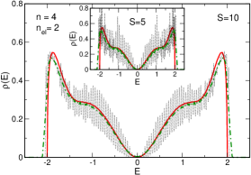
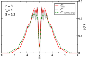
Figure 9: Density of non-zero eigenvalues of the quantum double-exchange model with spins of amplitude $S$ (dotted line: discrete spectrum; green dot-dashed line: running average) compared to the classical double-exchange model (bold red line). Left: Two fermions on a four site ring. Right: Four fermions on an eight site ring. See [28] for more details.

If the spin background is less important and the focus is more on the electrons and their interaction with other degrees of freedom (e.g. phonons, as discussed below), we may completely neglect the quantum nature of the spins. The most direct way to find the limit $S\to\infty$ of Equation (28) is the average over spin coherent states [54] which, for a classical spin background parameterised by the polar angles $\{\theta_{k},\phi_{k}\}$, yields [55, 56]

$$H_{\rm class}^{\rm DE} =-\sum_{\langle ij\rangle}\left(t_{ij}c_{i}^{\dagger}c_{j}+{\rm H.c.}\right)\qquad{\rm with}$$ (30)

$$t_{ij} =t\left[\cos\frac{\theta_{i}-\theta_{j}}{2}\cos\frac{\phi_{i}-\phi_{j}}{2}+i\,\cos\frac{\theta_{i}+\theta_{j}}{2}\sin\frac{\phi_{i}-\phi_{j}}{2}\right]\,.{}$$

To access the quality of this approximation, in a recent work [28] we calculated the density of states (DOS) of the double-exchange model for small finite systems and compared the cases of quantum and classical spins. As Figure 9 illustrates, at least in a disordered spin background the classical approximation describes the spectrum very well, even in the case $S=3/2$ that is relevant for the manganites.

In analogy to the mean-field model, Equation (29), where the spin background is taken into account only on average, we can also average over the fermion degrees of freedom to obtain an effective spin Hamiltonian. For the case of classical spins this leads to

$$H_{\rm eff}^{\rm DE,2}=-J_{\rm eff}\sum_{\langle ij\rangle}\sqrt{1+\vec{S}_{i}\vec{S}_{j}}\quad{\rm with}\quad J_{\rm eff}=t\,x(1-x)/\sqrt{2}\,.$$ (31)

Monte Carlo simulations [57, 58] show that the magnetisation data and critical temperatures of this model agree surprisingly well with those for the full classical double-exchange model [see Figure 10 (a)]. Summarising these different approximations we arrive at the conclusion that the double-exchange is well described by simple effective models, in particular, if we consider manganites with their almost classical spin amplitude $S=3/2$.

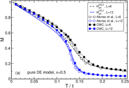
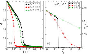
Figure 10: (a) Comparison of the magnetisation $M(T)$ of the classical double-exchange model, Equation (30), and of the effective model, Equation (31), obtained from Monte Carlo simulations [57, 58] of $L^{3}$ site clusters. (b) and (c) Suppression of the ferromagnetic order by electron phonon interaction; $\varepsilon_{p}=g^{2}/\omega$ denotes the coupling strength of the underlying Holstein double-exchange model. See [58] for more details.

As discussed above, the double-exchange interaction is responsible for the ferromagnetic metallic phase of the manganites. However, soon after the discovery of the colossal magneto-resistance effect additional electron-lattice interactions were realised to be important for an understanding of the conductivity [34, 35]. The third part of our complete model, $H^{\rm EP}$, contains three different phonon modes that couple to the orbital degrees of freedom or to the density, but certainly not all of them are equally important in different regions of the manganite phase diagram. For instance, matching the double-exchange model in Equation (28), we may again neglect orbital degrees of freedom and the corresponding phonon modes, which directly leads to the Holstein double-exchange model

$$\qquad H=\frac{-t}{2S+1}\sum_{\langle ij\rangle,\sigma}\left(a_{i\sigma}^{\dagger}a_{j\sigma}\ c_{i}^{\dagger}c_{j}+{\rm H.c.}\right)+g\sum_{i}(b_{i}^{\dagger}+b_{i})c_{i}^{\dagger}c_{i}+\omega\sum_{i}b_{i}^{\dagger}b_{i}\,.$$ (32)

Its properties have been studied with a number of methods and seem to account for many aspects of the metal-insulator transition and of the transport properties of ferromagnetic-metallic manganites with $0.25\lesssim x\lesssim 0.5$. A good overview is given e.g. in Ref. [59] with a focus on CPA. Analogous to the pure double-exchange Hamiltonian, we can also apply a number of further approximations to Equation (32), e.g. classical spins and phonons or Lang-Firsov type variational treatments of the lattice dynamics. In Figure 10 (b) and (c) we illustrate the suppression of ferromagnetic order by the electron-phonon interaction. To obtain these results the spin part of Equation (32) is approximated by the effective spin model from Equation (31) and the electron-phonon part is treated within a modified variational Lang-Firsov approximation [60, 61]. The resulting classical model is simulated with a Cluster Monte Carlo Method [58]. Finally note, that also the polaron problems related to $H^{\rm EP}$ are interesting by themselves. Neglecting the spin degrees of freedom, our full Hamiltonian (27) reduces to a fermionic hopping term plus electron phonon interactions of Holstein and $E\otimes e$ Jahn-Teller type. The corresponding few-fermion problems define the Holstein polaron and $E\otimes e$ Jahn-Teller polaron, whose properties have been studied numerically [62, 63].

Having discussed simplifications mainly of the double-exchange (first) and polaron (third) part of our microscopic model, we left out the spin-orbital (second) part so far. However, except for the various mean-field treatments, a further simplification, which does not alter the delicate balance of these degrees of freedom, is less obvious. On the one hand, there are a number of numerical studies [64, 65, 66] which focus on the orbital dynamics within a fixed spin background. On the other hand, we can study the interplay of spins and orbitals from a purely theoretical point of view and consider simplified models like that derived by Kugel and Khomskii [67]

$$H=J\sum_{\langle ij\rangle_{\delta}}\left[4({\bf S}_{i}{\bf S}_{j})(\tau^{\delta}_{i}+\frac{1}{2})(\tau^{\delta}_{j}+\frac{1}{2})+(\tau^{\delta}_{i}-\frac{1}{2})(\tau^{\delta}_{j}-\frac{1}{2})-1\right]\,,$$ (33)

where the orbital pseudo spin operators $\tau^{\delta}$ are related to our orbital projectors via $R_{\delta}(P^{\theta/\varepsilon})=1/2\pm\tau^{\delta}$. Recently, this model was considered in connexion to basic mechanisms of spin-orbital interaction, e.g. quantum disorder versus order-out-of-disorder [68, 69, 70]. Note also that there is a one-dimensional variant of the model, which is exactly solvable [71, 72].

7 Summary

In this contribution we focussed on a detailed introduction to the microscopic modelling of colossal magneto-resistance manganites, a class of materials which is particularly interesting due the close interplay of charge, spin, orbital and lattice degrees of freedom characterising its phase diagram and electronic properties. We supplemented the derivation by a discussion of various simplified models and their relation to our Hamiltonian. In addition, we reviewed some of our previous numerical results for the complete microscopic model and for its relatives.

References

References

- [1] Jonker G H and van Santen J H 1950 Physica 16 337
- [2] Wollan E O and Koehler W C 1955 Phys. Rev. 100 545
- [3] Kusters R M, Singleton J, Keen D A, McGreevy R and Hayes W 1989 Physica B 155 362
- [4] von Helmolt R, Wecker J, Holzapfel B, Schultz L and Samwer K 1993 Phys. Rev. Lett. 71 2331
- [5] Jin S, Tiefel T H, McCormack M, Fastnach R A, Ramesh R and Chen L H 1994 Science 264 413
- [6] Coey J M D, Viret M and von Molnár S 1999 Adv. Phys. 48 167
- [7] Tokura Y and Tomioka Y 1999 J. Magn. Magn. Mater. 200 1
- [8] Dagotto E, Hotta T and Moreo A 2001 Physics Reports 344 1
- [9] Moussa F, Hennion M, Rodríguez-Carvajal J, Moudden H, Pinsard L and Revcolevschi A 1996 Phys. Rev. B 54 15149
- [10] Urushibara A, Moritomo Y, Arima T, Asamitsu A, Kido G and Tokura Y 1995 Phys. Rev. B 51 14103
- [11] Rodríguez-Carvajal J, Hennion M, Moussa F, Moudden H, Pinsard L and Revcolevschi A 1998 Phys. Rev. B 57 R3189
- [12] Griffith J S 1971 The Theory of Transition-Metal Ions (Cambridge: Cambridge University Press)
- [13] Pickett W E and Singh D J 1996 Phys. Rev. B 53 1146
- [14] Satpathy S, Popović Z S and Vukajlović F R 1996 Phys. Rev. Lett. 76 960
- [15] Abbate M, de Groot F M F, Fuggle J C, Fujimori A, Strobel O, Lopez F, Domke M, Kaindl G, Sawatzky G A, Takano M, Takeda Y, Eisaki H and Uchida S 1992 Phys. Rev. B 46 4511
- [16] Chainani A, Mathew M and Sarma D D 1993 Phys. Rev. B 47 15397
- [17] Saitoh T, Bocquet A E, Mizokawa T, Namatame H, Fujimori A, Abbate M, Takeda Y and Takano M 1995 Phys. Rev. B 51 13942
- [18] Racah G 1942 Phys. Rev. 62 438
- [19] Condon E U and Shortley G H 1935 The Theory of Atomic Spectra (Cambridge: Cambridge University Press)
- [20] Bocquet A E, Mizokawa T, Saitoh T, Namatame H and Fujimori A 1992 Phys. Rev. B 46 3771
- [21] Tanabe Y and Sugano S 1954 J. Phys. Soc. Jpn. 9 766
- [22] Zaanen J and Sawatzky G A 1990 J. Solid State Chem. 88 8
- [23] Mizokawa T and Fujimori A 1995 Phys. Rev. B 51 12880
- [24] Quijada M, Černe J, Simpson J R, Drew H D, Ahn K H, Millis A J, Shreekala R, Ramesh R, Rajeswari M and Venkatesan T 1998 Phys. Rev. B 58 16093
- [25] Sarma D D, Shanthi N, Krishnakumar S R, Saitoh T, Mizokawa T, Sekiyama A, Kobayashi K, Fujimori A, Weschke E, Meier R, Kaindl G, Takeda Y and Takano M 1996 Phys. Rev. B 53 6873
- [26] Feiner L F and Oleś A M 1999 Phys. Rev. B 59 3295
- [27] Mattis D C 1988 The Theory of Magnetism I. Statics and Dynamics no. 17 in Springer Series in Solid-State Sciences (Heidelberg: Springer-Verlag)
- [28] Weiße A, Loos J and Fehske H 2001 Phys. Rev. B 64 054406
- [29] Zener C 1951 Phys. Rev. 82 403
- [30] Anderson P W and Hasegawa H 1955 Phys. Rev. 100 675
- [31] Booth C H, Bridges F, Kwei G H, Lawrence J M, Cornelius A L and Neumeier J J 1998 Phys. Rev. Lett. 80 853
- [32] Louca D, Egami T, Brosha E L, Röder H and Bishop A R 1997 Phys. Rev. B 56 R8475
- [33] Billinge S J L, Proffen T, Petkov V, Sarrao J L and Kycia S 2000 Phys. Rev. B 62 1203
- [34] Millis A J, Littlewood P B and Shraiman B I 1995 Phys. Rev. Lett. 74 5144
- [35] Millis A J 1998 Nature 392 147
- [36] Jahn H A and Teller E 1937 Proc. Roy. Soc. London, Ser. A 161 220
- [37] Jahn H A 1938 Proc. Roy. Soc. London, Ser. A 164 117
- [38] Longuet-Higgins H G, Öpik U, Pryce M H L and Sack R A 1958 Proc. Roy. Soc. London, Ser. A 244 1
- [39] Perlin Y E and Wagner M (eds.) 1984 The Dynamical Jahn-Teller Effect in Localized Systems no. 7 in Modern Problems in Condensed Matter Sciences (Amsterdam: North-Holland)
- [40] Holstein T 1959 Ann. Phys. (N.Y.) 8 325
- [41] Holstein T 1959 Ann. Phys. (N.Y.) 8 343
- [42] Weiße A and Fehske H 2002 Eur. Phys. J. B 30 487
- [43] Weiße A and Fehske H 2004 J. Magn. Magn. Mater. 272-276 92
- [44] Chen C H and Cheong S W 1996 Phys. Rev. Lett. 76 4042
- [45] Radaelli P G, Cox D E, Marezio M and Cheong S W 1997 Phys. Rev. B 55 3015
- [46] Renner C, Aeppli G, Kim B G, Soh Y A and Cheong S W 2002 Nature 416 518
- [47] Khomskii D 2000 Novel type of orbital ordering: complex orbitals in doped mott insulators URL http://arXiv.org/abs/cond-mat/0004034
- [48] van den Brink J and Khomskii D 2001 Phys. Rev. B 63 140416
- [49] Maezono R and Nagaosa N 2000 Phys. Rev. B 62 11576
- [50] Kubo K and Ohata N 1972 J. Phys. Soc. Jpn. 33 21
- [51] Kubo K 1972 J. Phys. Soc. Jpn. 33 929
- [52] Edwards D M, Green A C M and Kubo K 1999 J. Phys. Condens. Matter 11 2791
- [53] Green A C M and Edwards D M 1999 J. Phys. Condens. Matter 11 10511
- [54] Auerbach A 1994 Interacting Electrons and Quantum Magnetism Graduate Texts in Contemporary Physics (Heidelberg: Springer-Verlag)
- [55] Kogan E M and Auslender M I 1988 Phys. Status Solidi B 147 613
- [56] Müller-Hartmann E and Dagotto E 1996 Phys. Rev. B 54 R6819
- [57] Alonso J L, Fernández L A, Guinea F, Laliena V and Martín-Mayor V 2001 Nucl. Phys. B 596 587
- [58] Weiße A, Fehske H and Ihle D 2004 Spin-lattice coupling effects in the Holstein double-exchange model URL http://arXiv.org/abs/cond-mat/0406049 accepted for publication in Physica B
- [59] Edwards D M 2002 Adv. Phys. 51 1259
- [60] Lang I G and Firsov Y A 1962 Zh. Eksp. Teor. Fiz. 43 1843 [Sov. Phys. JETP 16, 1301 (1963)]
- [61] Fehske H 1996 Spin Dynamics, Charge Transport and Electron–Phonon Coupling Effects in Strongly Correlated Electron Systems Habilitationsschrift, Universität Bayreuth
- [62] Takada Y 2000 Phys. Rev. B 61 8631
- [63] El Shawish S, Bonča J, Ku L C and Trugman S A 2003 Phys. Rev. B 67 014301
- [64] Mack F and Horsch P 1999 Phys. Rev. Lett. 82 3160
- [65] van den Brink J, Horsch P, Mack F and Oleś A M 1999 Phys. Rev. B 59 6795
- [66] van den Brink J, Horsch P and Oleś A M 2000 Phys. Rev. Lett. 85 5174
- [67] Kugel K I and Khomskii D I 1973 Zh. Eksp. Teor. Fiz. 64 1429 [Sov. Phys. JETP 37, 725 (1973)]
- [68] Khaliullin G and Oudovenko V 1997 Phys. Rev. B 56 R14243
- [69] Feiner L F, Oleś A M and Zaanen J 1998 J. Phys. Condens. Matter 10 L555
- [70] Oleś A M, Feiner L F and Zaanen J 2000 Phys. Rev. B 61 6257
- [71] Uimin G V 1970 Zh. Eksp. Teor. Fiz. Pis’ma Red. 12 332 [JETP Lett. 12, 225 (1970)]
- [72] Itoi C, Qin S and Affleck I 2000 Phys. Rev. B 61 6747