Disorder Induced Transitions in Layered Coulomb Gases and Application to Flux Lattices in Superconductors

Abstract

A layered system of charges with logarithmic interaction parallel to the layers and random dipoles in each layer is studied via a variational method and an energy rationale. These methods reproduce the known phase diagram for a single layer where charges unbind by increasing either temperature or disorder, as well as a freezing first order transition within the ordered phase. Increasing interlayer coupling leads to successive transitions in which charge rods correlated in $N>1$ neighboring layers are unbounded by weaker disorder. Increasing disorder leads to transitions between different N phases. The method is applied to flux lattices in layered superconductors in the limit of vanishing Josephson coupling. The unbinding charges are point defects in the flux lattice, i.e. vacancies or interstitials. We show that short range disorder generates random dipoles for these defects. We predict and accurately locate a disorder-induced defect-unbinding transition with loss of superconducting order, upon increase of disorder. While $N=1$ charges dominate for most system parameters, we propose that in multi-layer superconductors defect rods can be realized.

I Introduction

There is considerable current interest in topological phase transitions induced by quenched disorder, a problem relevant for numerous physical systems. Such transitions are likely to shape the phase diagram of type II superconductors. It was proposed tgpldbragg that the flux lattice (FL) remains topologically ordered in a Bragg glass (BrG) phase at low field, and becomes unstable to the proliferation of dislocations above some threshold disorder (or field). The increased effect of disorder may lead to increased critical current, this providing one scenario for the ubiquitous and controversial ”second peak” Kes ; speakexp line in the phase diagram. Another scenario was proposed recently H2 and is based on a disorder-induced decoupling transition (DT) associated with the loss of superconducting order, responsible for a sharp drop in the FL tilt modulus. An important question then is whether this DT occurs before the BrG instability (i.e within the BrG phase) or whether both occur simultaneously.

Theoretically, two types of phase transitions were shown to be specific for pure layered superconductors. The first is decoupling GK ; Daemen ; H1 at which the Josephson coupling as well as the critical current between layers vanishes. The second is the proliferation of point ”pancake” vortices, vacancies and interstitials (VI) in the FL above a temperature $T_{def}$ which, above some field, is distinct from melting, as shown in the absence of Josephson coupling Dodgson . It is believed that this pure system topological transition merges with the decoupling transition Daemen ; H1 as the bare Josephson coupling is increased, being two anisotropic limits of the same transition H3 . This transition induces a loss of superconducting order (parallel to the layers by VI and perpendicular to them by the layer decoupling) while the positional correlations of the pure flux lattice is maintained FNF . This transition has also been studied in both limits in presence of point impurity disorder H1 ; HL as well as columnar disorder MHL . In particular, we have recently demonstrated HL the existence of disorder-induced, VI unbinding transition with loss of superconductivity in 3-dimensional (3D) layered superconductors, which would be particularly relevant to many layered superconductors and multilayer systems Kes ; Bruynseraede .

Topological phase transitions in two dimensional systems are conveniently studied using mapping onto Coulomb gases of charges interacting via a long range logarithmic potential. Studying general three dimensional systems, even for pure systems, is considerably more difficult. The limit of layered superconductors with magnetic coupling only, provides one rare example where the problem can be studied analytically in 3D in a controlled way. Indeed in this limit the problem amounts to coupled layers with 2D Coulomb interactions. In the presence of quenched disorder, the problem becomes quite subtle already in 2D because charges can freeze into inhomogeneous configurations. Progress was made recently and it was shown nattermann95 ; scheidl97 ; tang96 ; dcpld that quenched random dipoles lead to a phase transition, via proliferation of defects at a finite threshold value of disorder, even at temperature $T=0$. New analytical methods, based on RG for the charge fugacity probability distribution, and mapping onto a solvable model of directed polymer on the Cayley tree were developped in 2D tang96 ; dcpld . In a short account of the present work HL we have extended some of these techniques to study the 3D system in presence of disorder. Although a complete RG study along the lines of dcpld is possible in principle, we have used simpler, and we believe largely equivalent, methods. The first is an energy rationale which generalizes the Cayley tree mapping. Second, we have introduced HL a novel Gaussian variational method which incorporates the effect of the broad fugacity distribution, a feature previously revealed by the RG scheidl97 ; dcpld . This method was also applied to the single and two layer case in a related work on a random Dirac model relevant to quantum Hall systems rdirac .

The aim of this paper is to present details of our previous Letter HL focusing on two themes. First we consider a general Disordered Coupled Coulomb Gas (DCCG) model system defined by integer $\pm 1$ charges on $M$ layers in which the interaction

energy between two charges on layers $n$ and $n^{\prime}$ is $2J_{n-n^{\prime}}\ln r$ with $r$ the charge separation parallel to the layers; in addition the charges couple to quenched random dipoles. A general study of this system is performed both via an energy rationale and by a variational method, with consistent results. These methods are explained in detail. Second, we apply this study to various physical situations, mainly to layered superconductors in an external field. We justify, stating clearly the assumptions, that VI in the vortex lattice of layered superconductors with no Josephson coupling and in the presence of pinning disorder can be described by the DCCG model with quenched random dipoles.

In section II we present the DCCG model and its mapping to a sine-Gordon type problem. In section III we develop a $T=0$ energy rationale by an approximate mapping to Cayley tree problem. For the one layer case we find the well known critical disorder value of $\sigma_{cr}=1/8$ for the onset of VI. For the many layer case we find that as the anisotropy $\eta=-J_{1}/J_{0}$ increases a cascade of phase transitions appear at which the number of correlated charges on $N$ neighboring layers increases. These ”rod” phases appear at an decreasing critical disorder value until at $\eta\rightarrow 1/2$ we find $N\rightarrow\infty$ and $\sigma_{cr}\rightarrow 0$. In section IV we develop an efficient variational method which is tested on the one layer system, allowing for fugacity distributions, known dcpld to be important in 2D since disorder becomes broad at low temperature. We reproduce the phase boundary in disorder-temperature plane separating an ordered phase (bound charges) and a disordered (unbound charges, i.e. finite VI density); the critical disorder parameter at $T=0$ is $\sigma_{cr}=1/8$ is recovered. We also find a first order line within the ordered phase (seen in the dynamics study dcpld ) which becomes a crossover line in the disordered phase. In section V we extend our method to the 2-layer system and find for the anisotropy $\eta$ a critical value $\eta_{c}=1-1/\sqrt{2}$ above which the single layer type transition is preempted by a transition induced by bound states of two vortices on the two layers with $\sigma_{cr}<1/8$, in agreement with the energy rationale of section III. However, in a limited range of $1-1/\sqrt{2}<\eta<1/3$ we find coexistence with a two gap state, which is not captured by the energy rational in its simplest form, but does not change the value of $\sigma_{cr}$. Of course, all of these above results truly involve renormalized values of coupling $J_{n}^{ren}$ and disorder $\sigma^{ren}$. Although we have not attempted a full RG study, one main additional effect of RG is simply to substitute bare by renormalized values accounting for screening effects, which on the basis of the two layer case can be assumed to be small for our present purpose (i.e. identifying transition lines at low temperature).

In section VI we develop the effective theory of layered superconductors with magnetic coupling between layers, but without Josephson coupling. We show that point disorder for the FL leads to quenched dipoles for the VI, hence the DCCG problem. For typical layered superconductors we predict the one layer type transition with an effective disorder parameter. However, by increasing the separation between layers, as in multilayer systems Kes ; Bruynseraede to exceed the lattice parameter of the FL, one may realize the new $N>1$ rod phases.

II Model for disordered layered Coulomb gas

In this Section we define the model for $M$ coupled layers of disordered Coulomb gases and also in terms of an equivalent sine-Gordon model. Consider $n({\bf r},l)$ integer charges on the $l$-th layer at position ${\bf r}$ within the layer. The two-dimensional (2D) position ${\bf r}$ is defined on a lattice of spacing $\xi$, which for the superconducting system is the coherence length. We study the Hamiltonian:

$${\cal H}=-\frac{1}{2}\sum_{{\bf r}\neq{\bf r}^{\prime}}\sum_{l,l^{\prime}}2J_{ll^{\prime}}n({\bf r},l)G({\bf r}-{\bf r}^{\prime})n({\bf r}^{\prime},l^{\prime})-\sum_{{\bf r},l}V_{l}({\bf r})n({\bf r},l)+E_{c}\sum_{{\bf r},l}n^{2}({\bf r},l)$$ (1)

where $E_{c}$ is the core energy, accounting for short scale energies $r<\xi$. Charges on the same or different layers interact with a 2D Coulomb interaction, with

$$G({\bf r})\approx_{|{\bf r}|\to\infty}\ln\frac{|{\bf r}|}{\xi}\qquad G_{\bf q}\approx_{q\to 0}\frac{2\pi}{q^{2}}$$ (2)

with $G({\bf r})=\int_{\bf q}G_{{\bf q}}(1-e^{i{\bf q}.{\bf r}})$ and $\int_{\bf q}=\int\frac{d^{2}q}{(2\pi)^{2}}$ (on a square lattice $G_{{\bf q}}^{-1}=\frac{1}{\pi}[2-\cos(q_{x}\xi)-\cos(q_{y}\xi)]$). Neutrality is assumed in each layer. The disorder potential $V_{l}({\bf r})$ can be considered as due to random dipoles. A dipole has a potential $\sim 1/r$ or $\sim 1/q$ in Fourier space; hence the disorder potential on the $l$-th layer $V_{l}({\bf r})$ has long range correlations:

$$\overline{V_{l}({\bf q})V_{l^{\prime}}({\bf q}^{\prime})}\approx_{q\to 0}2\Delta_{ll^{\prime}}\frac{2\pi}{q^{2}}(2\pi)^{2}\delta^{(2)}({\bf q}+{\bf q}^{\prime})$$ (3)

$$\overline{(V_{l}({\bf r})-V_{l}({\bf r}^{\prime}))((V_{l^{\prime}}({\bf r})-V_{l^{\prime}}({\bf r}^{\prime}))}\approx_{|{\bf r}-{\bf r}^{\prime}|\to\infty}4\Delta_{ll^{\prime}}\ln\frac{|{\bf r}-{\bf r}^{\prime}|}{\xi}$$ (4)

where $\Delta_{ll^{\prime}}\geq 0$. This logarithmically correlated disorder is the one which exhibits a phase transition - other types of disorder with either weaker or stronger correlations result in either ordered or disordered phases, respectively, hence no phase transition as function of the disorder strength. One simpler case, which we will study in details, is the case of uncorrelated disorder from plane to plane, namely $\Delta_{ll^{\prime}}=\sigma J_{0}^{2}\delta_{ll^{\prime}}$. In that case one has

$$\overline{[V_{l}({\bf r})-V_{l}({\bf r}^{\prime})]^{2}}\approx_{|{\bf r}-{\bf r}^{\prime}|\to\infty}4\sigma J_{0}^{2}\ln\frac{|{\bf r}-{\bf r}^{\prime}|}{\xi}$$ (5)

It is clear that the model on a square lattice defined by its partition sum $Z_{\text{latt}}=\sum_{\{n({\bf r},l)\}}e^{-\beta H}$ can also be seen as a neutral 2D Coulomb gas model for $M$-component vector charges. A given configuration of charges is thus defined by a set of vector charges $\{n({\bf r},l)\}_{l=1,..M}$ on a 2D lattice.

We define the Fourier transform:

$$n({\bf q},k)=d\sum_{l}\sum_{\bf r}n({\bf r},l)e^{i{\bf q}\cdot{\bf r}+ikdl}$$ (6)

where d is the spacing between layers and in a continuum limit $d\sum_{l}\rightarrow\int dz$ and $\xi^{2}\sum\rightarrow\int d^{2}r$. The inverse formula for the charge density (per unit area) is

$$n({\bf r},l)/\xi^{2}=\int_{k}\int_{\bf q}n({\bf q},k)e^{-i{\bf q}\cdot{\bf r}-ikdl}$$ (7)

with $\int_{\bf q}=\int\frac{d^{2}q}{(2\pi)^{2}}$, $k=2\pi{\tilde{m}}/Md$ with ${\tilde{m}}$ integer, $-[M/2]+1\leq{\tilde{m}}\leq[M/2]$, and $\int_{k}=\frac{1}{Md}\sum_{k}\to\int_{-\pi/d}^{\pi/d}\frac{dk}{2\pi}$ at large $M$.

We perform disorder averages via the replica method, i.e. from the replicated partition function $\overline{Z^{m}}$ in the limit $m\to 0$, disorder averaged correlations and free energy are obtained. For integer $m$ we have

$$\overline{Z^{m}}=\sum_{\{n_{a}({\bf r},l)\}}e^{-\beta H^{(m)}}$$ (8)

with $\beta=1/T$, which on a lattice is exactly a Mm-component 2D vector Coulomb gas with integer charges at each site ${\bf r}$ with integer entries $n_{a}({\bf r},l)$ at each $a=1,..m$, $l=1,..M$. The replicated Hamiltonian is footnote0

$$\beta H^{(m)}=-\sum_{{\bf r}\neq{\bf r}^{\prime}}K_{la,l^{\prime}b}~{}n_{a}({\bf r},l)G({\bf r}-{\bf r}^{\prime})n_{b}({\bf r}^{\prime},l^{\prime})+\beta E_{c}\sum_{{\bf r},l,a}n^{2}_{a}({\bf r},l)$$ (9)

$$K_{la,l^{\prime}b}=\beta J_{ll^{\prime}}\delta_{ab}-\beta^{2}\Delta_{ll^{\prime}}$$ (10)

summation over repeated indices is assumed unless otherwise specified.

For system which is cyclic and (statistically) translationally invariant in the $z$ direction, i.e:

$$J_{ll^{\prime}}=J_{|l-l^{\prime}|}\qquad\Delta_{ll^{\prime}}=\Delta_{|l-l^{\prime}|}$$ (11)

it is convenient to work with a Fourier space version which reads:

$$\beta{\cal H}^{(m)}=\frac{1}{2d^{2}}\int_{k}\int_{q}n_{a}({\bf q},k)(G_{0})_{ab}({\bf q},k)n_{b}^{*}({\bf q},k)+\beta E_{c}\sum_{{\bf r},l,a}n^{2}_{a}({\bf r},l)$$ (12)

$$(G_{0})_{ab}({\bf q},k)=\frac{4\pi}{q^{2}}[g(k)\delta_{a,b}-\beta^{2}\Delta(k)]$$ (13)

For later convenience we have defined $g(k)=\beta J(k)$, $J(k)=d\sum_{l}J_{l}\exp(ikdl)$, with $J_{l}=\int_{k}J(k)\exp{-ikdl}$. Similarly $\Delta(k)=d\sum_{l}\Delta_{l,0}\exp(ikdl)$, i.e. for disorder uncorrelated between layers $\Delta(k)=d\sigma J_{0}^{2}$.

We proceed to define an equivalent sine-Gordon system. We first rewrite the logarithmic interaction by using a scalar field $\chi_{a}({\bf r},l)$,

$$\overline{Z^{m}}=\langle\sum_{\{n_{a}({\bf r},l)\}}\prod_{{\bf r},l,a}e^{-i\chi_{a}({\bf r},l)n_{a}({\bf r},l)-\beta E_{c}\sum_{{\bf r},l,a}n^{2}_{a}({\bf r},l)}\rangle_{\chi}$$ (14)

The average is done with the weight $\exp[-\frac{1}{2}\int_{k}\int_{q}\chi_{a}({\bf q},k)(G_{0}^{-1})_{ab}({\bf q},k)\chi^{*}_{b}({\bf q},k)]$; performing this Gaussian average one readily recovers Eq. (8). The inverse of Eq. (13) is derived by the inversion formula $(A\delta_{ab}+B)^{-1}=(1/A)\delta_{ab}-B/[A(A+Bm)]$, which for $m\to 0$ yields

$$(G_{0}^{-1})_{ab}({\bf q},k)=\frac{q^{2}}{4\pi}[\frac{1}{g(k)}\delta_{a,b}+\beta^{2}\frac{\Delta(k)}{g^{2}(k)}]\,.$$ (15)

The product in Eq. (14) at each lattice point ${\bf r}$ can be written as a sum of all $\pm 1,0$ values of $n_{a}({\bf r},l)$, i.e. a sum on all integer vector ${\bf n}=\{n_{a,l}\}$; $a=1,..m$, $l=1,..M$

$$\overline{Z^{m}}=\langle\prod_{{\bf r}}[1+\sum_{\{n\neq 0\}}Y[{\bf n}]e^{i\sum_{a,l}n_{a,l}\chi_{a}({\bf r},l)}]\rangle_{\chi}$$ (16)

where the fugacity is $Y[{\bf n}]=\exp[-\beta E_{c}\sum_{a,l}n^{2}_{a,l}]$. At this point we make an approximation of small fugacities $Y[{\bf n}]$ (dilute limit) and write the above as an exponent

$$\overline{Z^{m}}=\langle\prod_{{\bf r}}\exp[\sum_{\{n\neq 0\}}Y[{\bf n}]e^{i\sum_{a,l}n_{a,l}\chi_{a}({\bf r},l)}]\rangle_{\chi}\ \,.$$ (17)

This approximation neglects harmonics of $\exp[{\bf n}\cdot{\bf\chi}]$, i.e. it neglects vector charges with entries $|n_{a,l}|>1$. These harmonics are irrelevant near the actual phase transition dcpld . Here and below we define ${\bf n}\cdot{\bf\chi}=\sum_{la}n_{a,l}\chi_{a}({\bf r},l)$. The result Eq. (17) can now be identified as the partition sum for a sine-Gordon type Hamiltonian,

$$\beta{\cal H}_{SG}=\frac{1}{2}\int_{k}\int_{q}\chi_{a}({\bf q},k)(G_{0}^{-1})_{ab}({\bf q},k)\chi^{*}_{b}({\bf q},k)-\sum_{{\bf r}}\sum_{{\bf n}}Y[{\bf n}]\exp{i{\bf n}\cdot{\mbox{\boldmath$\chi$}}({\bf r})}\,.$$ (18)

where $\chi_{a}({\bf q},k)=\xi^{2}d\sum_{{\bf r}}\sum_{l}\chi_{a}({\bf r},l)e^{ikdl+i{\bf q}\cdot{\bf r}}$. We note that the $+$ sign for the off diagonal replica term in Eq. (15) corresponds to imaginary gauge disorder in a related Dirac problem rdirac . The validity of the approximations leading to (18) are discussed in dcpld in the context of a single layer. As also shown below, it is important, as done here, to retain replica charges with several non zero entries in order to describe the freezing transitions at low temperatures.

III energy rationale

In this section we consider the Coulomb gas problem at $T=0$ and develop an energy rationale to determine the phase diagram of the coupled layer system. The problem amounts to find minimal energy configurations of charges in a logarithmically correlated random potential. To ascertain the XY ordered phases (bound defects) and the transitions out of it (defect unbinding), a first step is to study the dilute limit of a single charge (or dipole). Even then, the full analytical solution is difficult, but various approximations have been argued to give exact leading order results. For a single layer it was studied either using nattermann95 ; korshunov_nattermann_diagphas ; castillo ; rem a “random energy model” (REM) approximation, or more accurately using a representation in terms of directed polymers on a Cayley tree (DPCT), introduced in tang96 ; chamon96 . The continuous version of the DPCT representation (branching process) was shown to emerge dcpld from the one loop Coulomb gas RG of the single layer problem, both for the single charge (or dipole) problem and for the many charges problem including screening effects. It is thus expected to be accurate.

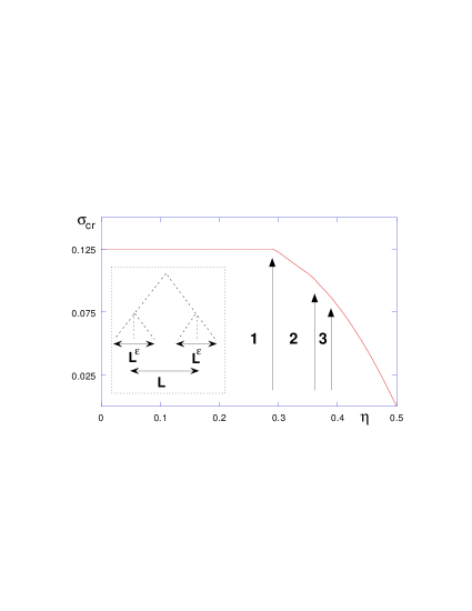
Schematically, one considers a tree with independent random potentials (Fig. 1 inset) $v_{i}$ on each bond with variance ${\bar{v}_{i}^{2}}=2\sigma J_{0}^{2}$. For definiteness we can discuss a tree of coordination $e^{2}$, the choice being immaterial for our present considerations. After $p$ generations one has $\sim e^{2p}$ sites which are mapped onto a 2D layer: each point ${\bf r}$ corresponds to a unique path on the tree with $v_{1},...,v_{p}$ potentials and is assigned a potential $V({\bf r})=v_{1}+...+v_{p}$. Two points ${\bf r}$, ${\bf r}^{\prime}$, separated by $|{\bf r}-{\bf r}^{\prime}|\sim e^{p^{\prime}}$ in Euclidean space, have a have a common ancestor at the previous $p^{\prime}\approx\ln|{\bf r}-{\bf r}^{\prime}|$ generation Since all bonds previous to the common ancestor are identical $\overline{[V({\bf r})-V({\bf r}^{\prime})]^{2}}=2\sum_{i=1}^{p}{\bar{v}_{i}^{2}}=4\sigma J_{0}^{2}\ln(|{\bf r}-{\bf r}^{\prime}|)$, reproducing Eq. (5) on each layer. Thus the growth of correlations on the tree and in Euclidean space is by construction the same, and the single charge problem corresponds to a single directed polymer. Exact solution of DPCT ct yields the best energy gained from disorder $V_{min}=min_{\bf r}V({\bf r})\approx-\sqrt{8\sigma}J_{0}\ln L$ for a volume $L^{2}$, with only $O(1)$ fluctuations dcpld , i.e $-\sqrt{8\sigma}J_{0}$ per generation $p=\ln L$. It is argued that this is also the exact result for the Euclidean problem. For a dipole in a single layer, one consider two directed polymers on the same Cayley tree. Opposite sign charge see opposite disorder $-v_{i}$, the gain from disorder $-V_{max}$ behaving identically. The configurations of the two oppositely charged polymers can however being argued to be essentially independent (i.e. determining maximum and minimum of a log-correlated landscape can be performed independently).

To generalize the Cayley tree argument we construct optimal energy charge configurations for $M$ coupled layers as follows. Consider $N$ neighboring layers with a $+,-$ pair on each layer and no charges on the other $M-N$ layers. We assume, for convenience, that $J_{0}>0$ and $J_{l\neq 0}\leq 0$ so that equal charges on different layers attract. The DPCT representation now involves on a single tree $N$ $+$ polymers (each seeing different disorder) and $N$ $-$ polymers (each seeing opposite disorder $-v_{i}$ to their $+$ partner). A plausible configuration is that the $+$ charges bind within a scale $L^{\epsilon}$ ($0\leq\epsilon\leq 1$), so do the $-$ charges, while the $+$ to $-$ charge separations define the scale $L$. Its tree representation (Fig. 1a) has $2N$ branches with $\epsilon\ln L$ generations, i.e. an optimal energy of $-2N\sqrt{8\sigma}J_{0}\epsilon\ln L$. On the scale between $L^{\epsilon}$ and $L$ the $+$ charges act as a single charge with a potential $\sum_{l=1}^{N}V_{l}({\bf r})$ (the $N$ polymers share the same branch) of variance $N\sigma$ hence the optimal energy is $-2\sqrt{8N\sigma}J_{0}(1-\epsilon)\ln L$. Note that the rod formation limits the disorder optimization leading to a disorder energy $\sim\sqrt{N}<N$. The total energy gain from the disorder potential is thus estimated as:

$$E_{dis}\approx-2J_{0}\sqrt{8\sigma}[\epsilon N+(1-\epsilon)\sqrt{N}]\ln L\,.$$ (19)

It is clearly exact for both $\epsilon=0$ and $\epsilon=1$, sufficient for our purpose. This result can also be obtained from the REM approximation, i.e. replacing the $V({\bf r})$ by $L^{2}$ variables uncorrelated in ${\bf r}$, with the same on-site variance $\overline{V^{2}({\bf r})}\sim 2\sigma J_{0}^{2}\ln L$ also yielding rem $V_{min}\sim-\sqrt{8\sigma}J_{0}\ln L$.

The competing interaction energy from the couplings $J_{l}$ is for the $+-$ pairs $[2J_{0}N+4\sum_{l=1}^{N}J_{l}(N-l)]\ln L$ while for the $++$ and $--$ pairs it is $-4\sum_{l=1}^{N}J_{l}(N-l)\epsilon\ln L$. Hence the interaction energy is

$$E_{int}=2J_{0}N[1-2\sum_{l=1}^{N}\eta_{l}(1-l/N)(1-\epsilon)]\ln L$$ (20)

where $\eta_{l}=-J_{l}/J_{0}$. The total energy $E_{tot}=E_{dis}+E_{int}$ is linear in $\epsilon$, hence the minimum is at either $\epsilon=1$ or at $\epsilon=0$. Since $\epsilon=1$ implies that the $+$ charges unbind, it is sufficient to consider $\epsilon=0$ with all $N\geq 1$, i.e. a rod is aligned with $N$ correlated charges at distance $O(1)$ and has energy

$$E_{tot}=2J_{0}N[1-2\sum_{l=1}^{N}\eta_{l}(1-\frac{l}{N})-\sqrt{\frac{8\sigma}{N}}]\ln L\,.$$ (21)

One can introduce more scales $L^{\epsilon^{\prime}}$ to describe the multi charges, however, as the energy is linear in $\epsilon^{\prime}$ the result is the same rod structure.

Figure 1: Critical disorder values with only nearest neighbor coupling $J_{1}$ vs. the anisotropy $\eta=-J_{1}/J_{0}$. Transitions between different $N$ phases are marked with arrows. Inset: the Cayley tree representation (for $N=3$ neighboring layers) with $+$ charges (at the tree endpoints) separated by $L^{\epsilon}$ along the layers, and separated by $L$ from the $N=3$ $-$ charges.

Consider first the case with only nearest neighbor coupling $\eta_{1}$ and only intralayer disorder correlation $\sigma J_{0}^{2}$. Disorder induces the $N$ vortex state (i.e. $E_{tot}$ vanishes) at the critical value

$$\sigma_{cr}^{(N)}=\frac{N}{8}[1-2\eta_{1}(1-\frac{1}{N})]^{2}\,.$$ (22)

The system is thus fully stable to disorder only for $\sigma<\sigma_{cr}$ with:

$$\sigma_{cr}=\min_{N}\frac{N}{8}[1-2\eta_{1}(1-\frac{1}{N})]^{2}\,.$$ (23)

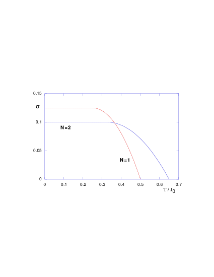
When $\sigma$ reaches $\sigma_{cr}$ the first instability is to one of the $N$ rod state, where $N$ depends on the value of the anisotropy $\eta_{1}$. If $\eta_{1}<\eta_{1}^{(1)}=1-1/\sqrt{2}$ then $\sigma_{cr}^{(N)}$ is minimal at $N=1$ and the first instability is similar to the one of a single layer with $\sigma_{cr}=1/8$. For larger anisotropies $\eta_{1}^{(N-1)}<\eta_{1}<\eta_{1}^{(N)}$, the first instability occurs at $\sigma_{cr}=\sigma_{cr}^{(N)}$ towards a $N$-rod state with $1/(1-2\eta_{1}^{(N)})=1+\sqrt{N(N+1)}\sim N$, thus with diverging $N$ as $\eta_{1}^{(N)}\to\frac{1}{2}$ (Fig 1) (for $\eta_{1}>\frac{1}{2}$ $E_{tot}<0$ even without disorder and the defects would form a lattice at $T=0$).

Upon increasing $\sigma$ beyond $\sigma_{cr}^{(N)}$ a given rod phase $N>1$ would eventually decompose into the $N=1$ phase. In particular the energies of the $N=1,2$ phases become equal at $\sigma_{cr}^{(1,2)}=\eta_{1}^{2}/[4(\sqrt{2}-1)^{2}]$ which equals 1/8 at $\eta_{1}=1-1/\sqrt{2}$. Hence at $\eta_{1}>1-1/\sqrt{2}$ the N=2 rods disintegrate into N=1 charges at $\sigma>\sigma_{cr}^{(1,2)}$. The variational solution (section VB) shows that this secondary line is actually at a somewhat lower $\sigma_{cr}^{(1,2)}$ (see Fig. 5 below).

In the general case with all couplings $J_{l}$ the critical value is:

$$\sigma_{cr}^{(N)}=\frac{N}{8}[1-2\sum_{l=1}^{N}\eta_{l}(1-\frac{l}{N})]^{2}\,.$$ (24)

We consider in particular $J_{l}$ with range of $l_{0}$ constrained by $\sum_{l}J_{l}=0$, as relevant for the superconductor system (section VI). An illustrative example is $\eta_{l}=\eta_{1}\exp(-(l-1)/l_{0})$, constrained as $\eta_{1}=\frac{1}{2}(1-\exp(-1/l_{0}))$ (note that $\sum_{l=1}^{N}\eta_{l}=\frac{1}{2}(1-\exp(-N/l_{0}))$. One then has:

$$\sigma_{cr}^{(N)}=\frac{1}{8N}\frac{(1-\exp(-N/l_{0}))^{2}}{(1-\exp(-1/l_{0}))^{2}}$$ (25)

For large $l_{0}\gg 1$, each $\eta_{l\neq 0}$ is small: $\sigma_{cr}^{(N)}$ as a function of $N$ starts by increasing and for $N\lesssim l_{0}$ the lowest $\sigma_{cr}^{(N)}$ is at $N=1$. However, the combined strength of $N\approx l_{0}$ vortices being significant, it has a maximum and then decreases back to zero for $N>l_{0}$ as $\sigma_{cr}^{(N)}\approx l_{0}^{2}/8N$. Hence $\sigma_{cr}^{(N)}\rightarrow 0$ as $N\rightarrow\infty$ and any small disorder seems to nucleate such vortices. This is because of the perfect screening of the zero mode $\sum_{l}J_{l}=0$ which implies that an infinite charge rod has a vanishing $\ln r$ interaction; hence a logarithmically correlated disorder is always dominant.

In practice, the realization of these large $N$ states depends, however, on the type of thermodynamic limit. Adding to Eq. (21) the core energy $2E_{c}N$ yields

$$E_{tot}^{\prime}=2J_{0}\sqrt{N}(\sqrt{8\sigma_{cr}^{(N)}}-\sqrt{8\sigma})\ln L+2E_{c}N$$ (26)

which becomes negative only beyond the scale

$$L_{N}\approx\exp\{E_{c}\sqrt{N}/[J_{0}(\sqrt{8\sigma}-\sqrt{8\sigma_{cr}^{(N)}})]\}\,.$$ (27)

This $L_{N}$ is the typical distance between rod vortices. Hence even if $\sigma>\sigma_{cr}^{(N)}$ only for system size $L>L_{N}$ the energy gain from disorder wins over core (and interaction) energy. Hence as $\sigma\rightarrow 0$ such states are only achievable in a thermodynamic limit where $L/N$ diverges exponentially. Using $\sigma_{cr}^{(N)}\approx l_{0}^{2}/8N$, for $N>l_{0}^{2}/8\sigma$ the lowest scale $L$ in this range is achieved at $N=l_{0}^{2}/2\sigma$ and leads to a (system size) lower bound $L_{min}\approx\exp[E_{c}l_{0}/4J_{0}\sigma]$ for observing large $N$ states with a given $\sigma<\frac{1}{8}$. For layered superconductors footnote1 $E_{c}/J_{0}\gg 1$ and $l_{0}\gg 1$ and this large $N$ instability occurs at unattainable scales, thus $N=1$ dominates. One needs $l_{0}\approx 2-3$ to realize the $N>1$ states, attainable in multilayers (see discussion section VII).

We finally generalize the energy argument for the $\epsilon=0$ configuration to the case of arbitrary correlations $\gamma_{l}=\Delta_{l}/\Delta_{0}$. The disorder energy can be found from the variance of $\sum_{i=1,N}V_{l}({\bf r})$ leading to the replacement $\sigma\to\sigma(1+2\sum_{l=1}^{N}(\Delta_{l,0}/\Delta_{0})(1-l/N))$ in Eq. (21). A more compact form can be obtained by writing directly

$$E_{tot}=2[\sum_{l=1}^{N}\sum_{l^{\prime}=1}^{N}J_{ll^{\prime}}-\sqrt{8\sum_{l=1}^{N}\sum_{l=1}^{N}\Delta_{ll^{\prime}}}]\ln L$$ (28)

Using that:

$$\sum_{l=1}^{N}\sum_{l^{\prime}=1}^{N}J_{ll^{\prime}}=\int_{k}J(k)\phi_{N}(k)$$ (29)

$$\phi_{N}(k)=\sum_{ll^{\prime}}^{N}e^{ikd(l-l^{\prime})}=\frac{\sin^{2}(Nkd/2)}{\sin^{2}(kd/2)}$$ (30)

One has the criticality condition for a $N$ rod:

$$\int_{k}\Delta(k)\phi_{N}(k)=\frac{1}{8}(\int_{k}J(k)\phi_{N}(k))^{2}$$ (31)

which in terms of $\sigma=\Delta_{0}/J_{0}^{2}$ has the critical value

$$\sigma_{cr}^{(N)}=\frac{1}{8}\frac{(\int_{k}\frac{\sin^{2}(Nkd/2)}{\sin^{2}(kd/2)}J(k)/J_{0})^{2}}{\int_{k}\frac{\sin^{2}(Nkd/2)}{\sin^{2}(kd/2)}\Delta(k)/\Delta_{0}}$$ (32)

For fixed anisotropies $J(k)/J_{0}$, $\Delta(k)/\Delta_{0}$ this relates the overall critical disorder strength $\sigma_{cr}^{(N)}$ to the rod length $N$.

IV variational method - the single layer

We develop here a variational method which allows for fugacity distributions, an essential feature in the one-layer problem. The method is developed in this section for the one-layer system and it is shown that one recovers in a simple way all the important known features for this problem. Furthermore, new insight is gained for a critical line within the ordered (charge bound) phase, as well as a crossover line in the disordered (charge unbound) phase, at which the the functional dependence of the charge density changes.

The single layer replicated Coulomb gas Hamiltonian is

$$\beta{\cal H}^{(m)}=\frac{1}{2}\int_{q}n_{a}({\bf q})\frac{4\pi}{q^{2}}[K\delta_{ab}-\sigma K^{2}]n_{b}^{*}({\bf q})+\beta E_{c}\sum_{{\bf r},a}n^{2}_{a}({\bf r})\,.$$ (33)

where $n_{a}({\bf q})=\sum_{\bf r}n_{a}({\bf r})e^{i{\bf q}\cdot{\bf r}}$. Note that $\sigma>0$ is here essential; the same 2D system with $\sigma<0$ has been shown to have a different phase diagram H4 ; scheidl98 . The equivalent sine-Gordon system is now

$$\beta{\cal H}_{SG}=\frac{1}{2}\int_{q}\chi_{a}({\bf q})(G_{0}^{-1})_{ab}(q)\chi^{*}_{b}({\bf q})-\sum_{{\bf r}}\sum_{{\bf n}}Y[{\bf n}]\exp{i{\bf n}\cdot{\mbox{\boldmath$\chi$}}({\bf r})}$$ (34)

$$(G_{0}^{-1})_{ab}(q)=\frac{q^{2}}{4\pi}[\frac{1}{K}\delta_{ab}+\sigma]$$ (35)

where $\chi_{a}({\bf q})=\xi^{2}\sum_{\bf r}\chi_{a}({\bf r})e^{i{\bf q}\cdot{\bf r}}$ and bare fugacities $Y[{\bf n}]=\exp(-\beta E_{c}\sum_{a}n_{a}^{2})$. Here one has simply ${\bf n}\cdot{\mbox{\boldmath$\chi$}}({\bf r})=\sum_{a}n_{a}\chi_{a}({\bf r})$, with ${\bf n}$ a nonzero vector with entries $n_{a}=\pm 1,0$.

The variational method represents the full Hamiltonian (34) by an optimal Gaussian one of the form

$$\beta{\cal H}_{var}=\frac{1}{2}\int_{q}G^{-1}_{ab}(q)\chi_{a}({\bf q})\chi_{b}(-{\bf q})$$ (36)

where $G_{ab}$ is to be determined by a variational principle. The variational free energy is $F_{var}=F_{0}+<{\cal H}_{SG}-{\cal H}_{var}>_{{\cal H}_{var}}$ with $\beta F_{0}=-\ln Z_{0}=-\frac{1}{2}Tr\ln G$ is found to read:

$$\frac{\beta F_{var}}{L^{2}}=-\frac{1}{2}\int_{q}Tr\ln G(q)+\frac{1}{2}\int_{q}Tr(G_{0}^{-1}(q)G(q))-\xi^{-2}\sum_{{\bf n}\neq 0}Y[{\bf n}]e^{-\frac{1}{2}\int_{q}{\bf n}\cdot G(q)\cdot{\bf n}}$$ (37)

up to an unimportant constant, where the $Tr$ is in replica indices. Taking the derivative $\frac{\delta}{\delta G_{ab}(q)}$ one obtains the saddle point equation:

$$\sigma_{ab}=\xi^{-2}\sum_{{\bf n}\neq 0}n_{a}n_{b}Y[{\bf n}]e^{-\frac{1}{2}{\bf n}\cdot G\cdot{\bf n}}$$ (38)

where we have defined:

$$G^{-1}_{ab}(q)=(G_{0})^{-1}_{ab}(q)+\sigma_{ab}$$ (39)

We recall first some technical relations scheidl97 ; dcpld . In the following we represent relevant operators as averages which depend only on $n_{+},n_{-}$, which are the number of $+$ or $-$ entries in ${\bf n}$, respectively. The averages have the form

$$A[{\bf n}]=\int dudv\Phi(u,v)e^{u(n_{+}+n_{-})+v(n_{+}-n_{-})}$$ (40)

where $z_{\pm}=e^{u\pm v}$ can be interpreted as fugacities for the $\pm$ charges, hence $\Phi(u,v)$ is a fugacity distribution. A sum on all ${\bf n}\neq 0$ can be written in terms of the variables $n_{+},n_{-}$ with a combinatorial factor for the number of ${\bf n}$ vectors with a given $n_{+},n_{-}$,

$$\lim_{m\to 0}\frac{1}{m}\sum_{{\bf n}\neq 0}A[{\bf n}]=\lim_{m\to 0}\frac{1}{m}\sum_{0<n_{+}+n_{-}\leq m}\frac{m!}{n_{+}!n_{-}!(m-n_{+}-n_{-})!}\langle e^{(u+v)n_{+}+(u-v)n_{-}}\rangle_{\Phi}$$ (41)

$$=\lim_{m\to 0}<(1+e^{u+v}+e^{u-v})^{m}/m>_{\Phi}=\langle\ln(1+e^{u+v}+e^{u-v})\rangle_{\Phi}$$ (42)

and the binomial expansion has been used and $<...>_{\Phi}$ denotes an average with the weight $\Phi(u,v)$. Similarly one has:

$$\lim_{m\to 0}\frac{1}{m}\sum_{{\bf n}\neq 0}\sum_{a}n_{a}^{2}A[{\bf n}]=\langle\sum_{{\bf n}\neq 0}(n_{+}+n_{-})e^{u(n_{+}+n_{-})+v(n_{+}-n_{-})}\rangle_{\Phi}$$

$$=\langle\partial_{u}\ln(1+e^{u+v}+e^{u-v})\rangle_{\Phi}=\langle\frac{e^{u+v}+e^{u-v}}{1+e^{u+v}+e^{u-v}}\rangle_{\Phi}$$ (43)

and

$$\lim_{m\to 0}\frac{1}{m}\sum_{{\bf n}\neq 0}\sum_{a,b}n_{a}n_{b}A[{\bf n}]=\langle\sum_{{\bf n}\neq 0}(n_{+}-n_{-})^{2}e^{u(n_{+}+n_{-})+v(n_{+}-n_{-})}\rangle_{\Phi}$$

$$=\langle\partial_{v}^{2}\ln(1+e^{u+v}+e^{u-v})\rangle_{\Phi}=\langle\frac{e^{u+v}+e^{u-v}+4e^{2u}}{(1+e^{u+v}+e^{u-v})^{2}}\rangle_{\Phi}$$ (44)

In our case we consider a replica symmetric parametrization $\sigma_{ab}=\sigma_{c}\delta_{ab}+\sigma_{0}$ so that $G_{ab}=\int_{q}G_{ab}(q)$ has the form $G_{ab}=G_{c}\delta_{ab}-A$, where

$$G_{c}=\int_{q}\frac{1}{\frac{q^{2}}{4\pi K}+\sigma_{c}}=K\ln\frac{\Lambda^{2}}{4\pi K\sigma_{c}}$$ (45)

$$A=\int_{q}\frac{\sigma_{0}+\frac{\sigma q^{2}}{4\pi}}{(\frac{q^{2}}{4\pi K}+\sigma_{c})^{2}}=K^{2}\sigma\ln\frac{\Lambda^{2}}{4\pi K\sigma_{c}}-K^{2}\sigma+\frac{K\sigma_{0}}{\sigma_{c}}$$ (46)

where $\Lambda\sim\xi^{-1}\gg K\sigma_{c}$ is a cutoff on the q integration. Since $\int_{q}{\bf n}\cdot G(q)\cdot{\bf n}=G_{c}\sum_{a}n_{a}^{2}-G(\sum_{a}n_{a})^{2}$ we can now identify the weight function from the interaction term in Eq. (37),

$$Y[{\bf n}]e^{-\frac{1}{2}\int_{q}{\bf n}\cdot G(q)\cdot{\bf n}}=e^{-(\frac{1}{2}G_{c}+\beta E_{c})(n_{+}+n_{-})+\frac{1}{2}A(n_{+}-n_{-})^{2}}$$

$$=\int dv\Phi(v)e^{u(n_{+}+n_{-})+v(n_{+}-n_{-})}$$ (47)

where here the weight function depends here only on $v$

$$\Phi(v)=\frac{1}{\sqrt{2\pi A}}e^{-v^{2}/(2A)}$$ (48)

and $u=-\beta E_{c}-\frac{1}{2}G_{c}$. We recall that:

$$y=e^{-\beta E_{c}}$$ (49)

is the bare fugacity of the charge, while the $z_{\pm}$ corresponds to the renormalized ones (they become random variables because of the quenched disorder in the system). The bare model can be generalized by introducing short-ranged randomness in the bare core energies (of width $E_{0}$) scheidl97 ; dcpld , resulting in the replica symmetric form $Y[{\bf n]}=\exp[-\beta E_{c}\sum_{a}n_{a}^{2}-\frac{1}{2}\beta^{2}E_{0}^{2}\sum_{ab}n_{a}n_{b}]$. This corresponds to the change $A\to A+\beta^{2}E_{0}^{2}$ in the averages above. Since A is divergent at criticality a finite $E_{0}$ can be ignored.

The interaction term in Eq. (37) is therefore

$$\sum_{{\bf n}\neq 0}Y[{\bf n}]e^{-\frac{1}{2}\int_{q}{\bf n}\cdot G(q)\cdot{\bf n}}=\langle\ln(1+e^{u+v}+e^{u-v})\rangle_{\Phi}$$ (50)

To identify $\sigma_{c},\sigma_{0}$ we consider the variational equation (38) and note that Eq. (IV) in the limit $m\to 0$ is $\sigma_{c}$, while Eq. (IV) is $\sigma_{c}+\sigma_{0}$, hence

$$\sigma_{c}=\xi^{-2}\langle\frac{e^{u+v}+e^{u-v}+4e^{2u}}{(1+e^{u+v}+e^{u-v})^{2}}\rangle_{\Phi}$$ (51)

$$\sigma_{0}=\xi^{-2}\langle\frac{(e^{u+v}-e^{u-v})^{2}}{(1+e^{u+v}+e^{u-v})^{2}}\rangle_{\Phi}\,.$$ (52)

These equations, together with (48) and (46) form the closed set of self-consistent equations that we want to solve. On general grounds one expects an ordered phase where the self energy $\sigma_{c}$ vanish corresponding to zero charge density and zero renormalized fugacity (XY phase). The solution with $\sigma_{c}>0$ corresponds to a phase with finite density of charges (disordered phase), the typical correlation length (see Eq. 39) being $\sim\sigma_{c}^{-1/2}$,the typicall distance between charges. We will thus perform the analysis near the critical line, where $\sigma_{c}$ is small. We will first neglect the $\sigma_{0}$ term in (46) and later show that it is indeed negligible in all regimes of interest.

To analyze these equations we note that the $v$ integration is dominated by large $|u|$ and $A$ which diverge at criticality, $\sigma_{c}\to 0$. The function displayed in (51) is maximal at $v=-u$ with a width $O(1)$, while the gaussian $\Phi(v)$ is maximal at $v=0$ with a width $O(\sqrt{A})$. Consider then $v>0$ where the $e^{u+v}$ term dominates and is either very small ($u+v<0$) or very large ($u+v>0$), hence

$$\xi^{2}\sigma_{c}\approx 2\int_{0}^{\infty}\frac{e^{u+v-v^{2}/2A}}{1+e^{u+v}}\frac{dv}{\sqrt{2\pi A}}\approx 2\int_{0}^{-u}e^{u+v-v^{2}/2A}\frac{dv}{\sqrt{2\pi A}}+2\int_{-u}^{\infty}e^{-u-v-v^{2}/2A}\frac{dv}{\sqrt{2\pi A}}\,.$$ (53)

In the second term the saddle point at $v=-A$ is outside of the integration range, hence it is dominated by the lower limit, i.e. it is of order $\exp(-u^{2}/2A)$. The first term has a saddle point at $v=A$ which is within the integration range if $A<-u$ and then

$$\sigma_{c}\sim e^{u+A/2}\sim y\sigma_{c}^{(K-K^{2}\sigma)/2}\qquad A<-u\,.$$ (54)

For $A<-u$ the second term of (53) is indeed smaller, $\exp(-u^{2}/2A)<\exp(u)\ll\exp(u+A/2)$. The range where $\sigma_{c}$ is finite, i.e. the charge density is finite and behaves as a plasma is where the exponent in the solution is positive (both $\sigma_{c}$ and $y$ being small),

$$\sigma_{c}\sim y^{\frac{2}{2-K+K^{2}\sigma}}\qquad K-K^{2}\sigma-2>0,\qquad\sigma<2/K^{2}$$ (55)

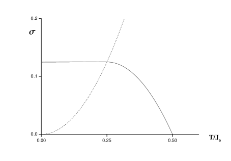
and the critical line where $\sigma_{c}$ vanishes is $K-K^{2}\sigma-2=0$ (Fig. 2); the condition $A<-u$ becomes $\sigma<2/K^{2}$ (see below). This is the first, or high temperature regime. In that regime a standard small fugacity expansion works, the effects of the width of $\Phi(v)$ are unimportant, both at the transition and in the disordered phase.

Considering now the second, or low temperature, regime $A>-u$. Then the first term of (53) is dominated by the upper limit, hence both terms of (53) yield

$$\sigma_{c}\sim e^{-u^{2}/2A}\sim y^{1/4K\sigma}\sigma_{c}^{1/8\sigma}\qquad\sigma>\frac{1}{8},\qquad A>-u\,.$$ (56)

Note that this corresponds to the distribution $\Phi(v)$ being very broad and then the maximum at $v=-u$ dominates the result. For the finite charge density phase we have now

$$\sigma_{c}\sim y^{\frac{2/K}{8\sigma-1}}\qquad\sigma>\frac{1}{8}\qquad\sigma>2/K^{2}$$ (57)

so that the critical line is $\sigma=\frac{1}{8}$ (Fig. 2); the condition $A>-u$ becomes $\sigma>2/K^{2}$ (see below).

Figure 2: Phase diagram for one layer in terms of $\sigma$ and $T/J_{0}=1/K$ variables. The full line is the defect transition given by $K-K^{2}\sigma-2=0$ at $\frac{1}{4}<1/K<\frac{1}{2}$ and by $\sigma=\frac{1}{8}$ at $1/K<\frac{1}{4}$. The dashed line $\sigma=2/K^{2}$ is a first order transition within the ordered (low $T$) phase while a crossover line in the disordered phase.

The boundary between the regimes (55) and (57) is $A=-u$, which for $\sigma_{c}\to 0$ is $\sigma=1/4K$, i.e. $\sigma=\frac{1}{8}$, $K=2$ on the critical line. The form (55) is then valid at high temperatures $K<2$ and a sum on single replica, single charge excitations is sufficient. In the low temperature regime ($K>2$), where Eq. (57) is valid, the summation on all charges in all replicas $n_{a}=(0,\pm 1)$ is essential in obtaining the correct result. It corresponds to the physics of the freezing, or prefered localisation of the charges in deep minima of the random potential.

It is instructive to evaluate the boundary between the regimes (55) and (57) for arbitrary small bare fugacity $y\ll 1$ also away from the critical line. The non-analytic behavior of the integral in Eq. (53) is related to the divergence of $u$, i.e. it exists in the ordered phase, while becomes a cross-over line in the disordered phase; this is further discussed below. Consider then a finite $\sigma_{c}$ and define $\sigma_{c}\sim y^{\gamma}$. For $y\ll 1$ the condition $A=-u$ becomes $\sigma=(1/2K)+(1/\gamma K^{2})$. For $A<-u$ we have from Eq. (55) $\gamma=2/(2-K+\sigma K^{2})$, hence the boundary is $\sigma=2/K^{2}$. Similarly, for $A>-u$, using $u=(K\gamma/2+1)\ln y$ yields $\gamma=(2/K)/(\sqrt{8\sigma}-1)$ and again the boundary is at $\sigma=2/K^{2}$. Hence there is a unique boundary between the two regimes [as included in the conditions for Eqs. (55) and (57)] which intersects the critical line at $\sigma=\frac{1}{8}$, $K=2$. The sharpness of this boundary, as mentioned above, depends on $\sigma_{c}\to 0$, hence in the disordered phase it depends on the smallness of $y$, i.e. it is a crossover line where the charge densities $\sim\sigma_{c}$ change from Eq. (55) to Eq. (57), a crossover whose width shrinks with $y$. In the ordered phase $\sigma_{c}=0$ and formally the boundary is sharp, although the relevant observable, i.e. the density, vanishes. One may still observe this transition by a finite size effect where the $q\to 0$ singularity is cutoff by the inverse area $1/L^{2}$ instead of $\sigma_{c}$, i.e. $\sigma_{c}\sim(1/L)^{K-\sigma K^{2}}$ or $\sim(1/L)^{1/4\sigma}$ in the two regimes, respectively. This transition is termed as a freezing transition; it is related to the single directed polymer transition on a Cayley tree ct , to a dynamic transition dcpld and also to a phase transition in a random gauge Dirac system rdirac .

Consider next $\sigma_{0}$, Eq. (52). The integral is again dominated by large $|v|$, hence

$$\sigma_{0}\approx\int_{0}^{\infty}\frac{e^{2u+2v}-v^{2}/2A}{(1+e^{u+v})^{2}}\frac{dv}{\sqrt{2\pi A}}\approx\int_{0}^{-u}e^{2u+2v-v^{2}/2A}\frac{dv}{\sqrt{2\pi A}}+\int_{-u}^{\infty}e^{-v^{2}/2A}\frac{dv}{\sqrt{2\pi A}}\,.$$ (58)

The second term is $\sim\exp(-u^{2}/2A)$ while the first term has a saddle point at $v=2A$ which is inside the integration range if $2A<-u$, and then

$$\sigma_{0}\sim y^{2}e^{2u+2A}\sim y^{2}(\sigma_{c})^{K-2\sigma K^{2}}\qquad\sigma<2/3K^{2}\,.$$ (59)

$2A<-u$ implies $\sigma<(1/4K)+1/(2\beta K^{2})$ and since also $A<-u$ we can use $\beta=2/(2-K+\sigma K^{2})$, hence $\sigma<2/3K^{2}$. Note that $\sigma_{0}\sim\sigma_{c}^{2-\sigma K^{2}}\ll\sigma_{c}$ when $\sigma<2/3K^{2}$, so that $\sigma_{0}/\sigma_{c}$ in Eq. (46) can be neglected. Consider next $2A>-u$ where the integrals for $\sigma_{0}$ are dominated by the end points $v=-u$. The range $-u<2A<-2u$ which corresponds to $2/3K^{2}<\sigma<2/K^{2}$ yields

$$\sigma_{0}\sim(\sigma_{c})^{(1+\sigma K^{2}/2)^{2}/(2\sigma K^{2})}\qquad 2/3K^{2}<\sigma<2/K^{2}$$ (60)

for which again $\sigma_{0}\ll\sigma_{c}$ while at $\sigma>2/K^{2}$ we have $\sigma_{0}\sim\sigma_{c}$. At $\sigma=2/3K^{2}$ the functional form of $\sigma_{0}$ changes, but since near this line $\sigma_{0}\ll\sigma_{c}$ there is no observable singularity.

To conclude, comparison with RG studies scheidl97 ; dcpld shows that the present variational method, which accounts for broad fugacity distributions, gives a remarkably accurate description of the transition and in particular of the freezing phenomena at low temperature in the single layer model. This is presumably because the screening effects (neglected in the variational approach) was shown, via higher order RG, to be very small at low temperature. In addition it provides a description of the disordered phase. The RG methods can be extended to many layers but following the joint distribution of the large set of random fugacities becomes rapidly difficult as $M$ increases. We thus now turn to the extension of the variational method to several layers.

V variational method - many layers

V.1 general case

We study now the full many-layer system, Eq. (18). We develop a variational method for $M$ coupled layers which allows for fugacity distributions, an essential feature in the one-layer problem. It is explicitly worked out for two layers, describing the various rod transitions as found by the energy rationale in section III, as well as a narrow transition region.

We note in particular the form of the interaction term $\exp{i{\bf n}\cdot{\mbox{\boldmath$\chi$}}({\bf r})}$; the naive approach would be to restrict to charges ${\bf n}$ with a single non zero entry, leading to a uniform fugacity term $-y\sum_{{\bf r},n,a}\cos({\mbox{\boldmath$\chi$}_{na}}({\bf r}))$ and a diagonal $k$-independent replica mass term. Instead we keep all composite charges ${\bf n}$, which allow for variational solutions with off diagonal and $k$-dependent replica mass terms. This corresponds respectively to fluctuations of fugacity and $N>1$ charge rods being generated and becoming relevant.

We note first that a rod solution is readily obtained from Eq. (12), i.e. we look for N correlated charge on nearest layers so that

$$|n_{a}({\bf q},k)|^{2}=|n_{a}({\bf q})d\sum_{l=0}^{N-1}e^{ikdl}|^{2}=d^{2}|n_{a}({\bf q})|^{2}\phi_{N}(k)$$ (61)

where $\phi_{N}(k)$ was defined in (30). With this replacement Eq. (12) has the form of a one-layer system Eq. (33) with effective parameters

$$K_{eff}=\int_{k}g(k)\phi_{N}(k)$$ (62)

$$\sigma_{eff}=\frac{\int_{k}\beta^{2}\Delta(k)\phi_{N}(k)}{(\int_{k}g(k)\phi_{N}(k))^{2}}$$ (63)

The system than has the same phase diagram as for one layer (Fig. 2) with these effective parameters. In particular the $T=0$ transition is at $\sigma_{eff}=\frac{1}{8}$, in agreement with Eq. (31).

We proceed with the variational scheme and define an optimal Gaussian Hamiltonian to approximate Eq. (18) as:

$${\cal H}_{0}=\frac{1}{2}\int_{k}\int_{\bf q}\chi_{a}({\bf q},k)G_{ab}({\bf q},k)\chi^{*}_{b}({\bf q},k)$$ (64)

$$G^{-1}_{ab}({\bf q},k))=(G_{0})^{-1}_{ab}({\bf q},k)+\sigma_{c}(k)\delta_{ab}+\sigma_{0}(k)$$ (65)

i.e the self energy can now depend on $k$.

The variational free energy is ${\cal F}_{var}={\cal F}_{0}+\langle{\cal H}_{SG}-{\cal H}_{0}\rangle_{0}$ where $\langle...\rangle$ is an average with respect to ${\cal H}_{0}$ and ${\cal F}_{0}$ is its free energy $\beta{\cal F}_{0}=-\frac{1}{2}Tr\ln G_{ab}({\bf q},k)$. The Gaussian average has the form

$$F[{\bf n}]\equiv\langle\exp{i{\bf n}\cdot{\mbox{\boldmath$\chi$}}({\bf r})}\rangle_{0}=\exp\{-\frac{1}{2}\int_{k}\sum_{a}|\sum_{l}n_{l,a}e^{ikdl}|^{2}G_{c}(k)+\frac{1}{2}\int_{k}|\sum_{l,a}n_{l,a}e^{ikdl}|^{2}A(k)\}$$ (66)

where we recall that $\int_{k}\equiv\frac{1}{Md}\sum_{k}$ and $\int_{q}G_{ab}(q,k)=G_{c}(k)\delta_{ab}-A(k)$, with

$$G_{c}(k)=\int_{q}G_{c}(q,k)=g(k)\ln[\Lambda^{2}/(4\pi g(k)\sigma_{c}(k))]$$

$$A(k)=\int_{q}G(q,k)=\beta^{2}\Delta(k)\ln[\Lambda^{2}/(4\pi g(k)\sigma_{c}(k))]-\beta^{2}\Delta(k)+g(k)\sigma_{0}(k)/\sigma_{c}(k)\,.$$ (67)

Extremization of $F_{var}$ yields the saddle point equation:

$$(\sigma_{c})_{ll^{\prime}}\delta_{ab}+(\sigma_{0})_{ll^{\prime}}=\xi^{-2}d^{-2}\sum_{{\bf n}}n_{al}n_{bl^{\prime}}Y[{\bf n}]F[{\bf n}]$$ (68)

since the dependence is on $l-l^{\prime}$, a corresponding Fourier transform yields

$$\sigma_{c}(k)\delta_{ab}+\sigma_{0}(k)=\xi^{-2}d^{-1}\sum_{{\bf n}}\sum_{l-l^{\prime}}n_{al}n_{bl^{\prime}}e^{ikd(l-l^{\prime})}Y[{\bf n}]F[{\bf n}]$$ (69)

We can now define $s_{a}(k)=d\sum_{l}n_{l,a}e^{ikdl}$. The $A(k)$ term can be written as an average over gaussian distributions of fugacities:

$$\prod_{k}\exp{(\frac{1}{2Md^{3}}|s_{a}(k)|^{2}A(k))}=\int\prod_{k}\frac{d^{2}w_{k}}{2\pi}\exp{(\frac{1}{Md^{2}}\sum_{k}\Re[\omega_{k}s_{a}^{*}(k)]-\frac{1}{2MA(k)d}|\omega_{k}|^{2})}$$ (70)

$$=\prod_{k}\langle\exp{(\frac{1}{Md^{2}}\Re[\omega_{k}s_{a}^{*}(k)])}\rangle_{\omega}$$ (71)

This form allows to decouple $\sum_{{\bf s}}F[{\bf s}]=\langle Z^{m}\rangle_{\omega}$ with

$$Z=\sum_{\{s_{n}=0,\pm 1\}}\exp(-\frac{1}{2d^{2}}\int_{k}\tilde{G}_{c}(k)|s(k)|^{2}+\frac{1}{d}\int_{k}\Re[\omega_{k}s^{*}(k)])$$ (72)

The variational equations for $m\rightarrow 0$ become

$$\sigma_{c}(k)=\xi^{-2}d\langle\frac{\partial^{2}\ln Z}{\partial\omega_{k}\partial\omega^{*}_{k}}\rangle_{\omega}\,;{\mbox{\hskip 5.69054pt}}\sigma_{0}(k)=\xi^{-2}d\langle|\frac{\partial\ln Z}{\partial\omega_{k}}|^{2}\rangle_{\omega}$$ (73)

We will not attempt to solve the general case but rather present a solution for $M=2$.

V.2 detailed solution for two layers

We consider now two layers with uncorrelated and equal disorder on each layer. The partition sum depends now on the number of $+$ and $-$ charges on each layer, i.e. on the 8 numbers $n_{\alpha,\beta}$ where $\alpha,\beta=\pm 1,0$, excluding $n_{00}$. For the vectors ${\bf n}_{1},{\bf n}_{2}$ in replica space for each layer, their number for a given collection of $n_{\alpha,\beta}$ is the combinatorial factor in the following sum

$$\sum_{{\bf n}_{1},{\bf n}_{2}}Y[{\bf n}_{1},{\bf n}_{2}]F[{\bf n}_{1},{\bf n}_{2}]= \sum_{n_{\alpha,\beta}}\frac{m!}{n_{00}!\,\,n_{+0}!...n_{++}!}\exp[-\beta E_{c}\sum_{a}(n_{a1}^{2}+n_{a2}^{2})-\frac{1}{4d}G_{c}(0)\sum_{a}(n_{a1}+n_{a2})^{2}$$ (74)

$$-\frac{1}{4d}G_{c}(\pi)\sum_{a}(n_{a1}-n_{a2})^{2}+\frac{1}{2}A_{1}(\sum_{a}n_{a1}+n_{a2})^{2}+\frac{1}{2}A_{2}(\sum_{a}n_{a1}-n_{a2})^{2}]$$

where $A_{1}=A(0)/2d$, $A_{2}=A(\pi)/2d$ and the sum is restricted to $\sum_{\alpha,\beta}n_{\alpha,\beta}=m$ . We need then two fugacity distributions,

$$\exp[\frac{1}{2}A_{i}(\sum_{a}n_{a1}\pm n_{a2})^{2}]=\int e^{\omega_{1}\sum_{a}(n_{a1}\pm n_{a2})}e^{-\omega_{i}^{2}/2A_{i}}\frac{d\omega_{i}}{\sqrt{2\pi A_{i}}}$$ (75)

where the upper (lower) signs corresponds to $i=1$ or $i=2$, respectively. The sum over $n_{\alpha,\beta}$ has the form of a ”ninomial” expansion, i.e. a power of 9 terms,

$$\sum_{{\bf n}_{1},{\bf n}_{2}}Y[{\bf n}_{1},{\bf n}_{2}]F[{\bf n}_{1},{\bf n}_{2}]=\langle Z^{m}\rangle_{\omega}$$ (76)

where the average is on both $\omega_{1}$, $\omega_{2}$. In terms of $u_{1}=-\frac{1}{2}\beta E_{c}-\frac{1}{4d}G_{c}(0)$ and $u_{2}=-\frac{1}{2}\beta E_{c}-\frac{1}{4d}G_{c}(\pi)$ we have

$$Z= 1+e^{u_{1}+u_{2}+\omega_{1}+\omega_{2}}+e^{u_{1}+u_{2}+\omega_{1}-\omega_{2}}+e^{u_{1}+u_{2}-\omega_{1}+\omega_{2}}+e^{u_{1}+u_{2}-\omega_{1}-\omega_{2}}$$ (77)

$$+e^{4u_{1}+2\omega_{1}}+e^{4u_{2}+2\omega_{2}}+e^{4u_{1}-2\omega_{1}}+e^{4u_{2}-2\omega_{2}}$$

The equations for the (dimensionless) self mass terms $\sigma_{c1}=\frac{\xi^{2}d}{2}\sigma_{c}(0)$, $\sigma_{c2}=\frac{\xi^{2}d}{2}\sigma_{c}(\pi)$ and similarly for $\sigma_{0i}$ are

$$\sigma_{ci}=<\frac{\partial^{2}\ln Z}{\partial\omega_{i}^{2}}>_{\omega}$$ (78)

$$\sigma_{0i}=<\frac{(\partial Z/\partial\omega_{i})^{2}}{Z^{2}}>_{\omega}\,.$$ (79)

These self masses correspond to length scales, i.e. $\sigma_{c1}^{-1/2}$ is the typical distance between ($++$) charge rods (i.e. a $+$ in layer 2 is on top of a $+$ in layer 1), while $\sigma_{c2}^{-1/2}$ is the typical distance between ($+-$) charge rods. In general $\sigma_{c2}\sim[\sigma_{c1}]^{\alpha}$ so that $\alpha=0$ corresponds to $\sigma_{c1}=0$ with N=2 ($+-$) rod defects, $\alpha=\infty$ corresponds to $\sigma_{c2}=0$ with N=2 ($++$) rod defects, $\alpha=1$ corresponds to the two length scales being equal hence an N=1 state, while other values of $\alpha$ imply the presence of two independent length scales.

A $N=2$ rod solution is readily obtained by $\sigma_{c2}=0$ so that $u_{2}\to\infty$ and $Z=1+e^{4u_{1}+2\omega_{1}}+e^{4u_{1}-2\omega_{1}}$. This is equivalent to the one layer system with

$$K_{eff}=2(K_{0}\pm K_{1})$$

$$\sigma_{eff}=\frac{\sigma K_{0}^{2}}{2(K_{0}\pm K_{1})^{2}}$$ (80)

where the lower sign corresponds to the $+,-$ rod solution $\sigma_{c1}=0$.

Consider now a general solution of the form $\sigma_{c2}\sim[\sigma_{c1}]^{\alpha}$ so that near criticality

$$u_{1}\to-\frac{1}{4}(K_{0}+K_{1})\ln(\Lambda^{2}/\sigma_{c1})\qquad A_{1}\to\frac{1}{2}\sigma K_{0}^{2}\ln(\Lambda^{2}/\sigma_{c1})$$

$$u_{2}\to-\frac{1}{4}\alpha(K_{0}-K_{1})\ln(\Lambda^{2}/\sigma_{c1})\qquad A_{2}\to\frac{1}{2}\alpha\sigma K_{0}^{2}\ln(\Lambda^{2}/\sigma_{c1})$$ (81)

Near criticality the $\omega$ integrals are dominated by large values so that positive and negative integration ranges are equivalent; furthermore, the $\omega_{1},\omega_{2}>0$ integral is dominated by exponents where $\omega_{1},\omega_{2}$ appear with positive sign,

$$\sigma_{c1}=\langle\frac{\partial}{\partial\omega_{1}}\frac{\partial Z/\partial\omega_{1}}{Z}\rangle_{\omega}\approx 4\langle\frac{\partial}{\partial\omega_{1}}\frac{e^{u_{1}+u_{2}+\omega_{1}+\omega_{2}}+2e^{4u_{1}+2\omega_{1}}}{1+e^{u_{1}+u_{2}+\omega_{1}+\omega_{2}}+e^{4u_{1}+2\omega_{1}}+e^{4u_{2}+2\omega_{2}}}\rangle_{\omega_{1},\omega_{2}>0}$$ (82)

We focus here on the low temperature behavior where $K_{i}\to\infty$ and the integrals are dominated by the maxima of the above $\partial/\partial\omega_{1}$. The fraction in Eq. (82) has values $0,1,2$ as indicated in Fig. 3 with boundaries shown by the full lines, assuming for now $u_{2}>u_{1}$ (the solution for $u_{2}<u_{1}$ can be inferred by the symmetry of the phase diagram under $K_{0},K_{1},\alpha\rightarrow K_{1},-K_{0},1/\alpha$). At the full lines in Fig. 3 $\partial/\partial\omega_{1}$ is maximal and dominate the integral at low temperatures since the Gaussian averaging factors are very flat. More precisely, we have separated the $\omega_{1}$ integral into ranges left and right of these lines and check in each range that it has no saddle point and is therefore dominated by $\omega_{1}$ at the line position. Thus for $\omega_{2}<-2u_{2}$ the integral is dominated by $\omega_{1}=-\omega_{2}-u_{1}-u_{2}$ leading to a contribution

$$\sigma_{c1}^{(1)}\sim\int_{0}^{-2u_{2}}d\omega_{2}e^{-(\omega_{2}+u_{1}+u_{2})^{2}/2A_{1}-\omega_{2}^{2}/2A_{2}}$$ (83)

while for $\omega_{2}>-2u_{2}$ the intgeral is dominated by $\omega_{1}=\omega_{2}+3u_{2}-u_{1}$ with the contribution

$$\sigma_{c1}^{(2)}\sim\int_{-2u_{2}}d\omega_{2}e^{-(\omega_{2}+3u_{2}-u_{1})^{2}/2A_{1}-\omega_{2}^{2}/2A_{2}}\,.$$ (84)

The saddle point of this integral is below $-2u_{2}$, hence it is dominated by $\omega_{2}=-2u_{2}$, i.e. is the same as $\sigma_{c1}^{(1)}$ if the latter is also dominated by $\omega_{2}=-2u_{2}$, or less than $\sigma_{c1}^{(1)}$ if the latter has a saddle point within the integration range. Hence $\sigma_{c1}^{(1)}$ determines the result with

$$\sigma_{c1}\sim e^{-(u_{1}+u_{2})^{2}/(2A_{1}+2A_{2})}\qquad(u_{2}-u_{1})A_{2}<-2u_{2}A_{1}$$

$$\sigma_{c1}\sim e^{-(u_{1}-u_{2})^{2}/(2A_{1})-2u_{2}^{2}/A_{2}}\qquad(u_{2}-u_{1})A_{2}>-2u_{2}A_{1}$$ (85)

Figure 3: Integration ranges for $\sigma_{c1}$ and $\sigma_{c2}$ when $u_{2}>u_{1}$ (i.e. $|u_{1}|>|u_{2}|$). For $\sigma_{c1}$ the numbers indicate the fraction value in Eq. (82) and the full lines are where the $\omega_{1}$ integral is dominant. For $\sigma_{c2}$ the numbers in parenthesis indicate the fraction value in Eq. (86) and the arrowed lines are where the $\omega_{2}$ integral is dominant.

Consider next $\sigma_{c2}$ which for $\omega_{1},\omega_{2}>0$ is dominated by

$$\sigma_{c2}=\langle\frac{\partial}{\partial\omega_{2}}\frac{\partial Z/\partial\omega_{2}}{Z}\rangle_{\omega}\approx 4\langle\frac{\partial}{\partial\omega_{2}}\frac{e^{u_{1}+u_{2}+\omega_{1}+\omega_{2}}+2e^{4u_{2}+2\omega_{2}}}{1+e^{u_{1}+u_{2}+\omega_{1}+\omega_{2}}+e^{4u_{1}+2\omega_{1}}+e^{4u_{2}+2\omega_{2}}}\rangle_{\omega_{1},\omega_{2}>0}\,.$$ (86)

The fraction above has values $0,1,2$ is indicated in Fig. 3 with boundaries shown by the arrowed lines; at these lines $\partial/\partial\omega_{2}$ is maximal and the corresponding $\omega_{2}$ dominate the integral. Hence for $\omega_{1}<u_{2}-u_{1}$ the integral is dominated by $\omega_{2}=-2u_{2}$ leading to a contribution

$$\sigma_{c2}^{(1)}\sim\int_{0}^{u_{2}-u_{1}}d\omega_{1}e^{-\omega_{1}^{2}/2A_{1}}e^{-2u_{2}^{2}/A_{2}}\sim e^{-2u_{2}^{2}/A_{2}}\,.$$ (87)

The next range is $u_{2}-u_{1}<\omega_{1}<-u_{2}-u_{1}$ where $\omega_{2}=-\omega_{1}-u_{1}-u_{2}$ dominates, contribution

$$\sigma_{c2}^{(2)}\sim\int_{u_{2}-u_{1}}^{-u_{2}-u_{1}}d\omega_{1}e^{-(\omega_{1}+u_{1}+u_{2})^{2}/2A_{2}}e^{-\omega_{1}^{2}/2A_{1}}\,.$$ (88)

This has a maximum within integration range if $(u_{2}-u_{1})A_{2}<-2u_{2}A_{1}$ with the result

$$\sigma_{c2}^{(2)}\sim e^{-(u_{1}+u_{2})^{2}/(2A_{1}+2A_{2})}\qquad(u_{2}-u_{1})A_{2}<-2u_{2}A_{1}$$ (89)

while if $(u_{2}-u_{1})A>-2u_{2}A_{1}$ the integral is dominated by its lower limit $u_{2}-u_{1}$ which is then always smaller then $\sigma_{c2}^{(2)}$. In the range $-u_{1}-u_{2}<\omega_{1}<-3u_{1}+u_{2}$ the line of maximum $\omega_{2}=\omega_{1}-3u_{2}+u_{1}$ is at large values of $\omega_{2}$ (see Fig. 3) so should give a small contribution; in fact integrating this line even from $u_{2}-u_{1}$ yields

$$\sigma_{c2}^{(3)}\sim\int_{u_{2}-u_{1}}d\omega_{1}e^{-(\omega_{1}+u_{1}-3u_{2})^{2}/2A_{2}}e^{-\omega_{1}^{2}/2A_{1}}\sim e^{-2u_{2}^{2}/A_{2}-(u_{2}-u_{1})^{2}/2A_{1}}$$ (90)

where the integrand has a maximum below the integration range and is therefore dominated by the lower integration limit. The result in Eq. (90) equals also to that of the integrand in (88) at its lower limit, hence $\sigma_{c2}^{(3)}\leq\sigma_{c2}^{(2)}$. Finally, the range $-3u_{1}+u_{2}<\omega_{1}$ has the line of maximum at $\omega_{2}=\omega_{1}+3u_{1}-u_{2}$, hence

$$\sigma_{c2}^{(4)}\sim\int_{-3u_{1}+u_{2}}d\omega_{1}e^{-(\omega_{1}+3u_{1}-u_{2})^{2}/2A_{2}}e^{-\omega_{1}^{2}/2A_{1}}\sim e^{-(3u_{1}-u_{2})^{2}/A_{1}}$$ (91)

where again the integral is dominated by its lower limit. This result is smaller then Eq. (89) (it is smaller then the integrand of (88) at $\omega_{1}=-u_{1}-u_{2}$, hence the latter is bigger if it has a maximum within integration range).

Figure 4: Two layer solutions for the exponent in $\sigma_{c2}\sim[\sigma_{c1}]^{\alpha}$ in terms of the anisotropy $\eta$. In the range $1-1/\sqrt{2}<\eta<1/3$ two solutions coexist.

Figure 5: The critical disorder $\sigma_{cr}$ for a two layer system. At $\eta<1-1/\sqrt{2}$ the transition is to a $N=1$ phase at $\sigma_{cr}=\frac{1}{8}$. For $\eta>1-1/\sqrt{2}$ at $\sigma_{cr}=\frac{1}{4}(1-\eta)^{2}$ the transition is either to an $N=2$ rod phase at $\eta>1/3$ or, for $1-1/\sqrt{2}<\eta<1/3$ a mixed phase $\sigma_{c2}\sim[\sigma_{c1}]^{\alpha}$ is possible. At $\eta>1/3$ the $N=2$ rod solution disintegrates into the $N=1$ phase at $\sigma_{cr}^{(1,2)}=(1+\eta)^{2}/16$.

Collecting all terms we have,

$$\sigma_{c2}\sim\max[e^{-2u_{2}^{2}},\,e^{-(u_{1}+u_{2})^{2}/(2A_{1}+2A_{2})}]\qquad(u_{2}-u_{1})A_{2}<-2u_{2}A_{1}$$ (92)

$$\sigma_{c2}\sim\max[e^{-2u_{2}^{2}},\,e^{-(3u_{1}-u_{2})^{2}/A_{1}}]\qquad(u_{2}-u_{1})A_{2}>-2u_{2}A_{1}\,.$$

Eqs. (V.2,92) can be written in terms of $\alpha$ and an anisotropy parameter $\eta=K_{1}/K_{0}>0$ (For $\eta<0$ we note that the solutions are symmetric under $\eta,\alpha\rightarrow-\eta,1/\alpha$). For $\eta<\frac{1+\alpha}{3+\alpha}$

$$\sigma_{c1} \sim[\sigma_{c1}]^{\frac{(1+\alpha+\eta-\eta\alpha)^{2}}{16(1+\alpha)\sigma}}$$

$$\sigma_{c2} \sim\max\{\,[\sigma_{c1}]^{\frac{\alpha(1-\eta)^{2}}{4\sigma}},\,\,[\sigma_{c1}]^{\frac{(1+\alpha+\eta-\eta\alpha)^{2}}{16(1+\alpha)\sigma}}\}$$ (93)

while for $\eta>\frac{1+\alpha}{3+\alpha}$ we have

$$\sigma_{c1} \sim[\sigma_{c1}]^{\frac{(1-\alpha+\eta+\eta\alpha)^{2}+4\alpha(1-\eta)^{2}}{16\sigma}}$$

$$\sigma_{c2} \sim\max\{\,[\sigma_{c1}]^{\frac{\alpha(1-\eta)^{2}}{4\sigma}}\,\,,[\sigma_{c1}]^{\frac{(3+3\eta-\alpha+\eta\alpha)^{2}}{16\sigma}}\}\,.$$ (94)

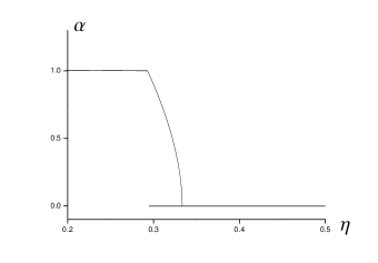
Some inspection shows that the latter equation has no solutions (except with $\alpha=0$, see below) while for Eq. (V.2) we have the following solutions (see Fig. 4): (i) The 2nd term of $\sigma_{c2}$ ($\sim\sigma_{c1}^{\alpha}$) identifies $\sigma_{c1}$ exponents and leads to $\alpha=1$ and criticality at $\sigma_{cr}=\frac{1}{8}$, i.e. the independent layer solution $N=1$. The 2nd term of the $\sigma_{c2}$ line is the maximal one if $\eta<1-1/\sqrt{2}$. (ii) The 1st term of $\sigma_{c2}$ identifies exponents as $(1-\eta)^{2}/4=(1+\alpha+\eta-\eta\alpha)^{2}/16(1+\alpha)$. This term dominates in the $\sigma_{c2}$ line if $\alpha<1$, hence the solution

$$\eta=\frac{2-\sqrt{1+\alpha}}{2+\frac{1-\alpha}{\sqrt{1+\alpha}}}$$ (95)

exists for $1-1/\sqrt{2}<\eta<1/3$ with $\sigma_{cr}=\frac{1}{4}(1-\eta)^{2}$. (iii) Finally $\alpha=0$ is possible, i.e. $\sigma_{c1}\equiv 0$ and an onset of just the $k=\pi$ component $\sigma_{c2}$. The solution is then of charges correlated between layers, i.e. the $N=2$ rod phase. Criticality is at $\sigma_{cr}=\frac{1}{4}(1-\eta)^{2}$, and from both Eqs. (V.2,V.2) this solution is valid at all $\eta$ provided it precedes the solution (i) with $\sigma_{cr}<\frac{1}{8}$, hence $\eta>1-1/\sqrt{2}$.

The solutions (i) and (iii) reproduce the energy rationale. We have found here an additional solution (ii) with a nontrivial new exponent $\alpha$ in a narrow range $1-1/\sqrt{2}<\eta<1/3$. This solution is a continuous interpolation in $\alpha$ between the $N=1$ solution ($\alpha=1$ at $\eta<1-1/\sqrt{2}$) and the $N=2$ rod solution ($\alpha=0$ at $\eta>1/3$). Both solutions (ii) and (iii) have the same $\sigma_{cr}$, hence they may be degenerate.

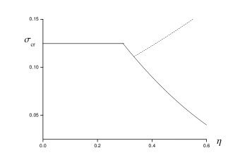
Solution (iii) allows for an additional phase transition corresponding to the onset of $\sigma_{c1}$, i.e. the $N=2$ rods decompose into independent $N=1$ charges on each layer. When $\sigma_{c2}\neq 0$, $u_{2}$ and $A_{2}$ are finite, hence the divergent terms in the exponent of Eq. (V.2) yield $\sigma_{c1}\sim e^{-u_{1}^{2}/2A_{1}}\sim\sigma_{c1}^{(1+\eta)^{2}/16\sigma}$, hence $\sigma_{cr}^{(1,2)}=(1+\eta)^{2}/16$ allows the onset of $\sigma_{c1}$ at $\eta>1/3$ (dashed line in Fig. 5). The energy rationale gives a somewhat higher $\sigma_{cr}^{(1,2)}=\eta_{1}^{2}/[4(\sqrt{2}-1)^{2}]$ for this $N=2$ to $N=1$ transition.

Figure 6: Phase diagram for the onset of the $N=1,2$ instabilities for anisotropy $\eta=0.35$. At low $T$ two distinct transitions are possible, the first being to the rod $N=2$ phase. At high $T$ the independent layer $N=1$ transition dominates and eliminates the $N=2$ phase.

Finally we consider the disorder-temperature phase diagram. The high temperature part of the phase boundary is determined by low order renormalization group as disorder is well behaved. Thus, in either Coulomb gas formulation dcpld or in sine-Gordon formulation we find the recursion with scale $\ell$

$$\frac{\partial Y[n]}{\partial\ell}=Y[n]\{2-\sum_{l,l^{\prime},a}n_{a,l}n_{a,l^{\prime}}K_{l-l^{\prime}}+\sigma K_{0}^{2}\sum_{l}[\sum_{a}n_{a,l}]^{2}\}$$ (96)

The $N=1$ solution is determined by one nonzero entry, hence $2-K_{0}+\sigma K_{0}^{2}=0$; for $N=2$ the solution corresponds to one nonzero entry per two layers, with the relative sign $\mp$, hence $2-2K_{0}\pm 2K_{1}+2\sigma K_{0}^{2}=0$. For $\eta>0$ the dominant transition (i.e. the one at lower temperature) has the upper sign, corresponding to $\sigma_{2c}$ with $k=\pi$. At $\sigma=0$ this has a critical temperature lower than that of $N=1$ since $K_{0}=1/(1-\eta)<2$ for $\eta<\frac{1}{2}$. Therefore the range of low $\sigma$ is dominated by the usual $N=1$ transition. In Fig. 6 we demonstrate the phase diagram with $\eta=0.35$ where the phases $N=1,2$ compete.

VI Application to superconductors

VI.1 Layered superconductor without disorder

The standard model for layered superconductors is the Lawrence Doniach model in terms of the superconducting phases on each layer and the electromagnetic vector potential. The latter can be integrated out H3 leading to an effective Hamiltonian in terms of pancake vortices, i.e. point singularities in each layer, and a nonsingular Josephson phase. We consider here the case without Josephson coupling, where the pancake vortices are not coupled to the Josephson phase. If $n({\bf r},l)$ is an integer field of $\pm 1,0$ corresponding to the location of pancake vortices then the vortex Hamiltonian is H3

$$H_{v}=\frac{1}{2}\sum_{{\bf r}\neq{\bf r}^{\prime}}\sum_{ll^{\prime}}n({\bf r},l)G_{v}({\bf r}-{\bf r}^{\prime},l-l^{\prime})n({\bf r}^{\prime},l^{\prime})+E_{c}\sum_{{\bf r},l}n({\bf r},l)^{2}\\$$ (97)

with:

$$G_{v}(q,k)=\frac{\Phi_{0}^{2}d^{2}}{4\pi\lambda_{ab}^{2}}\frac{1}{q^{2}}\frac{1}{1+f(q,k)}$$ (98)

$$f(q,k)=\frac{d}{4\lambda_{ab}^{2}q}\frac{\sinh(qd)}{\sinh^{2}(\frac{qd}{2})+sin^{2}(\frac{kd}{2})}$$ (99)

where $\lambda_{ab}$ is the magnetic penetration length parallel to the layers and $G_{v}(q,k)=d\sum_{l}\int d^{2}rG_{v}(r,l)e^{ikdl+i{\bf q}\cdot{\bf r}}$. The core energy is estimated as hu ; olive $E_{c}\approx(0.04-0.2)\tau$ where $\tau=\Phi_{0}^{2}d/(4\pi^{2}\lambda_{ab}^{2})$.

Note that the $k=0$ mode is screened, i.e. $G_{v}(q,k)$ is nonsingular at $q=0$. All the other modes are unscreened and lead to logarithmic interactions. This is because no screening current can go along $z$ (in the absence of Josephson coupling) and thus two pancakes in two different layers cannot screen each others.

In presence of an external field $B$ along $z$ a flux lattice with a unit cell area $a^{2}=\Phi_{0}/B$ is formed. The flux lattice is composed of pancake vortices, i.e. point singularities, which are displaced from the $p$-th line position ${\bf R}_{p}$ at the $l$-th layer into ${\bf R}_{p}+{\bf u}_{p}^{l}$; its Fourier transform is

$${\bf u}({\bf q},k)=da^{2}\sum_{l}\sum_{p}{\bf u}_{p}^{l}e^{i{\bf q}\cdot{\bf R}_{p}+ikdl}$$ (100)

Expanding Eq. (97) to second order in ${\bf u}_{p}^{l}$ yields the elastic Hamiltonian of the form,

$$H_{el}=\frac{1}{2}\int_{k}\int_{{\bf q}}[D_{L}(q,k)|u_{L}({\bf q},k)|^{2}+D_{T}(q,k)|u_{T}({\bf q},k)|^{2}]\,.$$ (101)

We will be mainly interested in the case of no Josephson coupling, where the following exact expression holds:

$$D_{L}(q,k)P^{L}_{\alpha\beta}(q)+D_{T}(q,k)P^{T}_{\alpha\beta}(q)$$ (102)

$$=\frac{1}{a^{4}d^{2}}(q_{\alpha}q_{\beta}G_{v}(q,k)+\sum_{Q\neq 0}((Q+q)_{\alpha}(Q+q)_{\beta}G_{v}(Q+q,k)-Q_{\alpha}Q_{\beta}G_{v}(Q,0)))$$ (103)

provided we add a short distance cutoff in plane, i.e replace $G_{v}(q,k)\to G_{v}(q,k)e^{-q^{2}\xi^{2}/2}$. The conventional elastic moduli are then identified as:

$$D_{L}(q,k)=q^{2}c_{11}(q,k)+k_{z}^{2}c_{44}^{L}(q,k)$$ (104)

$$D_{T}(q,k)=q^{2}c_{66}(q,k)+k_{z}^{2}c_{44}^{T}(q,k)$$ (105)

where $k_{z}^{2}=\frac{4}{d^{2}}sin^{2}(\frac{kd}{2})$. For zero Josephson coupling it is found Goldin , where leading terms in $q^{2}$ are retained,

$$c_{66}(q,k)=\frac{B\Phi_{0}}{(8\pi\lambda_{ab})^{2}}$$ (106)

$$c_{11}(q,k)+c_{66}(q,k)=\frac{B^{2}}{4\pi}\frac{1}{1+\lambda_{ab}^{2}(q^{2}+k_{z}^{2})}$$ (107)

$$c_{44}^{L}(q,k)=\frac{B^{2}}{4\pi}\frac{1}{1+\lambda_{ab}^{2}(q^{2}+k_{z}^{2})}+c_{44}^{T}(k)$$ (108)

$$c_{44}^{T}(k)=\frac{1}{2}(\frac{1}{da^{2}})^{2}\frac{1}{k_{z}^{2}}\sum_{{\bf Q}\neq{\bf 0}}(G_{v}(Q,k)-G_{v}(Q,0))Q^{2}\approx\frac{2B\Phi_{0}}{(8\pi\lambda_{ab}^{2})^{2}}\frac{1}{k_{z}^{2}}\ln\frac{1+k_{z}^{2}/Q_{0}^{2}}{1+\xi^{2}k_{z}^{2}}$$ (109)

and the last form is in the limit $d\ll a,\lambda_{ab}$. We note that with Josephson coupling the results for $c_{66},c_{11}$ are unchanged, while $c_{44}^{L,T}$ are modified with a stronger effect Goldin on $c_{44}^{T}$.

We consider first the defect transition in the pure system Dodgson . This refers to the proliferation of vacancy interstitial pairs (VI), thereby destroying the superconducting order parallel to the layers. These defects correspond to additional pancake vortices, denoted by $s_{l}({\bf r})$ on top of the ones forming the flux lattice. These defects couple to the lattice via the same coupling of Eq. (97),

$${\cal H}_{vac}=\sum_{{\bf r},p,l,l^{\prime}}s_{l}({\bf r})G_{v}({\bf R}_{p}+{\bf u}_{p}^{l^{\prime}}-{\bf r},l-l^{\prime})$$ (110)

To 0-th order in ${\bf u}_{l}^{n}$ the defects feel a periodic potential:

$${\cal H}_{vac}^{(0)}=\sum_{{\bf r},p,l,l^{\prime}}s_{l}({\bf r})G_{v}({\bf R}_{p}-{\bf r},l-l^{\prime})$$ (111)

which fixes the defect position in a unit cell, hence fluctuations of $s({\bf q},k)=d\sum_{l}\sum_{\bf r}s_{l}({\bf r})e^{ikdl+i{\bf q}\cdot{\bf r}}$ involve only ${\bf q}$ in the first Brillouin zone (BZ); in the following (and in Eq. 101) all $q$ integrals are restricted to the first BZ. Note that for vacancies the periodic potential has minima on the flux lines, while for interstitials the minima are in the middle of the unit cell. Hence, the core energies of vacancies and interstitials differ, but as they come in pairs, $E_{c}$ refers to an average of these core energies. For an isolated pancake vortex hu $E_{c}\approx(0.1-0.2)\tau$, while in presence of a flux lattice with local relaxation leads to olive $E_{c}\approx 0.04\tau$.

Expanding to first order, one finds with the above definitions:

$${\cal H}_{vac}(s,u)={\cal H}_{vac}^{(0)}(s)+{\cal H}_{vac}^{(1)}(s,u)+O(su^{2})$$ (112)

$${\cal H}_{vac}^{(1)}(s,u)=\frac{1}{a^{2}d^{2}}\int_{k}\int_{q}s({\bf q},k)G_{v}(q,k)(-i{\bf q})\cdot{\bf u}(-{\bf q},-k)$$ (113)

The total energy is thus:

$$H_{el}(u)+{\cal H}_{vac}^{(1)}(s,u)+{\cal H}_{v}(s)=\frac{1}{2}\int_{k}\int_{q}D_{T}(q,k)|u_{T}({\bf q},k)|^{2}$$ (114)

$$+\frac{1}{2}\int_{k}\int_{q}[(D_{L}(q,k)|u_{L}({\bf q},k)|^{2}+\frac{1}{d^{2}}s({\bf q},k)G_{v}(q,k)s(-{\bf q},-k)+\frac{2}{a^{2}d^{2}}s({\bf q},k)G_{v}(q,k)(-iq)u_{L}(-{\bf q},-k)]$$ (115)

One can either minimize it to find the (purely longitudinal) deformation of the lattice induced by the defect,

$${\bf u}_{vac}({\bf q},k)=i{\bf q}s({\bf q},k)G_{v}(q,k)/a^{2}d^{2}D_{L}(q,k)$$ (116)

and compute ${\cal H}_{el}+{\cal H}_{vac}+{\cal H}_{v}$ at the minimum or, since it is Gaussian, simply integrate out the displacements $u_{L}({\bf q},k)$. One finds that the screening of the vortices by the longitudinal displacements of the lattice results in an effective interaction energy between the defects:

$${\cal H}^{eff}_{v}(s)=\frac{1}{2d^{2}}\int_{k}\int_{q}s({\bf q},k)G^{eff}_{v}(q,k)s(-{\bf q},-k)$$ (117)

$$G^{eff}_{v}(q,k)=G_{v}(q,k)(1-\frac{q^{2}G_{v}(q,k)}{a^{4}d^{2}D_{L}(q,k)})$$ (118)

One can connect with the notations of the previous sections ($\beta=1/k_{B}T$):

$$g(k)=\frac{\beta}{4\pi}\lim_{q\to 0}q^{2}G^{eff}_{v}(q,k)$$ (119)

The pure defect transition thus occurs when:

$$K_{eff}=\int_{k}g(k)=2\quad\leftrightarrow\quad T_{def}=\frac{1}{8\pi}\int_{k}G^{eff}_{v}(k)$$ (120)

where we define:

$$G_{v}(k)=\lim_{q\to 0}[q^{2}G_{v}(q,k)]=\frac{\Phi_{0}^{2}d^{2}}{4\pi}\frac{k_{z}^{2}}{1+\lambda_{ab}^{2}k_{z}^{2}}$$ (121)

$$G^{eff}_{v}(k)=\lim_{q\to 0}[q^{2}G^{eff}_{v}(q,k)]=G_{v}(k)(1-\frac{G_{v}(k)}{a^{4}d^{2}D_{L}(0,k)})$$ (122)

where we recall $k_{z}^{2}=\frac{4}{d^{2}}sin^{2}(\frac{kd}{2})$.

It is instructive to consider the ”unscreened defect transition” temperature, i.e. formation of pancake vortices in the absence of an external field. This is denoted as the vortex transition H3 with the onset temperature at

$$T_{v}=\frac{1}{8\pi}\int_{k}G_{v}(k)=\frac{\Phi_{0}^{2}d}{2(4\pi\lambda_{ab})^{2}}h(d/(2\lambda_{ab}))$$ (123)

$$h(y)=\frac{1}{2\pi}\int_{-\pi}^{\pi}dx\frac{1}{1+\frac{y^{2}}{sin^{2}(\frac{x}{2})}}=1-\frac{y}{\sqrt{1+y^{2}}}$$ (124)

In particular for $d\ll\lambda$ one has:

$$T_{v}\approx\frac{\Phi_{0}^{2}d}{2(4\pi\lambda_{ab})^{2}}=\tau/8\,.$$ (125)

The actual superconducting transition is at $T_{c}$ with $T_{v}<T_{c}<T_{f}$ where $T_{f}$ is the fluxon transition temperature, where Josephson decoupling would occur in the absence of pancake defects H3 .

To compare the vortex transition with melting we use a Lindemann type criterion (with only transverse modes).

$$c_{L}^{2}a^{2}=\langle u^{2}\rangle=T_{m}\int_{k}\int_{q,BZ}\frac{1}{c_{66}q^{2}+c_{44}^{T}k_{z}^{2}}=\frac{T_{m}}{4\pi c_{66}}\int_{k}\ln(1+\frac{4\pi c_{66}}{c_{44}^{T}a^{2}k_{z}^{2}})$$ (126)

Using a circular BZ of volume $(2\pi/a)^{2}$, hence $0<q^{2}<4\pi/a^{2}$,

$$T_{m}\approx\frac{4\pi c_{L}^{2}}{A}c_{66}a^{2}d=\frac{4\pi c_{L}^{2}}{A}\frac{\Phi_{0}^{2}d}{(8\pi\lambda_{ab})^{2}}$$

$$A=d\int_{k}\ln(1+\frac{4\pi c_{66}}{c_{44}^{T}a^{2}k_{z}^{2}})=d\int_{k}\ln(1+\frac{\phi_{0}^{2}}{16\pi a^{4}\lambda^{2}D_{T}(0,k)})$$ (127)

where in the last equation we have used the dispersionless value of $c_{66}$ valid for $a\gg d$. The scales of the vortex and melting transitions are the same, their ratio being $T^{0}_{def}/T_{m}=A/4\pi c_{L}^{2}$. Hence the condition that the defect transition occurs before melting and can thus be consistently described is that $G^{eff}_{v}(q,k)\ll G_{v}(q,k)$.

Let us now study the true transition with screening. One denotes $D_{L,T}(k)=D_{L,T}(0,k)=k_{z}^{2}c_{44}^{L,T}(0,k)$ respectively. Using the above result, one finds in the $q\to 0$ limit the exact expressions:

$$D_{T}(k)=\frac{1}{2}(\frac{1}{da^{2}})^{2}\sum_{{\bf Q}\neq{\bf 0}}(G_{v}(Q,k)-G_{v}(Q,0))Q^{2}$$ (128)

$$D_{L}(k)=D_{T}(k)+\frac{1}{a^{4}d^{2}}G_{v}(k)$$ (129)

One thus has:

$$G_{v}^{eff}(k)=G_{v}(k)\frac{D_{T}(k)}{D_{L}(k)}=\frac{\Phi_{0}^{2}d^{2}}{4\pi}\frac{k_{z}^{2}}{1+\lambda_{ab}^{2}k_{z}^{2}}\frac{\epsilon(k)}{1+\epsilon(k)}$$ (130)

$$\epsilon(k)=a^{4}d^{2}D_{T}(k)/G_{v}(k)\,.$$ (131)

Hence the condition for $T_{def}\ll T_{m}$, which justifies our description of the defect transition, is $\epsilon(k)\ll 1$. We note also that for a single 2D layer there is no tilt modulus for the FL and $\epsilon=0$; hence a 2D FL has VI’s at any finite temperature.

Let us first consider the regime $2\pi d\ll a<\lambda$ relevant for layered superconductors. As shown in the Appendix one has in this regime:

$$D_{T}(k)\approx\frac{\Phi_{0}^{2}}{32\pi^{2}\lambda_{ab}^{4}a^{2}}\ln\frac{1+k_{z}^{2}/Q_{0}^{2}}{1+{\bar{d}}^{2}k_{z}^{2}}+\frac{\Phi_{0}^{2}d^{2}}{8Q_{0}^{2}a^{4}\lambda_{ab}^{4}}k_{z}^{2}\theta(d-\xi/2\pi)$$ (132)

where ${\bar{d}}=\max(d,\xi/2\pi)$ and for $d<\xi$ only the first term contributes. This yields:

$$\epsilon(k)\approx\frac{a^{2}}{8\pi\lambda_{ab}^{4}}\frac{1+\lambda_{ab}^{2}k_{z}^{2}}{k_{z}^{2}}\ln(\frac{1+k_{z}^{2}/Q_{0}^{2}}{1+{\bar{d}}^{2}k_{z}^{2}})+\frac{\pi d^{2}(1+\lambda_{ab}^{2}k_{z}^{2})}{2Q_{0}^{2}\lambda_{ab}^{4}}\theta(d-\xi/2\pi)\,.$$ (133)

Note that the relative contribution of the second term becomes significant only for $k\sim 1/d$. The condition that $\epsilon(k)\ll 1$ for all $k$ is thus met for $\lambda/a$ sufficiently large (high enough field) as:

$$\frac{\lambda^{2}}{a^{2}}>\frac{1}{4\pi}\ln(\frac{2c}{dQ_{0}})$$ (134)

where $c$ is a constant of order $O(1)$ (which can be estimated from above, with $c=1$ when $d<\xi/2\pi$). As long as $\epsilon(k)\ll 1$ we find that in all regimes one can estimate:

$$G_{v}^{eff}(k)\approx\frac{\Phi_{0}^{2}d^{2}}{4\pi}\frac{k_{z}^{2}}{1+\lambda_{ab}^{2}k_{z}^{2}}\epsilon(k)\approx\frac{\Phi_{0}^{2}a^{2}d^{2}}{32\pi^{2}\lambda_{ab}^{4}}\ln(1+k_{z}^{2}/Q_{0}^{2})$$ (135)

This yields the estimate of the defect transition for $2\pi d\ll a<\lambda$, using Eq. (120) at $2\pi d\ll a$,

$$T_{0}=T_{def}\approx\frac{\Phi_{0}^{2}da^{2}}{128\pi^{3}\lambda_{ab}^{4}}\ln(a/d)\qquad 1\ll\frac{a}{d}\ll\frac{\pi}{c}e^{4\pi\lambda_{ab}^{2}/a^{2}}\,.$$ (136)

We use this $T_{0}$ as a convenient scale below. We note that (135) is weakly $k$ dependent, hence small anisotropy $\eta$ (Fig. 1) and the one-layer N=1 transition dominates.

We now estimate the defect transition temperature in the other limit $2\pi d>a$ relevant for multilayers. As shown in the Appendix one has then:

$$D_{T}(k)=\frac{\Phi_{0}^{2}Q_{0}d}{2\pi a^{4}}k_{z}^{2}\frac{e^{-Q_{0}d}}{(1+\frac{2\lambda^{2}Q_{0}}{d})^{2}}$$ (137)

This yields:

$$\epsilon(k)=Q_{0}de^{-Q_{0}d}\frac{1+\lambda^{2}k_{z}^{2}}{2(1+\frac{2\lambda^{2}Q_{0}}{d})^{2}}$$ (138)

The condition for $\epsilon(k)\ll 1$ for all $k$ is satisfied when $2\pi d\gg a$. Thus in this limit one finds:

$$G_{v}^{eff}(k)\approx\frac{\phi_{0}^{2}d^{2}}{2\pi}k_{z}^{2}\frac{dQ_{0}e^{-dQ_{0}}}{(1+\frac{2\lambda^{2}}{d^{2}}Q_{0}d)^{2}}$$ (139)

yielding:

$$T_{def}\approx\frac{\phi_{0}^{2}}{8\pi^{2}d}\frac{dQ_{0}e^{-dQ_{0}}}{(1+\frac{2\lambda^{2}}{d^{2}}Q_{0}d)^{2}}$$ (140)

using $\int_{k}k_{z}^{2}=2/d^{3}$. If in addition $\lambda>\sqrt{ad}$ one finds:

$$T_{def}\approx\frac{\phi_{0}^{2}d^{2}a}{64\pi^{3}\lambda^{4}}e^{-2\pi d/a}\,.$$ (141)

The melting criteria Eq. (VI.1) has now $c_{44}^{T}$ which is exponentially small $\sim e^{-Q_{0}d}$, however it enters the logarithm in Eq. (VI.1), i.e. $A\approx 2\pi d/a$ is large and $T_{m}\approx c_{L}^{2}\phi_{0}^{2}a/(32\pi^{2}\lambda_{ab}^{2})$, hence $T_{def}\ll T_{m}$ for all $2\pi d\gg a$. We note that Eq. (139) implies a significant interlayer coupling with $\eta$ (see Fig. 1) close to $0.5$; hence disorder favors rod phases at low temperatures.

VI.2 model with disorder

We have seen in section IV that disorder can affect a Coulomb gas transition if its correlation diverges at least logarithmically with distance. Therefore, disorder that couples directly to pancake defects has a finite correlation and has no effect on the defect transition. In particular the vortex transition Eq. (123) in the absence of an external field is disorder independent. The presence of a flux lattice deformed by point disorder leads to a significant change in the disorder as seen by pancake defects. Since each pancake composing the flux lattice is a charge interacting logarithmically with the pancake defects, a displaced pancake is equivalent to an addition of $+,-$ charges, i.e. a dipole. Hence a disorder deformed flux lattice leads to a quenched dipole disorder seen by the defects, leading to logarithmically correlated disorder.

We consider first disorder within the finite Larkin scale where one can expand in displacement, resulting in a random force $f_{l}({\bf r})$

$$H_{dis}=-\sum_{l}\int d^{2}{\bf r}{\bf f}_{l}({\bf r})u_{L}(l,{\bf r})$$ (142)

$$\overline{f_{l}({\bf r})f_{l^{\prime}}({\bf r}^{\prime})}=F_{l-l^{\prime}}\delta^{2}({\bf r}-{\bf r}^{\prime})$$ (143)

where we display only the coupling to the longitudinal component, $u_{L}(l,{\bf r})$ (being a suitable continuation of $u_{p}^{l}$) and $f_{l}({\bf r})$ is the longitudinal disorder component; only the longitudinal mode $u_{L}(l,{\bf r})$ couples to the defects (Eq. 113). One can write it in Fourier components:

$$H_{dis}=-\frac{1}{d}\int_{k}\int_{q}f(k,{\bf q})u^{*}(k,{\bf q})$$ (144)

$$\overline{f(k,{\bf q})f(k^{\prime},{\bf q}^{\prime})}=(2\pi)^{3}\delta^{2}({\bf q}+{\bf q}^{\prime})\delta(k+k^{\prime})F(k)$$ (145)

where $F(k)=d\sum_{l}F_{l}e^{ikdl}$; note that for finite $M$ one has $\int_{k}\equiv\frac{1}{dM}\sum_{k}$ and $2\pi\delta(k+k^{\prime})\equiv dM\delta_{k,k^{\prime}}$. It is useful to relate $F(k)$ to a previously used H2 ; H1 dimensionless disorder parameter $s$ representing point disorder uncorrelated between layers. The replicated action has $(32\pi sT_{0}^{2}/da^{4})\int_{{\bf q},k}u_{a}({\bf q},k)u_{b}^{*}({\bf q},k)$ with $T_{0}$ from Eq. (136). Replicating Eq. (144) identifies $F(k)=64\pi sdT_{0}^{2}/a^{4}$.

We now consider the total energy $H_{el}(u)+H_{vac}(s,u)+H_{dis}(u)$ and determine the $u$ configuration in presence of both disorder and defects. The part involving longitudinal displacements reads:

$$H_{tot}=\int_{{\bf q},k}\frac{1}{2d^{2}}s({\bf q},k)G_{v}(q,k)s({\bf q},k)^{*}+ \frac{1}{d^{2}a^{2}}s({\bf q},k)G_{v}(q,k)(-iq)u_{L}^{*}({\bf q},k)+$$

$$\frac{D_{L}(q,k)}{2}|u_{L}({\bf q},k)|^{2}-\frac{1}{d}f({\bf q},k)u_{L}^{*}({\bf q},k)$$

and we neglect the random potential seen by the defect itself (which is short range). The relaxed phonon field at the minimum energy is:

$${\bf u}_{L}({\bf q},k)=i{\bf q}s({\bf q},k)\frac{G_{v}(q,k)}{a^{2}d^{2}D_{L}(q,k)}+\frac{1}{dD_{L}(q,k)}f({\bf q},k)$$ (146)

Computing the energy for the defects at the minimum (or equivalently integrating out the displacements) yields the same screened interaction $G_{v}^{eff}(q,k)$ between defects as before and in addition yields the coupling of the vacancy to disorder (through the lattice) as in the starting model which allows to identify the correlator $\Delta(k)$ introduced in Section II:

$$H_{vdis}=-\sum_{{\bf r},l}V_{l}({\bf r})s_{l}({\bf r})=-\frac{1}{d}\int_{k,{\bf q}}V({\bf q},k)s^{*}({\bf q},k)$$ (147)

$$V({\bf q},k)=i{\bf q}\cdot f(q,k)\frac{G_{v}(q,k)}{a^{2}d^{2}D_{L}(q,k)}$$ (148)

$$\overline{V({\bf q},k)V({\bf q}^{\prime},k^{\prime})}=(2\pi)^{2}\delta({\bf q}+{\bf q}^{\prime})(2\pi)\delta(k+k^{\prime})\frac{4\pi}{q^{2}}\Delta(q,k)$$ (149)

$$\Delta(q,k)=\frac{q^{4}G_{v}(q,k)^{2}}{4\pi d^{4}a^{4}D_{L}^{2}(q,k)}F(k)$$ (150)

Thus in the limit $q\to 0$ one obtains in general:

$$\Delta(k)=\frac{1}{4\pi}F(k)\frac{G_{v}(k)^{2}}{d^{4}a^{4}D_{L}^{2}(k)}$$ (151)

with $\Delta(k)=\Delta(0,k)$. In the almost fully screened case of interest ($2\pi d\ll a<\lambda$ or $2\pi d\gg a$) we have $G_{v}(k)/a^{4}d^{2}D_{L}(k)\approx 1$, hence:

$$\Delta(k)=\frac{a^{4}}{4\pi}F(k)\,.$$ (152)

For usual layered superconductors $2\pi d\ll a$ we have from Eqs. (135,136) for almost all $k$ ($k\gtrsim 1/a$) $g(k)=2\beta T_{0}$, hence $\sigma_{eff}$ of Eq. (63) with $N=1$ becomes $\sigma_{eff}=4s$. Note that $\sigma_{eff}\sim B$, hence defect formation is induced at a fixed disorder by increasing the field $B$.

We proceed now to study the full disorder problem on all scales allowing for Bragg glass (BrG) properties tgpldbragg . The basic assumption is that the long range extra displacement induced in the BrG configuration by the defect is very small and one can expand in it. Consider then $H_{BG}(u)$ as the BrG hamiltonian for the $u$ field in presence of disorder but in the absence of point defects. We add to it (here $u=u_{L}$):

$$H(u)=H_{BG}(u)+\int_{q,k}h({\bf q},k)u({\bf q},k)\,.$$ (153)

In particular for the flux lattice problem we identify from Eq. (113)

$$h({\bf q},k)=\frac{1}{d^{2}a^{2}}iqs({\bf q},k)G_{v}(q,k)\,.$$ (154)

The next order in the displacement expansion is $O(su^{2})$ and after integrating out $u_{L}({\bf q},k)$ leads to $s^{3}$ and higher order terms; these are neglected in our low density treatment of defects, i.e. large $\beta E_{c}$.

Then one has the exact (although formal) expansion for the free energy $F=-T\ln Z$:

$$F=F_{BG}+\int_{q,k}h({\bf q},k)<u({\bf q},k)>-\frac{1}{2T}\int_{q,q^{\prime},k,k^{\prime}}h({\bf q},k)h({\bf q}^{\prime},k^{\prime})<u({\bf q},k)u({\bf q}^{\prime},k^{\prime})>_{c}+O(h^{3})$$ (155)

where $<...>$ is thermal average in a particular disorder configuration with no defects and $F_{BG}$ is the free energy of the BG in that configuration and $c$ denotes connected averages; disorder average will follow below.

In the absence of disorder the second term in Eq. (155) is zero and the third one yields the energy which screens the initial defect-defect interaction:

$$F_{screen}=-\frac{1}{2d^{2}}\int_{q,k}\frac{q^{2}G_{v}(q,k)^{2}}{d^{2}a^{4}D(q,k)}|s({\bf q},k)|^{2}$$ (156)

using $<u({\bf q},k)u({\bf q}^{\prime},k^{\prime})>_{c}=T/D(q,k)$, i.e. the screening term in Eq. (118).

In presence of disorder, the disorder average of the third term in Eq. (155) still yields exactly the same screening part of the interaction between defects. This is guaranteed by the so-called statistical tilt symmetry of the Bragg glass model in the absence of defects, i.e. the statistical invariance of the disorder term in the Hamiltonian under $u({\bf r},l)\to u({\bf r},l)+\phi({\bf r},l)$ where $\phi({\bf r},l)$ is an arbitrary function (see e.g. tgpldbragg ) so that $\overline{<u({\bf q},k)u({\bf q}^{\prime},k^{\prime})>_{c}}\sim\delta^{2}F/\delta\phi^{2}|_{\phi=0}$ is independent of disorder.

Since this is an expansion in defect density $s({\bf q},k)$ we can now identify the random potential coupling linearly to the defect via the second term (a response of the third term in Eq. (155) to defects results in higher order $O(s^{3})$ terms):

$$V({\bf q},k)=-\frac{1}{da^{2}}G_{v}(q,k)i{\bf q}\cdot<{\bf u}({\bf q},k)>_{BG}$$ (157)

The correlations are thus (overbar is disorder average):

$$\overline{V({\bf q},k)V({\bf q}^{\prime},k^{\prime})}=(2\pi)^{2}\delta({\bf q}+{\bf q}^{\prime})(2\pi)\delta(k+k^{\prime})\frac{4\pi}{q^{2}}\Delta(q,k)$$ (158)

$$\Delta(q,k)=\frac{1}{4\pi d^{2}a^{4}}q^{4}G_{v}(q,k)^{2}C_{BG}(q,k)$$ (159)

where $C_{BG}(q,k)$ denotes the disconnected average:

$$\overline{<{\bf u}({\bf q},k)><{\bf u}({\bf q}^{\prime},k^{\prime})>}=(2\pi)^{2}\delta^{2}({\bf q}+{\bf q}^{\prime})(2\pi)\delta(k+k^{\prime})C_{BG}(q,k)$$ (160)

At all temperatures except near melting one has:$\overline{<u><u>}\approx\overline{<uu>}$ as thermal fluctuations are subdominant. Therefore we replace the left hand side of Eq. (160) by tgpldbragg

$$C_{BG}(q,k)\sim 1/({\bar{q}}^{4}+{\bar{q}}^{3}/R_{c})$$ (161)

where ${\bar{q}}^{2}=c_{66}q^{2}+c_{44}^{L}k^{2}$ and $R_{c}$ is a Larkin length along $c$. For $q=0$ and large $k\gtrsim 1/R_{c}$, i.e. on short distances compared with $R_{c}$, this reduces to the previous result Eq. (152), while at longer scales the BrG induces interlayer disorder correlation as seen by the defects. Replacing $1/D_{L}^{2}(k)$ in Eq. (151) by $C_{BG}({\bf q},k)$ at $q=0$ we obtain (using $G_{v}(k)/a^{4}d^{2}D_{L}(k)\approx 1$ as in Eq. 152)

$$\Delta(k)=\frac{a^{4}}{4\pi}F(k)\frac{k^{4}}{(k^{4}+R_{c}^{-1}k^{3})}$$ (162)

It is instructive to present another derivation of $\Delta(k)$, valid at $T=0$. In general, the disorder potential $V({\bf r},l)$ couples to the flux density $\rho({\bf r},{\bf u}({\bf r},l))$ and leads to a Bragg glass configuration ${\bf u}_{BG}({\bf r},l)$. The addition of a vacancy at position ${\bf R}$ on layer $l$ leads to an energy of $U({\bf R})=\sum_{l^{\prime}}\int d^{2}r{\bf u}_{vac}({\bf r}-{\bf R},l^{\prime}-l)\cdot{\mbox{\boldmath$\nabla$}}\rho({\bf r},{\bf u}_{BG}({\bf r},l^{\prime}))V({\bf r},l^{\prime})$. One can now see that the force ${\mbox{\boldmath$\nabla$}}\rho({\bf r},{\bf u}_{BG}({\bf r},l))V({\bf r},l)$ has short range correlations. Indeed, at $T=0$ we can minimize the disorder energy $\sum_{l}\int d^{2}r\rho({\bf r},{\bf u}({\bf r},l))V({\bf r},l)$ with the elastic energy Eq. (101) to yield ${\bf u}_{BG}({\bf r},l))$, hence ${\mbox{\boldmath$\nabla$}}\rho({\bf r},{\bf u}_{BG}({\bf r},l))V({\bf r},l)\sim\nabla^{2}{\bf u}_{BG}({\bf r},l))$, the latter quantity having clearly short range correlations $\sim{\bar{q}}^{4}/[{\bar{q}}^{4}+R_{c}^{-1}{\bar{q}}^{3}]$. The potential $U({\bf R})$ is thus the convolution of a short range correlated random force with the displacement ${\bf u}_{vac}$ which has a long range form: for a single vacancy $|{\bf u}_{vac}({\bf q},k)|^{2}\sim 1/q^{2}$ from Eq. (116). Thus one finds that $U(R)$ is logarithmically correlated with $\Delta(k)$ of Eq. (162). Hence the BrG induces an effective disorder correlation between layers on scales longer than $R_{c}$. For weak disorder $R_{c}\gg d$ and the effect in $\int_{k}\Delta(k)$ is negligible, hence the results of the Larkin regime are valid.

The application of our results to flux lattices depends on the interlayer form of Eq. (98) which for $a\gg d$ has the form H3 $G_{v}(r,l)\sim e^{-ld/a}\ln r$, i.e. a range of $l_{0}\approx a/d$. For usual layered superconductors Kes with $a/d\approx 10-100$, we find that the $N=1$ phase dominates and $\sigma_{cr}=1/8$. The phase diagram has then the form of Fig. 2 with the magnetic field $B$ in the vertical axis

To achieve $N\neq 1$ phases the nearest layer coupling should increase. We note that $g(k=0)=0$ since for a straight pancake rod the logarithmic interaction is fully screened. Hence $\sum_{l}J_{l}=0$ and when the range $l_{0}$ is reduced $J_{0},J_{1}$ dominate the sum, i.e. $\eta_{1}\rightarrow\frac{1}{2}$ when $d\gg a$, as in Eq. (139). Direct evaluation of $\eta_{1}$ shows that it crosses the critical value $1-1/\sqrt{2}$ when $d/a\approx 1$, depending weakly on the ratio $a/\lambda_{ab}$. We therefore propose that flux lattices in multilayer superconductors, where $d>a$ can be achieved, may show a rich phase diagram with $N>1$ phases.

VII Discussion

We have developed here a variational method and a Cayley tree rationale and applied these to the layered Coulomb gas. The variational method is shown to reproduce the defect transition of the single layer as well as demonstrate a first order transition within the ordered phase. The latter was so far inferred in the Caylee tree problem ct or in the dynamic problem dcpld . To observe this transition one needs to induce defects in the system, e.g. by finite size or dynamics. We also show that this line survives in the disordered phase, showing a crossover in the defect density dependence on temperature or disorder.

The variational scheme has been extended to two layers, confirming essentially the energy rationale. Near the onset to the $N=2$ rod phase we find in a narrow interval a curious phase with a new exponent relating the two components of the order parameter. We consider then the variational scheme as reliable for the main features of the phase diagram, i.e. the sequence of transitions into rod phases (Fig. 1).

Our results are relevant to flux lattices where we find the phase boundaries and propose that for $2\pi d\gtrsim a$ new $N>1$ phases can be manifested. Our derivation assumes (i) dislocations are neglected, and (ii) the Josephson coupling is neglected. Assumption (i) implies that the melting transition is at higher temperature or disorder than those of the defect transition. This has been justified for the pure case in section VIA showing that $T_{def}\ll T_{m}$ if either $2\pi d\ll a<\lambda$ or $2\pi d\gg a$. We assume that the same holds for disorder induced melting, though the latter is less understood.

We discuss next assumption (ii), i.e. the effect of the interlayer Josephson coupling J. In the absence of VI a layer decoupling was found Daemen ; H1 where $J$ vanishes on long scales. At this transition the width of a Josephson flux line diverges and its fluctuations renormalize $J$ to zero. A complete description should allow for both VI defects and Josephson vortex loops which would combine to form 3-dimensional defect loops. We expect then that the defect and decoupling transitions merge into one transition at $T_{c}$, above which both the renormalized $J$ is zero as well as a finite VI density $n_{d}$ appears.

In fact a transition to a ”supersolid” phase in a flux lattice in isotropic superconductors was proposed FNF where a finite density of defect loops proliferate and a related ”quartet” dislocation scenario was suggested feigelman . In the supersolid desription a finite line energy competes with the entropy of the wandering line, both being linear in the defect length. The resulting transition temperature is comparable to that of melting FNF , hence it is uncertain if this scenario is possible.

In our VI transition the competing energies and entropies are logarithmic in the VI separation, rather than linear. If a Josephson coupling is added, naively a linear term is added since a flux line connecting the VI pair is formed. However, near decoupling the renormalized $J$ varies as a power of scale, hence we expect that the free energy of a flux loop to be nonlinear in size, modifying significantly the supersolid transition at least in the small $J$ case. We also show now that, in contrast with the supersolid scenario, $T_{c}$ can be well below melting.

We note first that in the pure system the decoupling transition is at $T_{dec}=8T_{def}$ (for $d\ll a\ll\lambda$) while its critical disorder (at $T=0$) is at H1 $\sigma_{dec}=2=16\sigma_{def}$, hence the $\sigma-T$ boundary of the defect transition is below that of decoupling in both the $\sigma,T$ coordinates. The disorder-temperature ”phase diagram” has therefore 3 regions, separated by the two lines $T_{def}(\sigma)$ and $T_{dec}(\sigma)$: (i) decoupled and defected phase at high $T$ or high $\sigma$, (ii) between the lines $T_{def}(\sigma),\,T_{dec}(\sigma)$, and (iii) a coupled defectless phase at small $T$ and small $\sigma$. This ”phase diagram” is inconsistent in the sense that $T_{def}(\sigma)$ is derived in the absence of $J$, while $T_{dec}(\sigma)$ is derived in the absence of VI defects.

We show next that $T_{def}<T_{c}<T_{dec}$. In phase (i) $J\rightarrow 0$ and $n_{d}$ is relevant in the RG sense. This is a consistent description since $J=0$ is assumed in the VI description, hence region (i) is a disordered phase. In region (iii) $n_{d}\rightarrow 0$ while $J$ is relevant, again a consistent scenario since $J$ being relevant is shown assuming $n_{d}=0$. However, in region (ii) both $n_{d}$ and $J$ are relevant, hence seperate ”decoupling” and ”defect” descriptions are inconsistent and a single combined transition within region (ii) is expected, i.e $T_{def}<T_{c}<T_{dec}$. Since both $T_{def},\,T_{dec}$ are well below melting for $a\ll\lambda$, we conclude that $T_{c}$ is also well below melting.

In fact we can estimate $T_{c}$ by an argument as used in the $B=0$ case H3 . Consider the VI correlation length $\xi_{d}\approx n_{d}^{-1/2}$ for $J=0$ (which diverges at $T_{def}$) and the Josephson correlation length $\xi_{J}$ (which diverges at $T_{dec}$). Consider a temperature for which $\xi_{J}<\xi_{d}$; $\xi_{J}$ is the scale at which $J/T$ is renormalized to strong coupling $\approx 1$, e.g. in 1st order RG H1

$$\xi_{J}\approx a(T/J)^{1/[2(1-T/T_{dec}])}\,.$$ (163)

The Josephson term $J\cos(\theta_{ns}+\theta_{s})$ involves both the nonsingular phase $\theta_{ns}$ and the singular one $\theta_{s}$ due to VI pairs. If $\xi_{J}<\xi_{d}$ VI pairs are not seen on the scale between $a$ and $\xi_{J}$, renormalization of $J\cos(\theta_{ns})$ can proceed till strong coupling is achieved, i.e. the phase is ordered. If instead $\xi_{J}>\xi_{d}$ VI defects interfere in the $J$ renormalization and disorder the system. Hence $T_{c}$ is estimated by $\xi_{J}\approx\xi_{d}$. From Eq. (55) for the pure case,

$$\xi_{d}\approx a(e^{\beta E_{c}})^{1/[2(1-T_{def}/T)]}\,,$$ (164)

hence $T_{c}$ is near $T_{def}$ if $J$ is sufficiently small,

$$J\ll Te^{-E_{c}/T}\,.$$ (165)

For $Bi_{2}Sr_{2}CaCu_{2}O_{8}$ we estimate Kes ; H3 $J\approx 0.1K$, $E_{c}\approx 10^{3}K$ which for relevant $T=10-100K$ does not satisfy Eq. (165), i.e. the transition is near $T_{dec}$. However, for multilayers such as $(Bi_{2}Sr_{2}CaCu_{2}O_{8})_{m}(Bi_{2}Sr_{2}CuO_{6})_{n}$, the semiconducting layers of $Bi_{2}Sr_{2}CuO_{6}$ reduce $J$ by a factor $e^{-d/\xi}$ where $d\sim n$ includes now the thickness of the semiconducting layers. Hence, for a few such layers the condition (165) is already satisfied and $T_{c}$ is near $T_{def}$. Therefore, multilayer systems are excellent candidates for observing the VI transition with interlayer defects being either uncorrelated, when $2\pi d<a$, or in correlated $N>1$ rod phases, when $2\pi d>a$. The latter condition is in fact easier to realize in these multilayers where $d$ is larger. Increasing $d$ too much will push down the coupled phase to very low temperatures, hence the optimal case for study are multilayers with $2\pi d\approx a$.

Acknowledgements: This research was supported by THE ISRAEL SCIENCE FOUNDATION founded by the Israel Academy of Sciences and Humanities. B. H. thanks the Ecole Normale Supérieure for hospitality and for support as visiting professor during part of this work.

Appendix A evaluation of some quantities

Let us estimate:

$$D_{T}(k)=\frac{1}{2}(\frac{1}{da^{2}})^{2}\sum_{{\bf Q}\neq{\bf 0}}(G_{v}(Q,k)-G_{v}(Q,0))Q^{2}$$ (166)

in various regimes. Implicit in the sum is a cutoff at large $Q\approx 2\pi/\xi$. One has:

$$D_{T}(k)=(\frac{1}{da^{2}})^{2}\frac{\phi_{0}^{2}d^{2}}{8\pi\lambda^{2}}\sum_{{\bf Q}\neq{\bf 0}}(\frac{1}{1+f(Q,k)}-\frac{1}{1+f(Q,0)})$$ (167)

$$=\frac{\phi_{0}^{2}}{8\pi\lambda^{2}a^{4}}\sum_{{\bf Q}\neq{\bf 0}}(\frac{1}{1+\frac{d}{4\lambda^{2}Q}\frac{\sinh(Qd)}{\sinh^{2}(Qd/2)+\sin^{2}(kd/2)}}-\frac{1}{1+\frac{d}{4\lambda^{2}Q}\frac{\sinh(Qd)}{\sinh^{2}(Qd/2)})}$$ (168)

Let us first consider the case $d<\xi_{0}$, $d/a\ll 1$. Then it simplifies into:

$$D_{T}(k)\approx\frac{\phi_{0}^{2}}{8\pi\lambda^{2}a^{4}}\sum_{{\bf Q}\neq{\bf 0}}(\frac{-\lambda^{2}Q^{2}}{1+\lambda^{2}Q^{2}}+\frac{\lambda^{2}(Q^{2}+k_{z}^{2})}{1+\lambda^{2}(Q^{2}+k_{z}^{2})})$$ (169)

If we now further consider the case where $\lambda>a$ it becomes:

$$D_{T}(k)\approx\frac{\phi_{0}^{2}}{8\pi\lambda^{4}a^{4}}\sum_{{\bf Q}\neq{\bf 0}}(\frac{1}{Q^{2}}-\frac{1}{(Q^{2}+k_{z}^{2})})\approx\frac{\phi_{0}^{2}}{8\pi\lambda^{4}a^{4}}(\frac{a}{2\pi})^{2}\pi\int_{1}^{a/\xi}dx(\frac{1}{x}-\frac{1}{x+(ak_{z}/2\pi)^{2}})$$ (170)

Thus we find, for $d<\xi_{0}$, $d/a\ll 1$ and $\lambda>a$ that:

$$D_{T}(k)\approx\frac{\phi_{0}^{2}}{32\pi^{2}\lambda^{4}a^{2}}\ln(\frac{1+(k_{z}/Q_{0})^{2}}{1+(\xi_{0}k_{z}/2\pi)^{2}})$$ (171)

where $Q_{0}=2\pi/a$ is the lowest term in the ${\bf Q}$ sum. In general for $d>\xi$ one has:

$$D_{T}(k)\approx\frac{\phi_{0}^{2}}{8\pi\lambda^{2}a^{4}}(\sum_{{\bf Q}\neq{\bf 0}}^{Q<1/d}(\frac{-\lambda^{2}Q^{2}}{1+\lambda^{2}Q^{2}}+\frac{\lambda^{2}(Q^{2}+k_{z}^{2})}{1+\lambda^{2}(Q^{2}+k_{z}^{2})})+\sum_{{\bf Q}\neq{\bf 0}}^{Q>1/d}(\frac{1}{1+\frac{d}{2\lambda^{2}Q}\frac{1}{1+4e^{-Qd}\sin^{2}(kd/2)}}-\frac{1}{1+\frac{d}{2\lambda^{2}Q}})$$ (172)

The first term can be estimated for $\lambda>a$ and the second with no assumption:

$$D_{T}(k)\approx\frac{\phi_{0}^{2}}{8\pi\lambda^{2}a^{4}}[(\frac{1}{\lambda^{2}}\sum_{{\bf Q}\neq{\bf 0}}^{Q<1/d}(\frac{1}{Q^{2}}-\frac{1}{(Q^{2}+k_{z}^{2})})+k_{z}^{2}\sum_{{\bf Q}\neq{\bf 0}}^{Q>1/d}e^{-Qd}\frac{2\lambda^{2}Qd}{(1+\frac{2\lambda^{2}}{d}Q)^{2}})]$$ (173)

Using the previous calculation this yields:

$$D_{T}(k)\approx\frac{\phi_{0}^{2}}{32\pi^{2}\lambda^{4}a^{2}}\ln(\frac{1+(k_{z}/Q_{0})^{2}}{1+(dk_{z})^{2}})\theta(d-a/(2\pi))+\Phi(k)$$ (174)

and one can compute $\Phi(k)$ in two limits:

In the case $2\pi d\ll a$ one finds:

$$\Phi(k)\approx\frac{\phi_{0}^{2}}{2Q_{0}^{2}d^{2}a^{4}}k_{z}^{2}F[\frac{d}{\xi_{0}},\frac{2\lambda^{2}}{d^{2}}]$$ (175)

$$F[x,y]=\int_{1}^{x}du\frac{u^{2}}{(1+yu)^{2}}e^{-u}$$ (176)

Since $\lambda\gg d$ seems natural in that case one gets:

$$\Phi(k)\approx\frac{\phi_{0}^{2}d^{2}}{8Q_{0}^{2}a^{4}\lambda^{4}}k_{z}^{2}$$ (177)

In the opposite case $2\pi d\gg a$ the sum is dominated by the two shortest ${\bf Q}$ of length $Q_{0}$, hence

$$D_{T}(k)\approx\Phi(k)\approx\frac{\phi_{0}^{2}Q_{0}d}{2\pi a^{4}}k_{z}^{2}e^{-Q_{0}d}\frac{1}{(1+\frac{2\lambda^{2}}{d}Q_{0})^{2}}\,.$$ (178)

References

- (1) T. Giamarchi, P. Le Doussal, Phys. Rev. B 52 1242 (1995) and Phys. Rev. B 55 6577 (1997).
- (2) P. H. Kes, J. Phys. I France 6 2327 (1996).
- (3) B. Khaykovich et al. Phys. Rev. Lett 76 2555 (1996), K. Deligiannis et al. Phys. Rev. Lett 79 2121 (1997).
- (4) B. Horovitz, cond-mat/9903167, Phys. Rev. B 60 R9939 (1999); cond-mat/0405016.
- (5) M. J. W. Dodgson, V. B. Geshkenbein and G. Blatter Phys. Rev. Lett. 83 5358 (1999).
- (6) L.I. Glazman and A.E. Koshelev Physica 173 C 180 (1991).
- (7) L. L. Daemen, L. N. Bulaevskii, M. P. Maley and J. Y. Coulter, Phys. Rev. Lett. 70, 1167 (1993).
- (8) B. Horovitz and T. R. Goldin, Phys. Rev. Lett. 80,1734 (1998); cond-mat/0405015.
- (9) B. Horovitz, Phys. Rev. B 47, 5947 (1993).
- (10) for the related putative transition to a ”supersolid” phase in non layered models see E. Frey, D.R. Nelson and D.S. Fisher Phys. Rev. B 49 9723 (1994).
- (11) B. Horovitz and P. Le Doussal, Phys. Rev. Lett. 84, 5395 (2000).
- (12) A. Morozov, B. Horovitz and P. Le Doussal, cond-mat/0211080, Phys. Rev. B 67, 140505(R) (2003).
- (13) Y. Bruynseraede et al., Phys. Scr. T42, 37 (1992).
- (14) T. Nattermann et al., J. Phys. I (France) 5, 565 (1995)
- (15) S. Scheidl, Phys. Rev. B 55, 457 (1997)
- (16) L. H. Tang, Phys. Rev. B 54, 3350 (1996).
- (17) D. Carpentier and P. Le Doussal, Phys. Rev. Lett. 81 2558 (1998), cond-mat/9908335 Nuclear Physics B 588 565 (2000), cond-mat/0003281 Physical Review E 63 026110 (2001).
- (18) B. Horovitz and P. Le Doussal, cond-mat/0108143, Phys. Rev. B 65, 125323 (2002)
- (19) B. Derrida Phys. Rev. B 24 2613 (1981)
- (20) B. Derrida, H. Spohn, J. Stat. Phys. 51 817 (1988).
- (21) Note that a lattice model is used here as a mere convenience to describe short scales, a continuum limit using hard-core charges can also be constructed. The procedure, detailed in scheidl97 ; dcpld for the disordered case, yields a bare fugacity term of the form with , corresponding a to a random bare core energy where has short range correlations (over distance ).
- (22) We note that hu ; olive while in Eq. (136) yields ; are defined in section VI.
- (23) B. Horovitz and A. Golub, Phys, Rev. B55, 14499 (1997); Phys. Rev. B57, 656(E) (1998).
- (24) S. Scheidl and M. Lehnen, Phys. Rev. B58, 8667 (1998).
- (25) C. -R. Hu, Phys. Rev. B6, 1756 (1972); P. Minnhagen, Rev. Mod. Phys. 59, 1001 (1987).
- (26) E. Olive and E. H. Brandt, Phys. Rev. B57, 13861 (1998).
- (27) T. R. Goldin and B. Horovitz, Phys. Rev. B58, 9524 (1998).
- (28) C. C. Chamon, C. Mudry and X.G. Wen Phys. Rev. Lett. 77 4194 (1996).
- (29) S. E. Korshunov and T. Nattermann, Phys. Rev. B 53 2746 (1996).
- (30) H. E. Castillo, C. C. Chamon, E. Fradkin, P. M. Goldbart and C. Mudry, Phys. Rev. B 56, 10668 (1997)
- (31) H. E. Castillo and P. Le Doussal, Phys. Rev. Lett. 86 4859 (2001).
- (32) M. V. Feifel’man, V. B. Geshkenbein and A. I. Larkin, Physica C167, 177 (1990).