Wavelet treatment of the intra–chain correlation
functions
of homopolymers in dilute solutions
Abstract
Discrete wavelets are applied to parametrization of the intra–chain two–point correlation functions of homopolymers in dilute solutions obtained from Monte Carlo simulation. Several orthogonal and biorthogonal basis sets have been investigated for use in the truncated wavelet approximation. Quality of the approximation has been assessed by calculation of the scaling exponents obtained from des Cloizeaux ansatz for the correlation functions of homopolymers with different connectivities in a good solvent. The resulting exponents are in a better agreement with those from the recent renormalisation group calculations as compared to the data without the wavelet denoising. We also discuss how the wavelet treatment improves the quality of data for correlation functions from simulations of homopolymers at varied solvent conditions and of heteropolymers.
pacs:
61.25.Hq, 02.60.-x, 36.20.EyI Introduction
The main purpose of this paper is to give a useful introduction and a practical guide to those who would like to apply discrete wavelets for treating the data for the intra–chain two–point correlation functions (TPCF) , which either have been previously computed from direct computer simulations, came from some theoretical technique after solving equations for TPCFs, or perhaps have been obtained from X–ray and neutron scattering experiments. The intra–chain correlation functions represent a fundamental link between the equilibrium thermodynamic observables and the conformational structure of polymers. These functions for polymers exhibit rather different behavior depending on the solvent quality. TPCF of a homopolymer in a good solvent follows a universal scaling scaling law 111Strictly speaking IntraCor , such laws are asymptotic in nature and do not apply when the two monomers are too close to each other in terms of the connectivity, or when the interaction parameters are far from the the appropriate fixed point. for which analytical expressions can be derived by the field theoretical and other approaches CloizeauxBook ; theory ; Schafer . On the contrary, the TPCF in a poor solvent exhibit a complicated oscillating radial dependence akin to that of simple liquids. In this case, there is no known simply parametrized representation of TPCF for the homopolymer globule. Moreover, an accurate sampling around a rather tall peak corresponding to the first solvation shell becomes very significant as this peak contributes most to the thermodynamic observables such as the mean energy. On the other hand, TPCF in a good solvent obtained from molecular mechanics simulations tend to be rather noisy due to the high entropy of the coil conformation. This results in a large scatter of values of TPCF at small radial separations, which makes further fitting of the data by an analytical expression and extraction of the scaling exponents difficult. Therefore, in general, dealing with TPCF data of heteropolymers, for which some monomers are in a good solvent while others are in a poor solvent, and, particularly, extracting meaningful information from such data is a rather nontrivial problem.
Relying on the recent works of some of us chuevfedorov1 ; chuevfedorov2 ; chuevfedorov3 , we believe that the task of parameterizing in a compact way can be accomplished by means of the multiresolution analysis mallat ; meyer . At present, a number of special basis sets, referred to as wavelets daubechies , are known and are being actively used for treating both smooth and sharply oscillating functions, as well as for denoising of signals donoho ; ogden . Wavelets became a necessary mathematical tool in many modern theoretical investigations in Physics, Chemistry and other fields cho ; wei ; goedecker1 ; goedecker2 ; han ; ivanov ; antoine ; arias ; kolb1 ; kolb2 ; romeo . Wavelets are particularly useful in those cases when the result of the analysis of a function should contain not only the list of its typical frequencies (scales), but also the list of the local coordinates where these frequencies are important. Thus, the main field of applications of wavelets is to analyse and process different classes of functions which are either nonstationary (in time) or inhomogeneous (in space).
The most general principle of the wavelet construction is to use dilations and translations. Commonly used wavelets form a complete (bi)orthonormal system of functions with a finite support constructed in such a way. That is why by changing a scale (dilations) wavelets can distinguish the local characteristics of a function at various scales, and by translations they cover the whole region in which a function is being studied. Due to the completeness of the base system, wavelets also allow one to perform the inverse transformation to decomposition, which is called reconstruction.
In the analysis of functions with a complicated behavior, the locality property of wavelets makes the wavelet transform technique substantially advantageous compared to the Fourier transform. The latter provides one only with the knowledge of global frequencies (scales) of a function under investigation since the system of the base functions used (sine, cosine or imaginary exponential functions) is defined on the infinite range. The special features of wavelets such as their (bi)orthogonality and vanishing of moments result in the need for only few approximating coefficients in practical applications. That is a reason why wavelets are actively used, for example, to construct distribution functions in calculations of the electronic structure arias ; kolb1 ; kolb2 as well as in Statistical Mechanics chuevfedorov1 ; chuevfedorov2 ; chuevfedorov3 .
Recently, some of us, have carried out several studies devoted to the wavelet parametrization of the radial density functions for various atomic and molecular solutes chuevfedorov1 ; chuevfedorov2 ; chuevfedorov3 . A model study of the galaxies density in Ref. romeo uses a similar wavelet approach for a different problem. In the present work we would like to address the question whether wavelets can also be advantageous for approximating the intra–chain correlation functions of homopolymers in different solvents. The main practical goal of this paper is to apply discrete wavelets for approximating functions of open, ring and star homopolymers in a coil conformation, as well as of a globule. In the case of a coil, the des Cloizeaux scaling formula applies and a number of accurate theoretical results for the scaling exponents involved are available CloizeauxBook ; Guida . Thus, we shall be able to investigate the influence of the choice of the wavelet basis set and of the number of terms not only on the quality of the correlation function parameterization, but also on the values of the scaling exponents extracted from fitting the wavelet denoised functions by the des Cloizeaux formula.
II Methods
II.1 Model
To obtain the correlation functions we relied on the standard coarse–grained homopolymer model CombStar ; Torus ; CopStar based on the following Hamiltonian in terms of the monomer coordinates, :
| (1) | |||||
The first term here represents the connectivity structure of the polymer with harmonic springs of a given strength introduced between any pair of connected monomers (denoted by ). The second term represents pair–wise non–bonded interactions between monomers such as the van der Waals forces, for which we adopt the Lennard–Jones form of the potential,
| (2) |
where there is also a hard core part with the monomer diameter (below we choose without any lack of generality).
We use the Monte Carlo technique with the standard Metropolis algorithm AllenTild , which converges to the Gibbs equilibrium ensemble, based upon the implementation described by us in Torus . Value of will correspond to the purely repulsive case (good solvent) leading to a coil conformation of the polymer, while will correspond to the attractive case (poor solvent) leading to a globular conformation as in Ref. IntraCor . All details of our Monte Carlo procedure have been previously described in the paper IntraCor and, in fact, here we shall rely on the same set of Monte Carlo simulation data in order to make the comparison of the wavelet treated scaling exponents with those of Ref. IntraCor more straightforward and unambiguous.
II.2 Correlation functions
The intra–chain two–point correlation function (TPCF) of a pair of monomers and is defined as,
| (3) |
The second equation establishes that it is a function of radius only due to spatial isotropy (SO(3) rotational symmetry). We may note that this function should, strictly speaking, be named distribution function, but since when because of the chain connectivity, we apply the term ‘correlation function’ to itself rather than to the quantity , which would vanish as in the case of simple liquids. The function is normalized to unity via: . Note that the correlation functions exactly satisfy the excluded volume condition, for due to the choice of the hard–core part in the non–bonded potential Eq. (2). The mean–squared distance between monomers and is,
| (4) |
which we defined here without the traditional factor of as compared to some of the previous papers Torus .
The intra–chain pair correlation functions are strongly dependent on both the degree of polymerization of the polymer and the choice of the reference monomers and , contacts between which we are looking at. However, as we have demonstrated in Ref. IntraCor , if we introduce the rescaled correlation function in terms of the dimensionless variables,
| (5) |
these will change in about the same range and hence would permit a much more straightforward comparison with each other. From this definition, obviously, satisfies the following two normalization conditions:
| (6) |
II.3 Scaling Relations
According to Refs. CloizeauxBook ; Schafer TPCF of a flexible homopolymer coil in a good solvent can be well described IntraCor via a power law times a stretched exponential, known as the des Cloizeaux scaling equation,
| (7) |
Due to the two normalization conditions in Eq. (6) constants and can be immediately calculated and expressed via and . The exponents do not really depend on , but the contact exponents do. In the case of the end–end correlations of an open chain is denoted as , and these can be expressed via,
| (8) |
where has the meaning of the inverse fractal dimension of the system and is related to the number of different polymer conformations CloizeauxBook ; Schafer .
II.4 Wavelet Theory
The fundamental theory behind wavelets is known as the Multi–Resolution Analysis (MRA). Most of the rigorous results and definitions from MRA are not usually required for practical applications. The only equations which are needed for the work described herein will be introduced in this section. As we mainly use basis sets from the biorthogonal wavelets families, we shall introduce all wavelets in a general way as biorthogonal wavelets. Moreover, we shall use the Discrete Wavelet Transform (DWT) technique mallat ; daubechies to parameterize the TPCFs. There is a good introduction to the wavelet techniques in Ref. goedecker2 . We also will follow the style of that book henceforth. The multiresolution approach is based on the idea that the wavelet functions generate hierarchical sequence of subspaces in the space of square–integrable functions over the real axis , which forms the MRA.
The scaling functions and produce a biorthogonal MRA if they satisfy the following conditions.
(i) Translates of these functions with integers , , , are linearly independent and produce bases of the subspace and their dual counterpart correspondingly. This means that if a function is contained in the space , its integer translates have to be contained in the same space,
(ii) Dyadic dilates of these functions , , , generate hierarchical sets of subspaces and , so that:
| (9) | |||
(iii) The sets of functions and are biorthogonal to each other. It means that for any :
It means that if a function is contained in the space , the compressed function has to be contained in the higher resolution space
(iv) There is a wavelet function and its dual wavelet function such that their integer translates , , and dyadic dilates , , form subspaces and which are complementary to and so that:
| (10) |
(v) From the above relations it follows that can be decomposed into the approximation space and the sum of the detailed spaces of higher resolutions :
| (11) |
where is a chosen level of resolution. This means that any square–integrable function can be represented as a sum of linear combinations of the reconstruction scaling functions at a chosen resolution and the reconstruction wavelet functions at all finer resolutions . This can be written as,
| (12) |
where the coefficients and are obtained as the scalar products with the appropriate dual decomposition basis functions,
| (13) |
The later equation defines the Discrete Wavelet Transform (DWT).
As and , and , we can express (as well as ) as a linear combination of the basis functions in ():
| (14) |
This equation is called the dilation equation. Similarly, and must satisfy a wavelet dilation equation:
| (15) |
The above sets of coefficients are usually called ”filters” and they are completely sufficient in order to describe a chosen wavelet basis because there are several procedures on how to build up numerical values of the wavelet functions from the set of filters daubechies ; mallat ; goedecker2 . We should emphasize here that there are no analytic expressions for biorthogonal (orthogonal) wavelets with a finite support 222This is true except of the simplest basis, Haar basis, which is constructed from piece–wise functions daubechies .. These are determined in terms of their filter coefficients only. But one can obtain the values of these functions with any given accuracy by using special procedures, which are well described in the wavelet literature daubechies ; mallat ; goedecker2 .
The scaling functions and the wavelets have a finite support only in the case of a finite number of the coefficients and . Due to their biorthogonal nature these functions satisfy the relations:
| (16) | |||
for any integer .
If the pairs of the decomposition functions and the reconstruction functions are identical, the transform is called ‘orthogonal wavelet transform.’ Otherwise we shall talk about a more general ‘biorthogonal wavelet transform.’
In the expansion (12) the first term gives a ‘coarse’ approximation for at the resolution and the second term gives a sequence of successive ’details’. In practice, we actually do not need to use the infinite number of resolutions. Therefore, the sequence of details is cut–off at an appropriate resolution . Since all functions used in numerical work are given in a finite interval, the sequence of different translates has also a finite number of terms . It should be mentioned that, really, can be different for detailed and coarse approximations.
Importantly, the explicit form of the basis functions is not required if we are using (bi)orthogonal wavelets with a finite support and a dyadic set of scales j. Then the coefficients in Eq. (13) can be calculated by the Fast Wavelet Transform (FWT) algorithm mallat ; meyer ; goedecker2 . The main idea of this algorithm is that a set of (bi)orthogonal discrete filters at consequently dilated scales is used for the multi–resolution analysis of a signal. As a result, to calculate the approximating coefficients, the convolution of the signal and the relevant filter is only required for each scale, and the latter can be easily obtained.
By choosing relevant basis functions and scales we can nullify most of the coefficients and thereby reducing the square root error (SRE) since DWT satisfies the Parseval’s identity daubechies . Therefore, the function under study can be reconstructed with the use of only a few nonzero coefficients without any significant loss of accuracy, making the total number of the approximating coefficients rather small. This feature of the of wavelet approximation is widely used in processing of signals and images, the data for which should be compressed with minimal losses donoho .
II.5 Choice of wavelet basis set.
The compression and denoising properties of the wavelet transform strongly depended on the fundamental properties of the wavelet bases, which we define here in a rather simplified way as: the number of vanishing moments, regularity, size of support, symmetry and orthogonality/biorthogonality.
- Number of vanishing moments:
-
A wavelet function has vanishing moments if:
(17) The number of vanishing moments strongly influences the localization of wavelets in the frequency space. The Fourier transform of a wavelet with has a peak and decays as ( means frequency).
- Regularity:
-
This can be defined as the number of existing derivatives of a wavelet function. It also characterizes the frequency localization of wavelets. The Fourier transform of a wavelet with regularity decays as for large . We would like to emphasize that as wavelets have no analytic expressions the definition of their derivatives is not as straightforward as for ”usual” functions daubechies . However, these mathematical details are beyond of our article.
- Size of support:
-
This is the length of the interval on which the wavelet function has non-zero values. Obviously, this characterizes the space localization of the wavelet.
- Symmetry:
-
The wavelet bases functions can be strongly symmetric or asymmetric. The deviation of a wavelet from the symmetry (i.e. even or odd parity) is usually measured by how the phase of its Fourier transform deviates from a linear function. It was shown that is impossible to construct an orthogonal basis with the exact parity of the functions 333The Haar basis is also an exception in this case..
On the contrary, we can design a biorthogonal basis set with the exact symmetry of the function without serious efforts daubechies ; sweldens .
- Orthogonality/Biorthogonality:
-
As we have already mentioned in the case when the pairs of the decomposition functions and the reconstruction functions are identical, the wavelet transform is orthogonal. Otherwise it is biorthogonal. But this is true only if the and obey the conditions (16). We should mention that there are several non-orthogonal families of wavelets such as Mexican Hat, Morle, Gaussian wavelets and so on daubechies ; ogden ; meyer . Usually they have infinite support and do not obey exactly the Parseval’s identity. Therefore such wavelets do not provide an one-to-one reconstruction of a function from the its wavelet expansion coefficients. Due to these circumstances we do not use such basis sets in our work.
Summing up the above, we can conclude that in order to provide good denoising of a signal the wavelets have to possess good regularity and as many vanishing moments as possible. From other point of view, they have to be well localized in space, which means that they must have a quite short support. Unfortunately, these properties are interrelated. Thus, small support implies only few vanishing moments and poor regularity. In addition, the orthogonality implies asymmetry of the basis functions, which in turn can lead to some numerical artefacts. Since for each concrete task certain wavelet properties are more important than others, there are different wavelet families which are optimized for some of these properties.
For example, in the case of Daubechies wavelets we have a maximum number of vanishing moments and maximal asymmetry with fixed length of support, while the Symlet wavelet family has the ”least asymmetry” and highest number of vanishing moments with a given support width.
It was shown that it is possible to construct wavelet basis sets with the scaling function having vanishing moments of non–zero order with respect to some shifting constant . Thus, for a given number of vanishing moments we have:
The Coifman wavelets are compactly supported wavelets which have the highest number of vanishing moments for both and with a given width of support. This property is very useful for the treatment of functions with sharp peaks and slopes. The larger the number of the scaling function vanishing moments, the better is the approximation for singular points of the function under study daubechies . Hence, by using such wavelets (e.g. Coifman) we can treat accurately sharp peaks of such a function. On the other hand, these wavelets are rather smooth to approximate well the function within the ranges between these peaks. The price for this extra feature is that the Coifman wavelets are longer than the Daubechies wavelets. Their length of support is equal to instead of .
Thus we can see that for orthogonal wavelets the desirable properties are in contradiction to each other. But fortunately, we can use different functions for the decomposition and reconstruction. These biorthogonal bases have several advantages compared with the orthogonal bases. We can also benefit from the fact that we can use base functions with a number of vanishing moments for decomposition, whereas functions with a good regularity for reconstruction. The former would separate any unpleasant stochastic oscillations of TPCFs leaving this ‘noise’ to the detail coefficients at higher levels of resolution. The latter, on the other hand, would produce a TPCF approximation as smooth as possible during reconstruction. If, however, we would prefer to impose both conditions of a large number of vanishing moments and regularity on an orthogonal basis, we would have to pay with a support at least twice the size that of the biorthogonal basis. Large supports, on the other hand, are known to lead to a significant deterioration in the quality of the wavelet approximation daubechies ; donoho .
In this work we will use biorthogonal bases from two biorthogonal families: Biorthogonal Spline Wavelets whose decomposition functions are optimized for the number of vanishing moments, but the reconstruction functions are optimized in the sense of regularity; the Reverse Biorthogonal Spline Wavelet whose decomposition functions are optimized to achieve maximal regularity with a given support width and the reconstruction functions which are constructed in order to gain a maximum number of vanishing moments. In addition, these biorthogonal sets have the exact symmetry for all the basis functions.
II.6 Wavelet Algorithm
A typical way of building the wavelet approximation is as follows donoho . The coefficients obtained by FWT are sorted in order of the decrease of their absolute values and then only some number of the largest coefficients are kept by nullifying the rest of the coefficients. This is followed by application of the inverse transform (reconstruction). Note that the truncation number depends on the required accuracy of representation of the function in question. However, this scheme is difficult to apply because of an undesired intersection between different levels of resolution which often arises. The latter leads to a much increased number of coefficients required without any sensible improvement in the accuracy. The quality of the resulting approximation is not particularly high because the numerical boundary artifacts result in the so–called Gibbs effect, i.e. false oscillations of the approximated function daubechies .
Therefore, we will use instead a ‘smarter’ strategy in which we employ the following three remarkable circumstances:
-
1.
For physical reasons the functions vanish at (due to the excluded volume effect) and at (due to a finite size of the molecule).
-
2.
In terms of the rescaled radius, the functions have a rapid exponential (or even a faster stretched exponential) decay.
-
3.
From physical grounds it is also well known that is differentiable function of a high order for large .
-
4.
The multi–resolution nature of the wavelet analysis allows us to treat each level of the wavelet decomposition separately.
We have developed an advanced scheme of the wavelet approximation which, first of all, takes into account the peculiarities of TPCF. From another side it relies on the strategy of a ‘level-by-level’ thresholding, which has been independently proposed by several authors donoho ; ogden .
By taking into account the asymptotic behavior of TPCFs, we can use the zero boundary conditions while doing the wavelet decomposition. Considering the values of as zero, we can also nullify all wavelet coefficients corresponding to the range . Strictly speaking, the upper bound for this cut–off is given by and it depends on the system size and parameters, but the value of is well below this bound for all the data considered in this paper. As we have decomposition functions with a sufficient number of vanishing moments, we can nullify all detail coefficients at all levels of resolution which correspond to the range of rescaled radius in order to extract the trends of our TPCF with a ‘maximal smoothness’ daubechies ; belkyn . The value for this lower bound has the meaning of the rescaled radius after which TPCF has a fairly smooth decaying behavior. For other regions of we extract the highest detail coefficients in each levels of resolution separately.
Summing up all of the above, we propose the following scheme for the TPCF wavelet approximation:
-
1.
We perform FWT with zero boundary conditions at the largest scale satisfying the condition (where a good choice for is ), then all further -coefficients can be neglected.
-
2.
All the coefficients corresponding to the range (for both the approximation and the detail) are also nullified.
-
3.
We save all the approximation coefficients which remain non–vanishing in the previous steps.
-
4.
All the detail coefficients corresponding to are nullified.
-
5.
In each level of decomposition we leave the maximal detail coefficients corresponding to the function extrema, while neglecting the rest of the coefficients.
-
6.
We perform the conventional inverse FWT but only for the non–zero coefficients remaining from the previous steps.
-
7.
To suppress the Gibbs effect at the left boundary, the approximated TPCF is set equal to zero up to , where is the rightmost nontrivial zero point of the approximated TPCF, i.e., .
As a result, we have a fast scheme of calculations and a compact approximation for the correlation functions.
Concerning the choice of the wavelet basis set, we note that to realize FWT there are many suitable sets such as Daubechies, Coifman, Symlets, biorthogonal wavelets, and so on daubechies ; sweldens . We have tested various basis sets, but our detailed study presented below indicates that the reverse biorthogonal basis (RB5-5) is the best of them for treatment of TPCF for the systems under study. Here we shall follow the Daubechies’ notation for this family: the first index — for the decomposition functions, the second index — for the reconstruction ones. These indices reflect the number of vanishing moments of , namely: , the regularity value of , namely , as well as the length of support for the pairs : , and for the pairs : . Fig. 1 depicts the functions from the RB5-5 basis set.
III Results
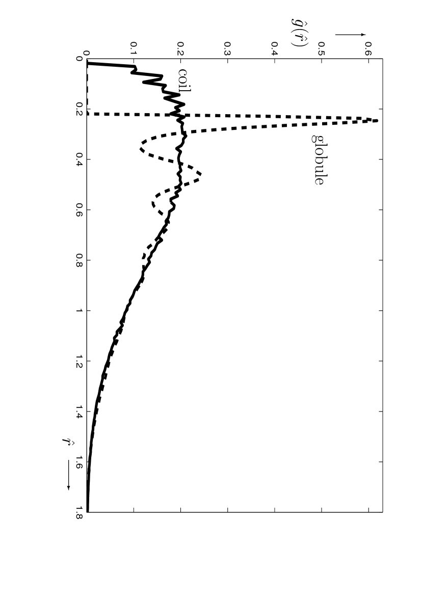
To illustrate the usefulness of our scheme we have investigated the two–point correlation functions of ring, linear and star homopolymers in the coil state, as well as of the globular state of a ring homopolymer since the connectivity is not as important for the latter state. The data for has been obtained by Monte Carlo simulations discussed in our previous study IntraCor . Fig. 2 depicts typical behavior of for an open homopolymer coil and a ring homopolymer globule. As one can see, in the liquid globular state the TPCF has several peaks of increasing width and decreasing height located at approximately (). On the other hand, the TPCF of a coil exhibits a smoother radial dependence, but suffers from a significant statistical noise.
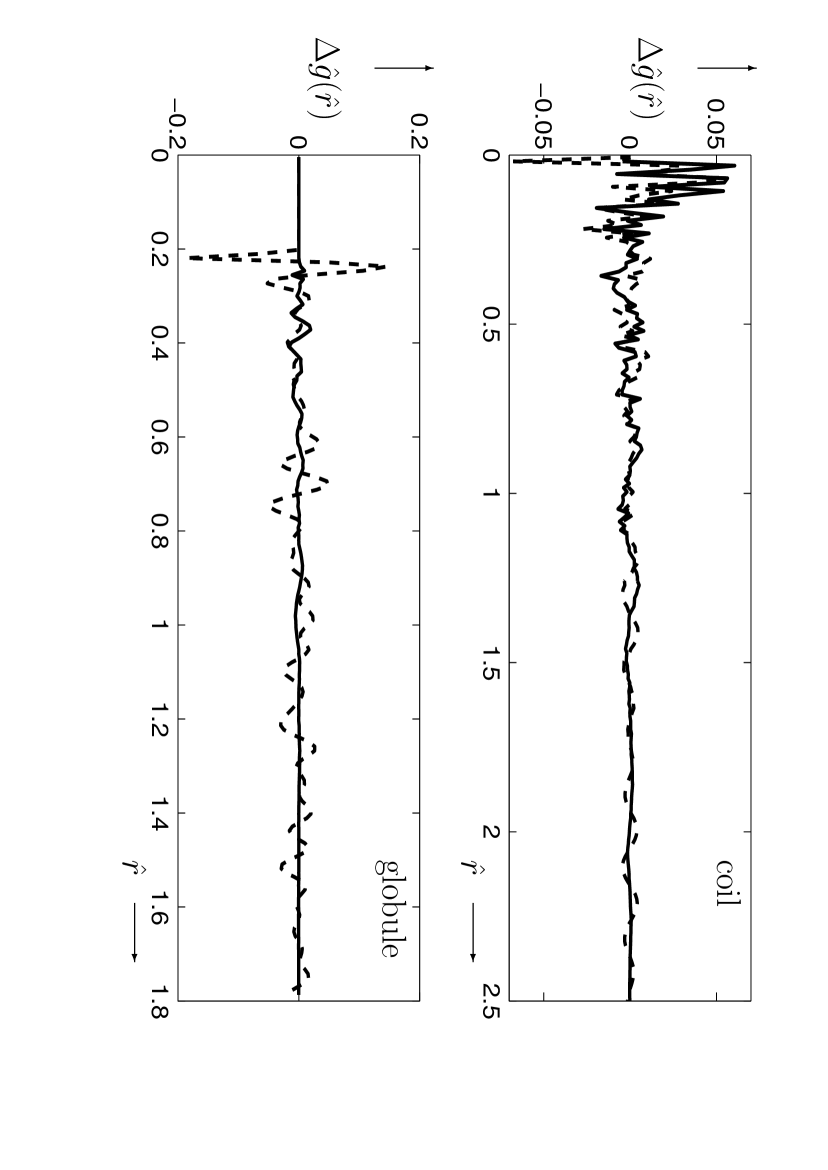
The correlation functions obtained from such data are then approximated by the above described wavelet procedure. Fig. 3 shows the difference of the TPCFs obtained by simulations and their approximations by wavelets (solid curves) and cosines (dashed curves) with the same number of terms . One can clearly see that the wavelet treatment provides a much better approximation than the cosines Fourier treatment. For the coil (), at small radial separations both treatments do show deviations from the simulation data, but these only reflect the limitations of sampling statistics of TPCF as the function should really be very smooth and obey the des Cloizeaux equation. However, while the wavelet treatment gives an essentially vanishing for larger , the Fourier treatment continues to yield parasitic oscillations at all separations. For the globule (), which had a much better quality of data due to a smaller entropy of the globule, the wavelet treatment gives an essentially vanishing everywhere, whereas the Fourier method works very poorly in the whole range with strong oscillations present even for the largest of separations.
In Fig. 4 we present four different levels of the wavelet decomposition of TPCF of an open coil. We can see that the smooth part of this function can be well represented by the approximation coefficients. Conversely, the unpleasant oscillations are concentrated in the detail coefficients.
In Fig. 5 we likewise present four different levels of the wavelet decomposition of TPCF for the globule of a ring homopolymer. We can see that the smooth part of this function can be mainly represented by the approximation coefficients. But there is also an important information in the detail coefficients, which mainly represent the sharp peaks of the function. Therefore, our ‘smart’ level–by–level technique allows us to effectively suppress noise in case of the coil and to prevent us from ‘oversmoothing’ of physical oscillations in case of the globule.
We have also calculated the mean square norm of the inaccuracy , which characterizes the quality of the approximation: , where are the grid points, is the ‘true’ correlation function from Monte Carlo data, and is the approximated one. Figs. 6 and 7 depict the dependences of the norm on the number of the approximating coefficients for the coil and globule states respectively. In what was mentioned above we have used the ‘RB5-5’ basis set daubechies . Here, for comparison we also depict these dependencies for the Cosine and FFT approximation, which are widely used in applications marpl . We can see that for a reasonable number of coefficients the wavelet approximations gives us a remarkably better accuracy than the conventional methods.
For the approximated TPCF we have also evaluated the scaling exponents for the coil state. In this case we can compare these results with the rather accurate theoretical values obtained from the Borel resumed renormalisation group calculations CloizeauxBook ; Schafer ; Guida ; Caracciolo . As in Ref. IntraCor the fitting has been done via the the nonlinear least–squares (NLLS) Marquardt–Levenberg method NumerRecip by means of the fit function in the gnuplot software. Fit reports parameter error estimates which are obtained from the variance–covariance matrix after the final iteration. By convention, these estimates are called ‘standard errors’ and they have been reported in Tab. 1, which contains the results for open and ring homopolymers. Here we have used the wavelet approximation with coefficients. In this table we also include the results which are obtained from the fitting of the untreated functions as in Ref. IntraCor . The notations in the first column follow the des Cloizeaux convention: 0 — end–end monomers, 1 — end–middle, 1’ — end–three quarters, 1” — end–one quarter, and 2 — one quarter–three quarters of the chain respectively. Here and below reported errors are those from the fitting procedure only and do not necessarily account for statistical and other simulation errors.
We can see that the wavelet approximated functions agree with the most recent theoretical values much better. Note also that some of the theoretical values in this table have been updated thanks to the more accurate values from Refs. Schafer ; Guida ; Caracciolo as compared to those which we have used in Ref. IntraCor . Moreover, we do not even need to freeze at the theoretical value in order to extract a more accurate estimate for as we had to do previously. These improvements in the results of our fitting are not surprising given that, as we have mentioned earlier, the coefficients cut–off leads to an effective noise suppressing.
The least–squares fitting of the data with a model function , which depends on the fitting parameters in a nonlinear fashion, in the multi–variate case is a complex problem NumerRecip akin to that of finding the global minimum of the merit function with respect to parameters , where is the standard deviation (error) of the i-th data point. If the data is fairly noisy, the problem of finding the global minimum of becomes complicated as there are many low–lying local minima of this function and its constant value surfaces have a complicated topology. The Marquardt–Levenberg method is one of the most popular fitting algorithms which is an efficient hybrid of the inverse–Hessian (variable metric) and the steepest descent (conjugated gradients) minimization algorithms for NumerRecip . Practically, the iterations need to be stopped after the values of change less than the specified precision and, clearly, the resulting fitted values may depend on the choice of the initial values if there are many local minima present, as well as on the weights . It is not uncommon to find the parameters wandering around near the global minimum in a flat valley of complicated topology if the input data was fairly noisy NumerRecip . The wavelet treatment renders the initial poorly–defined fitting problem into a well–defined one (which becomes essentially independent of the initial parameters choice) by removing the high–pitch statistical noise from the data, and thus by simplifying the topology of the constant surfaces and getting rid of its many artificial local minima. At the same time, the variances (squared standard errors) of the fitted parameters and the co-variances between them become smaller than for the untreated data as we are now guaranteed to have found the true global minimum.
Tab. 2 lists similar exponents for star homopolymers with the number of arms in a good solvent. Here we have used the wavelet approximation with coefficients. We then have compared the results with those from the analytical renormalisation group calculations in the so–called ‘cone’ approximation for from Ref. Ferber . This comparison has not been previously made in Ref. IntraCor or elsewhere so far, to the best of our knowledge. The agreement between the Monte Carlo and theoretical values seems quite reasonable despite the relatively short length of the arms and the limitations of the ‘cone’ approximation. The latter produces the contact exponents only dependent on the functionalities , of the two monomers in question and not on any other parameters of the star, namely
| (18) |
As one can see, the quality of the wavelet approximation is rather good for the combined scheme, while the number of approximating coefficients is quite small.
In general, the accuracy of the wavelet approximations with a fixed number of reconstruction coefficients depends on the chosen basis set. So far, no exact ‘recipe’ was given on which base we have to use in a concrete case. Thus, we have checked our assumption about one of the dual bases ‘RB5-5’ by an additional study. As we are especially interested in the quality of the scaling exponent calculations we have evaluated the scaling exponent for an open homopolymer coil with the use of different bases. These results are presented in Tab. 3. We have used the wavelet approximations of the end–end TPCFs with the same number of coefficients. We chose for this comparison typical representatives of the main wavelet families: Coifman 2, Daubechies 4, Symlet 4, Biorthogonal 5-5 and Discrete Meyer wavelets daubechies .
We can see that the ‘Reverse Biorthogonal 5-5’ basis set does the approximation better than the other bases. On the other hand, other bases, apart from the Discrete Meyer’s, also reveal good fitting results compared to the untreated TPCF. This means that our current scheme is just one of possible successful choices of the basis set. The situation with the Discrete Meyer is easily explained by a too large support length of this basis as compared with for ‘RB5-5’, which is known to lead to strong over–smoothing daubechies .
IV Conclusion
Our present study indicates that the discrete wavelets is a suitable and powerful instrument for approximating the intra–chain two–point correlation functions (TPCF) of different homopolymers in dilute solutions. The wavelet technique allows us to extract the scaling properties from fairly noisy data more accurately and reliably than it can be done by the direct fitting. The wavelet treatment removes the high–pitch stochastic fluctuations (part of ‘statistical noise’) in the data thereby producing a somewhat ‘coarse–grained’ approximation of the data. This renders the ill-defined multi–variate nonlinear fitting procedure of the untreated data into a well–defined uniquely convergent fitting procedure after the wavelet treatment of the data. Naturally, this also reduces the standard deviations of the fitted parameters. However, the wavelet treatment does not over–smooth the data by retaining the genuine oscillations as we clearly see in the case of the globule, nor does it produce any of the unpleasant artefacts of the truncated Fourier approximation.
We can see that the dual basis set performs particularly well for approximating TPCFs. This is related to the basis properties, namely, that the decomposition functions have a maximal number of vanishing moments with a finite support, whereas the reconstruction functions are as regular as possible with a given length of support. Moreover, the proposed scheme is rather flexible as it is based on the conventional FWT algorithm. One can choose the basis set and adjust the number of the coefficients easily for a particular problem. From the results in Tab. 3 we can also conclude that by using almost any reasonable basis it is possible to obtain an improvement in the fitting procedure.
It should be emphasized that the wavelet scheme is rather universal. The scheme of the wavelet approximation proposed here allows us to represent the correlation functions with a small number of approximating coefficients not only for the coil but also for globular state of the homopolymers. For instance, our procedure yields the relative accuracy of the approximation of order . Such accurate knowledge of TPCFs can be used for an input to the self–consistent calculations of the inter–chain distribution functions in the framework of the density functional methods yet98 ; yet03 ; sweat and others.
Due to a compact parameterization and a high accuracy of the approximation by wavelets, we hope that the wavelets can be applied not only for approximating the inter–chain distribution functions of polymers, but also in order to calculate these functions by the integral equations theory of polymers monson . The success of the recent applications of wavelets to the theory of molecular solutes chuevfedorov1 has indicated that the method is capable of calculating the thermodynamic characteristics of solvation rather accurately.
We believe that further progress in this direction can also be of importance for the novel theories for calculating the intra–chain TPCFs of polymers directly from a force field. Some of us are presently working on the Super–Gaussian Self–Consistent (SGSC) theory for a single macromolecule with any two–body Hamiltonian, in which a set of integro–differential equations is derived for as well as for . In order to reduce the computational expenses in such calculations, having a compact and multi–resolution accurate representation for is essential.
Finally, due to the very general nature of the wavelet theory, we hope that wavelets can find other numerous applications for describing spatial and temporal dependences of various observables in a number of fields of soft condensed matter theory which they have not hereto beneficially influenced.
Acknowledgements.
We would like to thank Professor L. Schäfer, Dr C. von Ferber, Dr H.-J. Flad, Dr H. Luo and Professor D. Kolb for interesting discussions. We acknowledge the support of the Centre for Synthesis and Chemical Biology, and some of us (M.F. and G.C.) also acknowledge the support of the Russian Foundation for Basic Research.References
- (1) J. des Cloizeaux, G. Jannink, Polymers in Solution, Oxford Science Publ. (1990) .
- (2) J.-P. Hansen and I. R. McDonald, Theory of Simple Liquids. 2-nd ed., Academic, London (1986).
- (3) L. Schäfer, Excluded volume effects in polymer solutions as explained by the Renormalisation Group, Chapter 16, Springer–Verlag, Berlin (1999); L. Schäfer, U. Lehr, C. Kappeler, J. Phys. I 1, 211 (1991).
- (4) G.N. Chuev, M.V. Fedorov, J. Comput. Chem. 25, 1369, (2004).
- (5) G.N. Chuev, M.V. Fedorov, J. Chem. Phys. 120, 1191 (2004).
- (6) G.N. Chuev, M.V. Fedorov, Phys. Rev. E 68, 027702 (2003).
- (7) S.G. Mallat, A Wavelet Tour of Signal Processing, 2-nd ed., Academic press, San Diego, (1999).
- (8) Y. Meyer, Wavelets: Algorithms and Applications, SIAM, Philadelphia, (1993).
- (9) I. Daubechies, Ten Lectures on Wavelets. CBMS/NSF Series in Applied Math. No. 61, SIAM, Philadelphia, (1992).
- (10) D.L. Donoho, Applied and Computational Harmonic Analysis, 1, pp. 100-115. (1993); D.L. Donoho, M. Vetterli, R.A. DeVore, I. Daubechies, IEEE Trans. Inf. Theory 44, No.6, pp. 2435-2476 (1998).
- (11) R.T. Ogden, Essential Wavelets for Statistical Applications and Data Analysis, Birkhauser, Boston, (1997).
- (12) K. Cho, T.A. Arias, J.D. Joannopoulos, P.K. Lam, Phys. Rev. Lett. 71, 1808 (1993).
- (13) S. Wei, M.Y. Chou, Phys. Rev. Lett. 76, 2650 (1996).
- (14) S. Goedecker, O.V. Ivanov, Comput. Phys. 12, 548 (1998).
- (15) S. Goedecker, Wavelets and Their Application for the Solution of Partial Differential Equations in Physics., Presses Polytechniques et Universitaires Romandes, Lausanne, (1998).
- (16) S. Han, K. Cho, J. Ihm, Phys. Rev. B 60, 1437 (1999).
- (17) S. Goedecker, I. Ivanov, Phys. Rev. B 59, 7270 (1999).
- (18) J.-P. Antoine, Ph. Antoine, B. Piraux, in: Wavelets in Physics, edited by J. C. van den Berg (Cambridge University Press, Cambridge, 1999), p. 299.
- (19) T.A. Arias, Rev. Mod. Phys. 71, 267 (1999).
- (20) H.-J. Flad, W. Hackbusch, D. Kolb, R. Schneider, J. Chem. Phys. 116, 9641 (2002).
- (21) H. Luo, D. Kolb, H.-J. Flad, W. Hackbusch, T. Koprucki, J. Chem. Phys. 117, 3625 (2002).
- (22) A. B. Romeo, C. Horellou, J. Bergh, MNRAS, 342, 337 (2003).
- (23) R. Guida, J. Zinn–Justin, J. Phys. A 31, 8103 (1998).
- (24) E.G. Timoshenko, Yu.A. Kuznetsov, Colloids and Surfaces, A 190, 135 (2001).
- (25) Yu.A. Kuznetsov, E.G. Timoshenko, J. Chem. Phys., 111, 3744 (1999).
- (26) F. Ganazzoli, Yu.A. Kuznetsov, E.G. Timoshenko, Macromol. Theory Simul. 10, 325 (2001).
- (27) M.P. Allen and D.J. Tildesley (Ed.), Computer Simulation of Liquids, Clarendon Press, Oxford, (1987)
- (28) E.G. Timoshenko, Yu.A. Kuznetsov, R. Connoly, J. Chem. Phys. 116, 3905 (2002).
- (29) W. Sweldens, Appl. Comput. Harm. Anal. 3(2), 86 (1996).
- (30) G. Belkyn, R. Coifman, V. Rokhlin, Comm. Pure Appl. Math. 44, 141 (1991).
- (31) S.L. Marpl, Jr., Digital spectral analysis with applications, Prentice-Hall, New Jersey, (1987).
- (32) S. Carraciolo, M.S. Causo, A. Pelisetto, J. Chem. Phys. 112, 7693 (2000).
- (33) C. von Ferber, A. Jusufi, M. Watzlawek, C.N. Likos, H. Löwen, Phys. Rev. E 62, 6949 (2002); C. von Ferber, Nucl. Phys. B 490, 511 (1997).
- (34) W.H. Press, S.A. Teukolsky, W.T. Vetterling, B.P. Flannery, Numerical Recipes in C, Cambridge University Press, (1992).
- (35) A. Yethiraj, J. Chem. Phys. 109, 3269 (1998).
- (36) N. Patra, A. Yethiraj, J. Chem. Phys. 118, 4702 (2003).
- (37) M.B. Sweatman, J. Phys.: Condens. Matter 15, 3875 (2003).
- (38) K.S. Schweizer, J.G. Curro, Integral Equation Theories of the Structure, Thermodynamics and Phase Transitions of Polymer Fluids, in: Adv. in Chem. Phys., 98, 1 (1997); P.A. Monson, G.P. Morriss, Adv. Chem. Phys. 77, 451 (1990).
| 0 | ||||||
| 1 | … | |||||
| 1’ | … | |||||
| 1” | … | |||||
| 2 | … | |||||
| Ring | … |
| 0, a:m=25 | |||||
|---|---|---|---|---|---|
| 0, a:m=50 | |||||
| a:n=25, a:m=50 | |||||
| a:n=50, b:m=50 |
| Theoretical | ||
|---|---|---|
| ‘RB5-5’ | ||
| ‘BR5-5’ | ||
| Daubechies 4 | ||
| Symlet 4 | ||
| Coifman 2 | ||
| Discr. Meyer | ||
| Untreated |
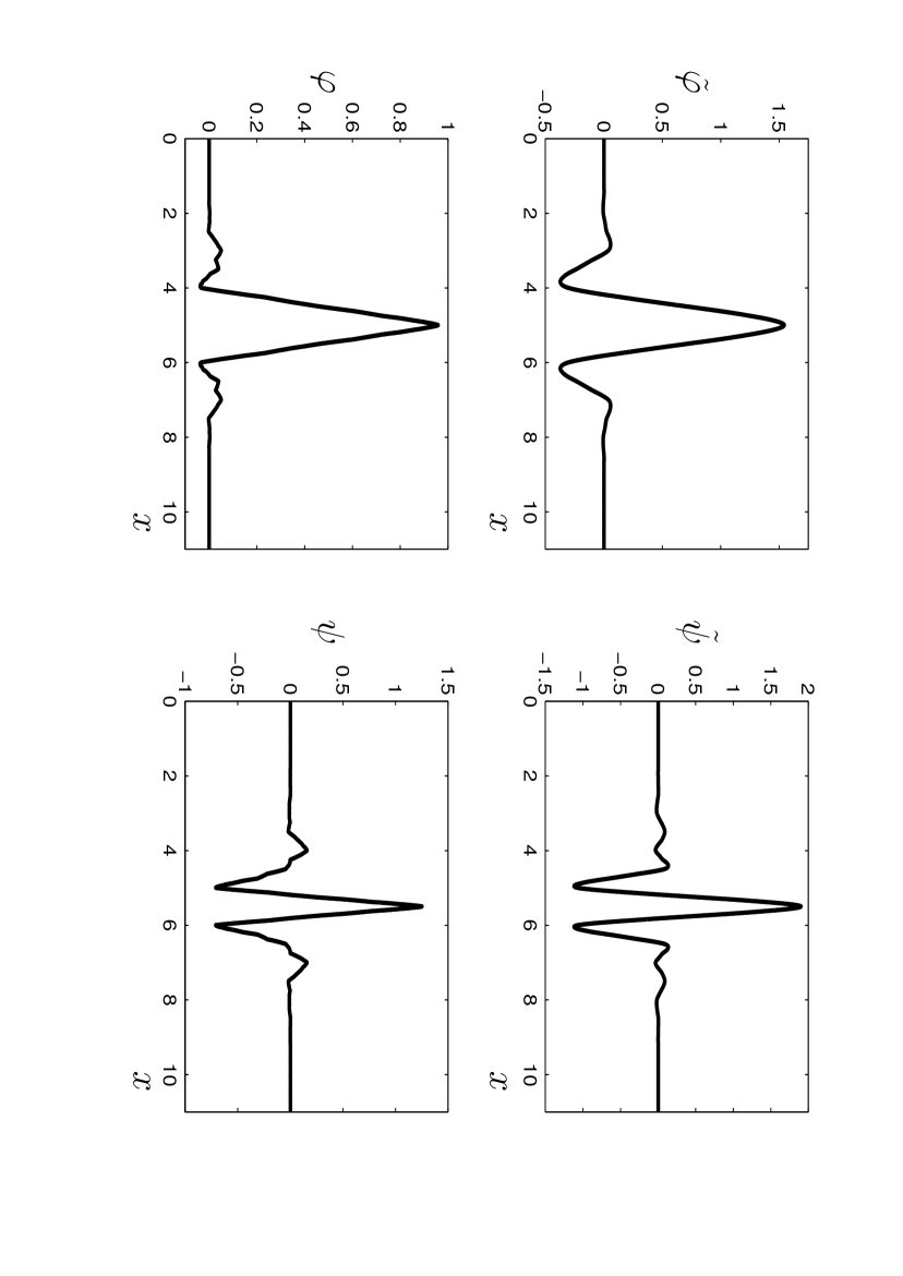
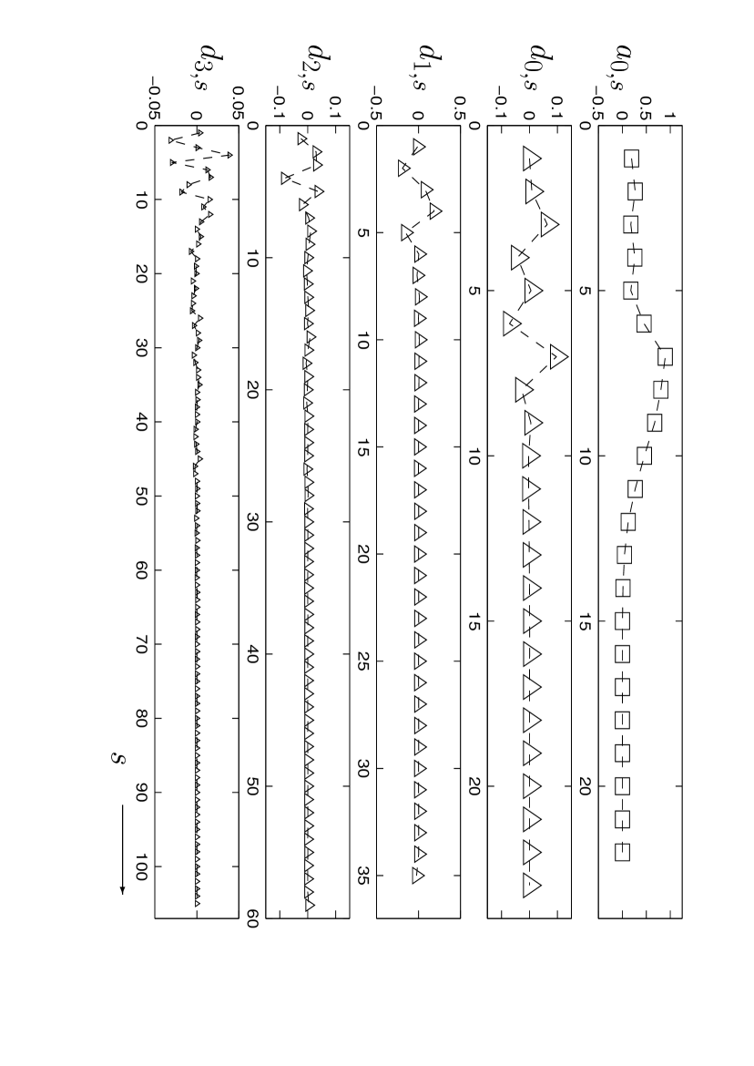
At the top there are approximating coefficients at the level . The detail coefficients are presented in the ascending order in the level of the resolution vs the shift parameter .

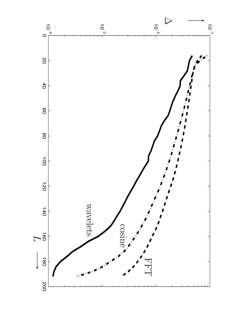
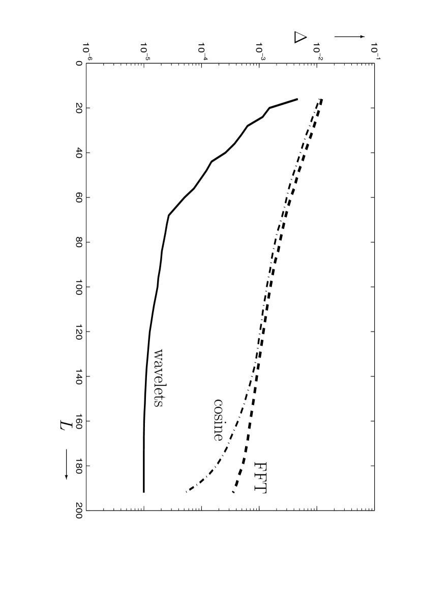
The curves correspond to the wavelet approximation (solid line), FFT approximation (dashed line) and cosine approximation (dash–dotted line). The X-axis is the number of approximation coefficients used.