We consider the nucleation process associated with capillary condensation of a vapor in a hydrophobic cylindrical pore (capillary evaporation). The liquid-vapor transition is described within the framework of a simple lattice model. The phase properties are characterized both at the mean-field level and using Monte-Carlo simulations. The nucleation process for the liquid to vapor transition is then specifically considered. Using umbrella sampling techniques, we show that nucleation occurs through the condensation of an asymmetric vapor bubble at the pore surface. Even for highly confined systems, good agreement is found with macroscopic considerations based on classical nucleation theory. The results are discussed in the context of recent experimental work on the extrusion of water in hydrophobic pores.

PACS:

1 Introduction

Recently, the study of water confined in hydrophobic pores has been the object of a growing interest, both from the fundamental and the industrial point of view [1, 2, 3, 4, 5, 6]. A specific feature of such mesoporous materials is the strong adsorption of the wetting phase occuring at a chemical potential (or pressure) lower than the bulk saturation value. This behavior is usually known as capillary condensation, and corresponds fundamentally to the shifted liquid-gas phase transition induced by confinement [7]. In the case of hydrophobic pores, the wetting phase is the vapor while the non wetting phase is the liquid. The restricted geometry therefore favors nucleation of vapor bubbles inside the pores. This is known as the hydrophobic effect in chemistry, widely study by Chandler and co-workers [8, 9, 10, 11].

A characteristic of capillary condensation (both in hydrophobic and hydrophilic porous matrices) is the existence of a large hysteresis of adsorption. Two different origins have been pointed out to explain this behavior. One is the presence of large energy barriers to nucleate the wetting phase (below its saturation value) [12]. Another explanation, valid in particular for disordered mesoporous matrices, is the trapping of the system in a complex free energy landscape [13, 14]. There is in general an intricate coupling between these two origins of hysteresis. However, limiting cases might be considered experimentally. Highly disordered mesoporous materials (such as porous glasses or silica gels) must be described using the approach of reference [14]. For ”ideal” systems with regular pore shapes, such as MCM-41, a more standard thermodynamic approach is appropriate [15].

In the following we focus on adsorption in such ”ideal” materials. The slit pore geometry, in which fluids are confined between a pair of infinite plate, has first been considered in the literature [3, 16, 17]. A macroscopic approach was used by Restagno et al. to determine free energy barriers [18], which proved to be very large. Talanquer et al. [19] used density functional theory (DFT) to tackle this problem and showed that the macroscopic description yields results in quantitative agreement with DFT provided the effect of line tension is taken into account. Nucleation path proposed along these approaches are in agreement with those determined by molecular simulations using sampling methods [3] developed by D. Chandler’s group [20, 21].

The experimentally relevant case of cylindrical pores has been considered more recently by Kornev and Neimark [22] and Lefevre et al. [15] along the same lines. An important difference with the slit case, however, is that the curvature of the pore may lead to a critical nucleus lacking axial symmetry [15]. The latter results have been compared with experimental data on hydrophobic MCM-41 materials, showing good agreement with the measured hysteresis and estimated nucleation barriers.

In this paper, we investigate nucleation in a hydrophobic cylindrical pore using a lattice functional density approach. Our aim is twofold : (i) assess the pertinence of the macroscopic theory to describe nucleation under strong confinement; (ii) consider the possibility of nucleation paths involving asymmetric nuclei, which we previously predicted on the basis of macroscopic arguments to be energetically favorable [15]. To this end, we consider a very simple coarse grained model, which takes fluid-fluid and fluid-solid interactions into account at the most simple level. Critical temperature and chemical potential at coexistence as well as liquid-vapor interfacial tension and contact angle value are computed using both mean field calculations and Monte Carlo simulations. Umbrella sampling is used to determine nucleation paths, critical nuclei and reduced energy barriers.

2 Model

2.1 Microscopic Hamiltonian : mean-field and fluctuations

Our model is defined by the Hamiltonian proposed by Kierlik et al. to describe a confined inhomogeneous fluid in contact with an external reservoir of temperature T and chemical potential $\mu$ [23, 13, 24] :

$$H({\rho_{i}})=k_{B}T\sum_{i}[\rho_{i}ln\rho_{i}+(\eta_{i}-\rho_{i})ln(\eta_{i}-\rho_{i})]-\mu\sum_{i}\rho_{i}$$ (1)

$${}-w_{ff}\sum_{<ij>}\rho_{i}\rho_{j}-w_{mf}\sum_{<ij>}[\rho_{i}(1-\eta_{j})+(1-\eta_{i})\rho_{j}]$$

In this expression, $1-\eta_{i}$ are the (discrete) occupancy variables for the matrix ($\eta_{i}=0,1$ for the matrix/fluid site) and $\rho_{i}$ is the local density of the fluid on a three-dimensional (BCC) lattice ($\rho_{i}\in[0,1]$). The fluid-fluid $w_{ff}$ and matrix-fluid $w_{mf}$ interactions only act between nearest neighbors sites ($<ij>$) and the ratio $w_{mf}/w_{ff}$ determines the wettability of the matrix. This coarse-grained description leaves aside most of the microscopic details of an actual solid-fluid system but allows extensive simulations while retaining the main experimental and physical ingredients of the system under consideration. In particular it is sufficient to describe, at least qualitatively, the interplay between volume and surface contributions of the free energy (here in a curved, cylinder like, geometry). At this point, one may notice that the above Hamiltonian is equivalent to the coarse-grained version of the well known site-diluted Ising-Model [25].

The cylindrical pore is represented in figure 1, together with the underlying BCC lattice. Periodic boundary conditions are applied in the direction parallel to the axis of the cylinder. The BCC lattice representation of a cylinder might appear crude, but, as already mentioned above, this proves sufficient to study the generic mechanism of nucleation in a curved geometry.

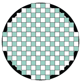
Figure 1: Representation of the section of a cylindrical pore in the BCC lattice model. The sites shown belong to the fluid ($\eta_{i}=1$). The main axis of the cylinder is along a (100) direction the cubic lattice. The radius of the cylinder is here 5.5 lattice spacings.

We have investigated the phase properties of the above Hamiltonian in equation 1, at two levels of description. First at the mean field level, where the previous Hamiltonian is identified as the free energy of the system; second, by performing finite temperature Monte Carlo simulation of the Hamiltonian (equation 1) in order to incorporate fluctuation effects.

Before turning to the nucleation properties, we briefly characterize the bulk and surface properties of the system.

2.2 Bulk Phase properties

In the bulk, the system undergoes a liquid-vapor phase transition. At the mean field level, this is easily deduced from the equation of state which is found to take the form

$$\mu=k_{B}T\ln\frac{\rho_{bulk}}{1-\rho_{bulk}}-zw_{ff}\rho_{bulk}$$ (2)

where $\rho_{bulk}$ is the uniform density of the bulk fluid and $z=8$ is the lattice coordination number. The mean-field bulk liquid-gas transition is then found to take place at $\mu_{sat}/w_{ff}=-4.0$, with a critical point located at $k_{B}T_{c}/w_{ff}=2.0$. The resulting mean-field bulk phase diagram is plotted in figure 2.

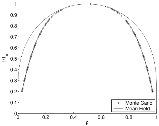
Figure 2: Bulk phase diagram, obtained from mean field (full curve) and Monte-Carlo (dots) approaches.

Beyond mean field, fluctuations are incorporated by performing Monte Carlo simulations based on the Hamiltonian in equation 1. A few technical comments are in order here. The standard Metropolis method is used [25, 26], in the grand canonical ensemble (which amounts here to simply fixing the chemical potential $\mu$ of the fluid). One Monte Carlo step corresponds to one attempted trial move per fluid lattice site. The density change in the trial moves is $0.2$, corresponding to a typical acceptance rate of $0.5$.

The bulk phase diagram is computed using periodic boundary conditions, with a cubic simulation cell of size $L$. The liquid-vapor equilibrium is determined by equality of the grand potential in the two phases. The latter is computed by thermodynamical integration of

$$\frac{\partial\Omega}{\partial\mu}=-<\rho>$$ (3)

with boundary conditions

$$\lim_{\mu\to-\infty}\Omega_{v} = 0$$ (4)

$$\lim_{\mu\to+\infty}\Omega_{l} = -(\mu+4w_{ff})$$ (5)

The simulated phase diagram is plotted in figure 2 (for a lattice size $L=15$, corresponding to $2\times 15^{3}$ sites of the underlying BCC lattice). The value $\mu_{sat}/w_{ff}=-4.0$ gives a very good approximation of the chemical potential on the critical line, (independently of the temperature $T$). The critical temperature is found to be $k_{B}T_{c}/w_{ff}\simeq 0.5$, quite smaller than the mean-field result ($k_{B}T_{c}/w_{ff}=2$). If fluctuations are expected to decrease the critical temperature in spin-Ising model, such a large difference is however surprising and seems to be due to the coarse graining of the order parameter $\rho$.

2.3 Surface properties

In this section, we compute numerically the liquid vapor surface tension and the contact angle of the triple line on the solid surface. These ingredients will be needed to check the accuracy of the macroscopic calculation used to describe the nucleation problem in section 3.

2.3.1 Liquid-Vapor surface tension

Generally, the liquid vapor surface tension is computed by first constructing a liquid- vapor interface and then computing the excess free energy (grand potential) of this interface compared to the bulk coexistence free energy. However in a lattice model, the surface free energy does depend on the particular direction of the interface with respect to the underlying lattice axis.

This dependence is emphasized below using the simple mean field approach. In the presence of an interface, minimization of the (mean-field) Hamiltonian (1) with respect to the local fluid densities, yields a set of non linear coupled equations

$$\rho_{i}=\frac{\eta_{i}}{1+e^{-\beta\{\mu+\sum_{j/i}[w_{ff}\rho_{j}+w_{mf}(1-\eta_{j})]\}}},$$ (6)

where the sum is over the nearest neighbors $j$ of site $i$. We have solved numerically these equations by simple iterations $\{\rho_{i}^{t+1}\}=f(\{\rho_{i}^{t}\})$ starting from an initial distribution $\{\rho_{i}^{0}\}$ (with a convergence requirement $\max_{i}|\rho_{i}^{t+1}-\rho_{i}^{t}|<10^{-10}$) with a sharp interface in the desired orientation. Convergence is quite fast due to the relative simple geometries considered here. Once the interfacial profile is constructed, the mean field Grand Potential $\Omega$ is simply computed by the value of the Hamiltonian computed at the saddle point density. The surface tension is then defined as the excess value, computed from the difference between this value and the bulk coexistence grand potential. We plot on figure 3 the temperature dependence of $\gamma_{LV}$ for two specific directions of the interface, along the [100] and [110] planes. We also compare on this figure the value of the surface tension obtained using a mechanical route, based on the dilation of the sample volume, as described in the Appendix. Note the difference between the thermodynamic and mechanical routes in the present case, which can be ascribed here to the underlying mean-field approximation [27]. Moreover another drawback of the mechanical estimate is that it is restricted to the [110] interface, due to lattice effects.

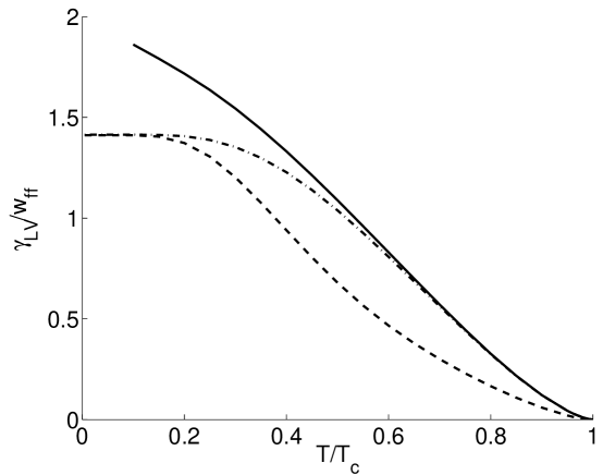
Figure 3: Mean field estimate of Liquid-Vapor surface tension along various directions, as a function of $T/T_{c}$. Solid line: surface tension in the [100] direction, from the excess grand potential. Dash-dotted line: same estimate, now for the [110] interface. Dashed line: estimate from the mechanical route for the [110] interface.

This dependence on the lattice direction remains when fluctuations are included, beyond the mean field approximation. Note however that in contrast to the mean field case, the liquid-vapor surface tension cannot be estimated from the excess grand potential, which is not directly available in the simulation. We have therefore first used the mechanical route, as described in the appendix, to obtain the surface tension from the Monte-Carlo runs.

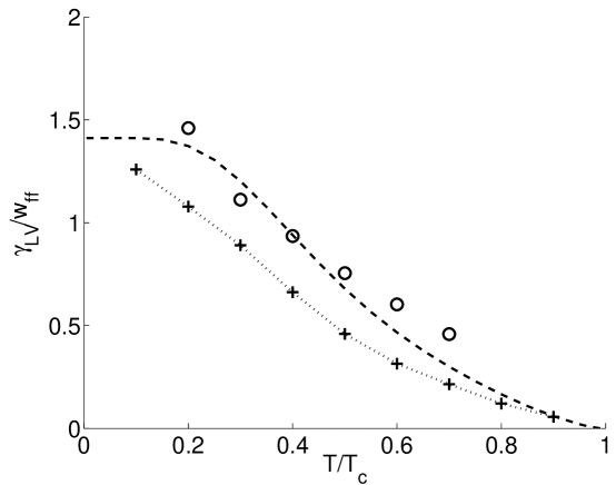
Figure 4: Monte Carlo estimate of liquid-vapor surface tension as a function of $T/T_{c}$. Dotted line with crosses: mechanical estimate (implemented in the Monte Carlo sampling) in the [110] direction. Circles: estimate from the free energy calculation of a liquid bubble (see text for details). Dashed line: mean field calculation for the [110] interface.

A third route can be proposed to estimate the liquid-vapor free energy. Indeed the surface tension can be defined in terms of the free energy necessary to create a bubble of vapor inside the liquid, at coexistence. Moreover this estimate, which results implicitly from an underlying average over the various direction of the lattice grid, is particularly relevant when dealing with the free energy of a nucleated bubble, which will be needed in the next section.

The calculation of the free energy however requires a thermodynamic integration. This is performed using the umbrella sampling technique [20, 26]. At a given temperature, the bulk (periodic) system is placed at the coexistence conditions, obtained from the previous section. An order parameter $\Psi$ is then defined as the number of vapor sites in the system ( with density less than $0.5$). We then constrain the system to contain an average number of vapor sites by biasing the bare Hamiltonian (1). From the technical point of view this is performed by adding a term in $\frac{1}{2}\kappa(\Psi-\Psi_{0})^{2}$ where $\Psi_{0}$ is the target value for sampling. Typical values of $\kappa$ are $0.005$. The Grand Potential curves is then deduced as a function of $\Psi$ by computing the state probability distribution $P(\Psi)$ [26] :

$$\Omega(\Psi)=-k_{B}T\ln\left[P(\Psi)\exp\left({\frac{1}{2}\frac{\kappa(\Psi-\Psi_{0})^{2}}{k_{B}T}}\right)\right]$$ (7)

A matching procedure for the free energy is required as $\Psi_{0}$ is increased from $\Psi_{0}=0$ (liquid state) to $\Psi_{0}\neq 0$ (vapor bubble). For a given order parameter, it can be checked by inspecting the configurations that the vapor sites organize into a vapor bubble with fixed radius $R$. It is then possible to estimate the surface tension $\gamma_{LV}$ from the definition $\Delta\Omega=4\pi\gamma_{LV}R^{2}$.

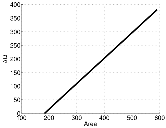
Figure 5: Umbrella sampling estimate of the liquid vapor $\gamma_{LV}$. The measured grand potential is plotted as a function of the liquid-vapor area. Numerical parameters are $T/T_{c}=0.4$ and $\mu/w_{ff}=-4.0$ (corresponding to the liquid-vapor coexistence). The stiffness $\kappa$ of the biasing potential is $\kappa=0.01$ and the total system size is $2\times 20^{3}$ sites.

As shown in figure 5, the measured grand potential exhibits a linear slope as function of the liquid-vapor area, as expected. This allows to define unambiguously the liquid-vapor surface tension. The latter is ”averaged” over the various directions of the underlying lattice grid. This ”spherical” estimate of the liquid-vapor free energy is compared in figure 4 with the value of the surface free energy along the [110] direction.

2.3.2 Contact Angle

The contact angle is another necessary ingredient in the classical description of nucleation phenomena on surfaces [28]. It is defined in terms of the various surface free energies, liquid-vapor (LV), solid-liquid (SL) and solid-vapor (SV), according to Young’s law, $\cos(\theta)=\frac{\gamma_{SV}-\gamma_{SL}}{\gamma_{LV}}$. This requires the computation of the solid-liquid and solid-vapor surface free energies. As for the case of the liquid-vapor surface free energy, these quantities depend on the specific orientation of the interface with respect to the underlying lattice. Technically, planar liquid-solid or vapor-solid interfaces are constructed and the surface free energies are computed along the same lines as for the liquid-vapor surface tension (both in the mean-field and Monte-Carlo calculations).

The mean field results are displayed in figure 6. The comparison between the contact angle computed for various directions of the underlying lattice shows only a weak dependence of the contact angle on the direction of the interface.

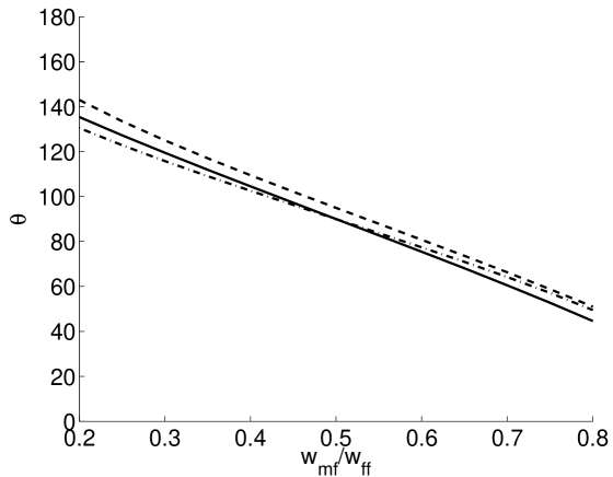
Figure 6: Mean field estimate of contact angle along various directions at $T/T_{c}=0.4$ as a function of $w_{mf}/w_{ff}$. The symbols are the same as in figure 3.

Beyond mean-field, the previous method based on a biased Hamiltonian can be used. A liquid bubble is created on a planar solid surface by adding to the Hamiltonian a penalty associated with the number of liquid sites (see figure 7).

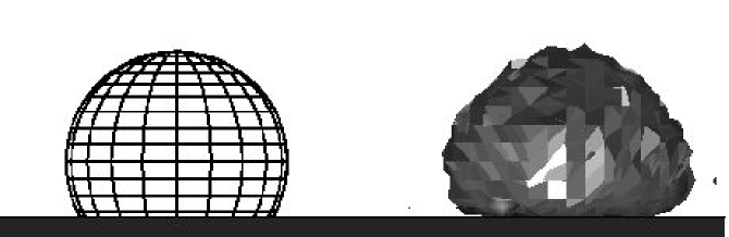
Figure 7: Snapshot of a liquid drop growing on a planar surface in direction [100] ($w_{mf}/w_{ff}=0.3$, $T/T_{c}=0.4$, $1500$ liquid sites) compared with a macroscopic drop with a $120^{\circ}$ contact angle. $\kappa=0.02$. One can check that the underlying BCC lattice does not affect the spherical shape of the bubble.

The free energy is computed accordingly from the matching of the histograms, as in equation (7). The contact angle is computed by comparing the measured free energy with the prediction of macroscopic theory. The latter predicts that the excess grand potential is proportional to the $V^{2/3}$, where $V$ is the volume of the drop:

$$\Delta\Omega=4\pi\gamma_{LV}g(\theta)^{1/3}(\frac{3}{4\pi}V)^{2/3}$$ (8)

Knowing $\gamma_{LV}$ from the spherical estimate in the previous section, the slope of the curve (see figure 8) can be used to extract the contact angle, using $g(\theta)=(2+3\cos(\pi-\theta)-\cos(\pi-\theta)^{3})/4$. This estimate remains however direction dependent, since no averaging over the orientations of the solid is involved. Two calculations for interfaces in the directions [100] and [110] were performed.

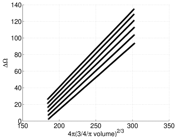
Figure 8: Umbrella sampling estimate of the contact angle $\theta$ for a plane normal to direction [100] as a function of the wettability $w_{mf}/w_{ff}$ at $T/T_{c}=0.4$. $\gamma_{LV}=0.93515$. From top to bottom $w_{mf}/w_{ff}=0.20,\leavevmode\nobreak\ 0.25,\leavevmode\nobreak\ 0.30,\leavevmode\nobreak\ 0.35,\leavevmode\nobreak\ 0.40,\leavevmode\nobreak\ 0.45$. The measured grand potential of a bubble on a planar surface is plotted as a function of the power 2/3 of the volume. $\mu/w_{ff}=-4.0$, $\kappa=0.01$.

As for the mean-field case, the resulting contact angle is found to be only weakly dependent on the direction of the interface. This is shown in figure 9 where the different estimates are compared. The small difference between the two orientations is likely due to a change in the solid coordination number for a liquid site near the interface (4 in [100] direction, 2 in [110] direction).

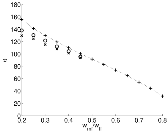
Figure 9: Monte Carlo estimate of contact angle along various directions at $T/T_{c}=0.4$ as a function of $w_{mf}/w_{ff}$. The dotted line corresponds to the mechanical estimate (implemented in the Monte Carlo sampling) in the [110] direction. Thermodynamic integration estimates are shown for a [100] (circles) and [110] (crosses) interface.

It is interesting to remark that the contact angles obtained using the umbrella sampling approach for a droplet are slightly smaller than those obtained using the mechanical route, which only involves planar interfaces. This points towards the role of a nonzero line tension, which has been neglected in the analysis of the results shown in figure 8, but will prove important for the critical nuclei described in the next section, in which the length of the three phase line is important.

3 Nucleation Path

We now focus on the nucleation path for capillary desorption. To this end, we use the previously described umbrella sampling technique for a ”biased” system [26]. An order parameter $\Psi$ is defined as the number of vapor sites (with density less than $0.5$) and the Hamiltonian is biased by adding a term in $\frac{1}{2}\kappa(\Psi-\Psi_{0})^{2}$ where $\Psi_{0}$ is the target value for sampling. Typical values of $\kappa$ are $0.005$. State probability distributions $P(\Psi)$ are obtained over a window of range $\Delta\Psi=30$ (see figure 10).

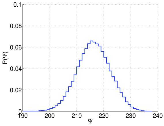
Figure 10: State probability distribution as a function of $\Psi$ obtained for a cylindrical pore of radius $5.5$ and length $30$ at $\mu=-4.0$, $T/T_{c}=0.4$ and $w_{mf}/w_{ff}=0.3$. $\Psi_{0}=230$, $\kappa=0.005$. The distribution is obtained from 2000 monte carlo steps, after 1000 steps of averaging. The difference between the maximum in the probability and the ”imposed” $\Psi_{0}$ is typical of an unstable situation.

The nucleation path is sampled by starting with a filled pore ($\Psi_{0}=0$) and progressively increasing the number of empty sites. For each value of the order parameter, $1000$ Monte Carlo steps where used for equilibration and $2000$ steps for statistics. The final configuration serves as initial configuration for the next order parameter value. Grand potential curves are estimated from the order parameter histogram, using equation (7). As usual, a matching procedure between different order parameter windows is used to obtain the free energy curve. The results are shown in figure 11 for different values of the chemical potential for a cylindrical pore of radius $5.5$ and length $30$.

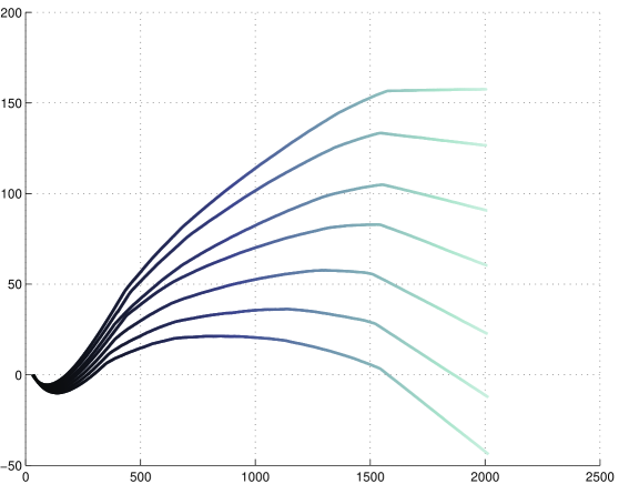
Figure 11: Grand potential as a function of $\Psi$ for a cylindrical pore of radius $5.5$ and length $30$. From top to bottom,$\mu=-3.88$, $\mu=-3.90$, $\mu=-3.92$, $\mu=-3.94$, $\mu=-3.96$, $\mu=-3.98$, and $\mu=-4.0$. $\kappa=0.01$. The sampling windows for $\Psi$ are shifted by 10 units. The final state corresponds to a partially filled pore containing two liquid-vapor interfaces.

A metastability limit of the liquid filled pore is reached around $\Psi=1550$. Once the vapor bubble fills the whole cylinder radius, it adopts a ”cylinder like” shape, whose length increases linearly with $\Psi$. The nucleation barrier is defined as the difference between maximum grand potential and its value in the liquid metastable state. $\Psi=100$ (depending on the chemical potentiel), and corresponds to the presence of a local vapor region near the hydrophobic wall. Such regions are subcritical vapor bubbles that can lead to nucleation. Increasing the order parameter $\Psi_{0}$, a vapor bubble grows in contact with the wall and suddenly turns into a vapor cylinder terminated by two spherical caps.

This approach also yields the shape of the critical nucleus. A typical example is shown on figures 12,13. This shows that the nucleation process occurs via the creation of a vapor bubble on the wall. It is important to emphasize that the nucleus breaks the cylindrical symmetry of the system, in contrast to simple expectations [15].

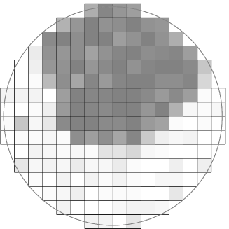
Figure 12: Cross section of a typical umbrella sampling snapshot, before the energy barrier is crossed, for a cylindrical pore of radius $5.5$ and length $30$. The cross section is taken in the plane of symmetry of the bubble. An iso-density surface is represented for $\mu=-3.94$, $\Psi_{0}=1535$.

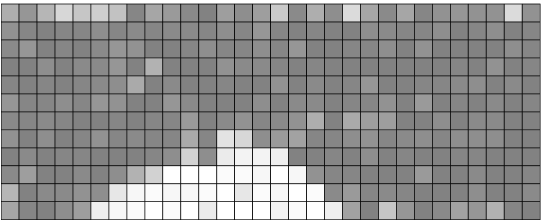
Figure 13: Same as in figure 12, but perpendicular to the axis of the cylinder. Again the cross section is taken in the plane of symmetry of the bubble. Note that both views are representations of the same nucleus, which makes evident the saddle shape of the critical nucleus.

4 Nucleation Barrier

We now gather the results for the energy barrier measured in the simulations, as a function of the various thermodynamic parameters. The temperature of the system is $T/T_{c}=0.4$ giving an averaged liquid-vapor surface tension $\gamma_{LV}=0.93515$ from the thermodynamic integration estimate. The wettability of the confining pore is $w_{mf}/w_{ff}=0.3$. The contact angle is estimated to be $121.7^{\circ}$ in [100] direction and $115.3^{\circ}$ for the [110] interface (see section 2.3.1).

We plot in figure 14 the results for the reduced nucleation barrier $\Delta\Omega/\gamma_{LV}R^{2}$, $R$ being the pore radius. The nucleation barrier is plotted against the ”metastability ratio” $(\mu-\mu_{sat})/(\mu_{eq}-\mu_{sat})$, where $\mu$ is the actual chemical potential, $\mu_{sat}$ is the bulk coexistence chemical potential, and $\mu_{eq}$ is the equilibrium chemical potential for the capillary evaporation in the considered pore of radius $R$. The latter is computed independently, by preparing a configuration in which vapor and liquid phases, separated by a meniscus, are coexisting inside the pore.

From a macroscopic point of view, the excess grand potential between a pore filled of liquid and a pore containing a vapor nucleus can be expressed as

$$\Delta\Omega=V_{V}(P_{L}-P_{V})+\gamma_{LV}A_{LV}+(\gamma_{SV}-\gamma_{SL})A_{SV}$$ (9)

Here $V$ is the volume of vapor phase and $A_{SL}$, $A_{SV}$, $A_{LV}$ are the solid-liquid, solid-vapor and liquid-vapor surface areas. Using reduced quantities $\tilde{V}_{V}=\frac{V_{V}}{R^{3}}$, $\tilde{A}_{LV}=\frac{A_{LV}}{R^{2}}$, $\tilde{A}_{SV}=\frac{A_{SV}}{R^{2}}$, the definition of the contact angle $\cos(\theta)=\frac{\gamma_{SV}-\gamma_{SL}}{\gamma_{LV}}$, and introducing Kelvin’s radius $R_{K}=\frac{\gamma_{LV}}{P_{L}-P_{V}}$, one obtains

$$\frac{\Delta\Omega}{\gamma_{LV}R^{2}}\leavevmode\nobreak\ =\leavevmode\nobreak\ \frac{R}{R_{K}}\leavevmode\nobreak\ \tilde{V}\leavevmode\nobreak\ +\leavevmode\nobreak\ \tilde{A}_{LV}\leavevmode\nobreak\ -\leavevmode\nobreak\ \cos(\pi-\theta)\leavevmode\nobreak\ \tilde{A}_{SV}$$ (10)

The parameter $R/R_{K}$ can be related to the metastability ratio using

$$\frac{\mu-\mu_{sat}}{\mu_{eq}-\mu_{sat}}=\frac{P_{L}-P_{sat}}{P_{L}^{eq}-P_{sat}}\simeq\frac{R}{2R_{K}|\cos(\theta)|}$$ (11)

On the other hand, the reduced areas and volumes, $\tilde{A}_{LV}$, $\tilde{A}_{SV}$ and $\tilde{V}_{V}$, do depend on the specific geometry and morphology of the critical nucleus. In a previous paper, ref. [15], we have proposed a detailed calculation of these quantities and obtained the corresponding energy barrier for a nucleus with an asymetric shape, as observed in the present simulations (see figures 12 and 13). We refer to this paper for further details on these calculations. We only quote a simple and convenient approximation for the energy barrier, which writes

$$\Delta\Omega\leavevmode\nobreak\ =\leavevmode\nobreak\ (P_{L}-P_{V})K_{1}R^{3}+\gamma_{LV}K_{2}R^{2}$$ (12)

with the constants $K_{1}=4.18$ and $K_{2}=2.12$ for $\theta=120^{\circ}$ [15].

Figure 14 shows a comparison between the macroscopic estimate of the nucleation barrier, computed from classical capillarity as described in [15], with results obtained from Monte Carlo simulations for cylindrical pores of radius $R=3.5$, $R=4$, $R=4.5$, $R=5$ and $R=5.5$. The classical capillarity estimate for the reduced barrier does not depend on pore size, as is obvious from dimensional arguments.

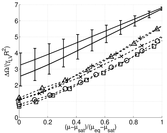
Figure 14: Reduced energy barrier for cylindrical pores of radius $R=3.5$ (circle), $R=4$ (square), $R=4.5$ (cross), $R=5$ (triangle), $R=5.5$ (plus) compared to macroscopic results for a vapor bubble using a $120^{\circ}$ (lower full line) and $115^{\circ}$ (upper full line) contact angle. The error bars corresponds to the same macroscopic estimates, with contact angle between $110^{\circ}$ and $125^{\circ}$. Dotted lines are guides to the eye.

Even allowing for some flexibility in the value of the contact angle, it is clear that that the macroscopic approach overestimates the nucleation barrier, and that the reduced energy barrier obtained from simulation depends on the size of the pore. The good agreement in the slopes suggests however that this discrepancy can be corrected by a simple shift of the classical capillarity estimate of the activation energy, which should depend on pore size and be independent of the chemical potential. As already proposed by Lefevre et al. [15], such a shift can be obtained by invoking the role of line tension, which adds to the nucleation barrier a term proportional to the length of the three phase line in the critical nucleus. Such a line term writes $\tau^{*}\tilde{L}_{SLV}/(\gamma_{LV}R)$, where $\tilde{L}_{SLV}$ is the length of the three phase line.

Such a term is easily taken into account in the previous macroscopic description, as described in ref. [15]. The results, displayed in figure 15, show that a value of the line tension $\tau^{*}/w_{ff}=-0.55/b$ ($b$ being the unit length of the lattice) allows to obtain a very good agreement between the measured free energy barriers and the macroscopic estimate. Again we quote the corresponding convenient approximation of the free energy barrier with the line tension term included (see Eq. (12)):

$$\Delta\Omega\leavevmode\nobreak\ =\leavevmode\nobreak\ (P_{L}-P_{V})K_{1}R^{3}+\gamma_{LV}K_{2}R^{2}+\lambda K_{3}R$$ (13)

with $K_{3}=12.43$ for $\theta=120^{\circ}$ [15].

A few comments are in order. First the negative sign of the line tension is in agreement with previous observations [19, 15]. Moreover, the order of magnitude is consistent with these previous estimates. Indeed, using a typical microscopic length $b\simeq 1$ nm and the value of the critical temperature of water, $T_{c}\simeq 675^{\circ}$ K, we obtain $\tau\leavevmode\nobreak\ \sim 10^{-11}\leavevmode\nobreak\ J/m$ in good agreement with experimental datas.

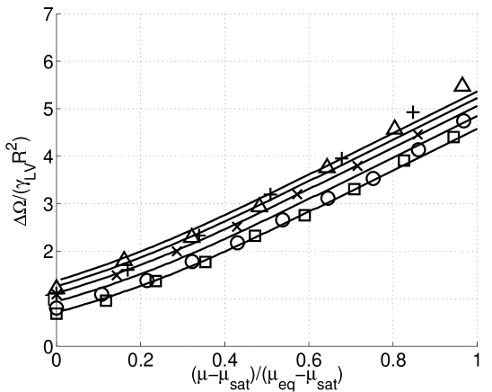
Figure 15: Macroscopic reduced energy barriers for cylindrical pores using a $120^{\circ}$ contact angle and a line tension $\tau^{*}=-0.55w_{ff}/b$ (full lines) compared with Monte Carlo simulations. From bottom to top $R=3.5$, $R=4$, $R=4.5$, $R=5$ and $R=5.5$. The symbols are the same as in figure 14.

5 Conclusion

In this paper a careful estimate of the nucleation barriers for capillary evaporation inside an hydrophobic pore has been proposed. Monte Carlo simulations have shown that capillary evaporation occurs via the nucleation of a vapor bubble at the wall of the cylinder pore. Therefore the critical nucleus does not exhibit the cylindrical symmetry of the cylinder. We have shown moreover that a macroscopic estimate of the free energy is consistent with the measured free energy barriers in a hydrophobic cylindrical pore, provided a contribution from the line tension is included. This conclusion is consistent previous studies [19, 15], and should motivate more direct determination of line tensions in such systems, using experimental or numerical tools.

Annexe A Mechanical calculation of interfacial tension

Consider a $3D$ system of volume $V$ in contact with an external reservoir of temperature T and chemical potential $\mu$ and described by the Hamiltonian ${\mathcal{H}}_{0}$ and partition function $\Theta_{0}$ The system is assumed to contain a liquid-vapor interface of area $A$ normal to the z axis. By transformation $x\to(1+\lambda)x$, $y\to(1+\lambda)y$ and $z\to(1-2\lambda)z$, $dV={\mathcal{O}}(\lambda^{2})$ and $dA=2\lambda A$. the Hamiltonian becomes, to first order in $\lambda$,

$${\mathcal{H}}={\mathcal{H}}_{0}+2\lambda{\mathcal{H}}_{1}$$ (14)

From linear response, the new partition function is given by

$$\Theta=\Theta_{0}+\delta\Theta=\int\exp{-\beta({\mathcal{H}}_{0}+2\lambda{\mathcal{H}}_{1})}\,d\Gamma\approx\int\exp{-\beta{\mathcal{H}}_{0}}(1-2\beta\lambda{\mathcal{H}}_{1})\,d\Gamma$$ (15)

Thus

$$\delta\Theta=-2\beta\lambda<{\mathcal{H}}_{1}>\Theta_{0}$$ (16)

The change $d\Omega$ in the grand potential can be calculated using the macroscopic definition $d\Omega=\gamma dA=2\lambda\gamma A$ or the microscopic approach $\Omega=-k_{B}Tlog\Theta\leavevmode\nobreak\ \Rightarrow\leavevmode\nobreak\ d\Omega=-k_{B}T\delta\Theta/\Theta=2\lambda<\mathcal{H}_{1}>$ leading to the mechanical expression of the interfacial tension :

$$\gamma A=<{\mathcal{H}}_{1}>$$ (17)

Dealing with the Hamiltonian introduced in section 2 on a BCC lattice with cubic axes $\vec{x},\vec{y},\vec{z}$, we write the rescaling of a system with an interface in the plane $(\vec{u}=(1,1,0),\vec{z})$ normal to $\vec{v}=(-1,1,0)$ as $\vec{u}\to(1+\lambda)\vec{u}$, $\vec{z}\to(1+\lambda)\vec{z}$ and$\vec{v}\to(1-2\lambda)\vec{v}$. This is taken into account in the Hamiltonian by assuming a dependence of $w_{ff}$ and $w_{mf}$ as the inverse square length between nearest neighbors sites [18, 27]. Thus ${\mathcal{H}}_{1}$ is obtained as :

$${\mathcal{H}}_{1} =\sum_{<ij>_{(\vec{u},\vec{z})}}w_{ff}\rho_{i}\rho_{j}+w_{mf}[\rho_{i}(1-\eta_{j})+(1-\eta_{i})\rho_{j}]$$ (18)

$$-\sum_{<ij>_{(\vec{v},\vec{z})}}w_{ff}\rho_{i}\rho_{j}+w_{mf}[\rho_{i}(1-\eta_{j})+(1-\eta_{i})\rho_{j}]$$

where $<ij>_{(\vec{u},\vec{z})}$ (resp $<ij>_{(\vec{v},\vec{z})}$) are interaction in the $(\vec{u},\vec{z})$ (resp $(\vec{v},\vec{z})$) plane.

- [1] Maibaum L., Chandler D., J. Phys. Chem. B, 107, 1189 (2003).
- [2] Hummer G., Rasaiah J.C., Noworyta J.P. , Nature, 414, 188 (2001).
- [3] Bolhuis P.G., Chandler D. , J. Chem. Phys., 113, 8154 (2000).
- [4] Barrat J-L., Bocquet L., Phys. Rev. Lett., 82, 4671 (1999).
- [5] Eroshenko V.A. ,Regis R.C., Soulard M., Patarin J., J. Am. Chem. Soc., 123, 8129 (2001).
- [6] Martin T., Lefevre B. et al, Chem. Commun., 1, 24 (2002).
- [7] Gelb L.D., Gubbins K.E., Radhakrishnan R., Sliwinska-Bartkowiak M., Rep. Prog. Phys., 62, 1573 (1999).
- [8] Chandler, D. Nature, 417, 491 (2002)
- [9] Maibaum, L., A. R. Dinner and D. Chandler. J. Phys. Chem. B (In Press)(2004).
- [10] TenWolde P. R, D. Chandler D., Proc. Nat. Ac. Sci.,99, 6539-6543 (2002).
- [11] Huang, D.M, Chandler D., J. Phys. Chem. B, 106, 2047-2053 (2002).
- [12] Huang, D. M. and D. Chandler, Phys. Rev. E 61, 1501-1506 (2000).
- [13] Kierlik E. , Monson P.A., Rosinberg M.L., Tarjus G., J. Phys.: Condens. Matter, 14, 9295 (2002).
- [14] Rosinberg M.L., Kierlik E., Tarjus G., Europhys. Lett. 62, 377 (2003)
- [15] Lefevre B., Saugey A., Barrat J-L. Bocquet L., Charlaix E., Vigier G., Gobin. P-F., J. Chem. Phys. 120, 4927-4938 (2004)
- [16] Lum K., Chandler D., Int. J. Thermo.,19, 845-855 (1998).
- [17] K. Lum A. Luzar, Phys. Rev. E, 56, 6283 (1997).
- [18] Restagno F., Bocquet L., Biben T., Phys. Rev. Lett., 84, 2433 (2000).
- [19] Talanquer V., Oxtoby D.W., J. Chem. Phys., 114, 2793 (2001).
- [20] Bolhuis, P. G., Chandler D., Dellago C., Geissler P., Ann. Rev. of Phys. Chem.,59, 291-318 (2002).
- [21] Dellago, C. and D. Chandler, Lect. Notes in Phys., 605, 321-333(2002).
- [22] Kornev K.G., Neimark A.V., Adv. Colloid Interface Sci., 96, 143 (2002).
- [23] Kierlik E., Rosinberg M.L., Tarjus G., Viot P., Phys. Chem. Chem. Phys., 3, 1201 (2001).
- [24] Sarkisov L., Monson P.A., Phys. Rev. E, 65, 011202 (2001).
- [25] D. Chandler, ”Introduction to Modern Statistical Mechanics”, Oxford University Press, Oxford 1987.
- [26] Frenkel D., Smit B., ”Understanding Molecular Simulation”, Academic Press, New-York 2001.
- [27] Rowlinson J.S., Widom B., ”Molecular Theory of Capillarity” Oxford University Press, Oxford, 1989.
- [28] Barrat J-L., Hansen J-P. ”Basic concepts for simple and complex fluids”, Cambridge University Press, Cambridge 1983.