Renormalization group study of a kinetically constrained model for strong glasses

Abstract

We derive a dynamic field theory for a kinetically constrained model, based on the Fredrickson–Andersen model, which we expect to describe the properties of an Arrhenius (strong) supercooled liquid at the coarse-grained level. We study this field theory using the renormalization group. For mesoscopic length and time scales, and for space dimension $d\geq 2$, the behaviour of the model is governed by a zero-temperature dynamical critical point in the directed percolation universality class. We argue that in $d=1$ its behaviour is that of compact directed percolation. We perform detailed numerical simulations of the corresponding Fredrickson-Andersen model on the lattice in various dimensions, and find reasonable quantitative agreement with the field theory predictions.

I Introduction

The discovery that supercooled liquids, whose structures are essentially homogeneous and featureless, are dynamically highly heterogeneous is arguably the most important recent development in the long-standing problem of the glass transition Ediger-et-al ; Angell ; Debenedetti-Stillinger . Dynamic heterogeneity has been observed both experimentally in deeply supercooled liquids DHexp1 , and in numerical simulations of mildly supercooled liquids DHnum ; Vogel-Glotzer . In addition, dynamic heterogeneity has been observed experimentally in colloidal suspensions Weeks-et-al . For recent reviews see Sillescu ; Ediger ; Glotzer ; Richert .

Understanding dynamic heterogeneity is a crucial step towards understanding the glass transition. Dynamic heterogeneity implies that the slow dynamics of glass-formers is dominated by spatial fluctuations, a feature discarded from the start in homogeneous approaches like mode coupling theories MCT or other mean-field treatments Mezard-Parisi ; see however Franz-Parisi ; Biroli-Bouchaud ; Szamel ; Schweizer-Saltzman . Moreover, the absence of growing structural length scales has been the main obstacle to the application to supercooled liquids of many of the tools used so successfully to analyze conventional phase transitions. The existence of dynamic heterogeneity, however, implies that the increase in timescales as the glass transition is approached is associated with growing length scales of dynamically, not statically, correlated regions of space Garrahan-Chandler (Refs. Tarjus-Kivelson ; Xia-Wolynes offer alternative thermodynamic viewpoints). This suggests that supercooled liquids might display universal dynamical scaling, by analogy with conventional dynamical critical phenomena. This scaling behaviour could then be studied by standard renormalization group (RG) techniques. This is the issue we address in detail in this paper, which is a follow-up to our recent Letter Whitelam-et-al .

Our starting point is the coarse-grained real-space description of glass-formers developed in Garrahan-Chandler ; Garrahan-Chandler-2 ; Berthier-Garrahan which places dynamic heterogeneity at its core. It is a mesoscopic approach, based on two observations. First, at low temperature very few particles in a supercooled liquid are mobile, and these mobility excitations are localized in space; and second, mobile regions of the liquid are needed to allow neighbouring regions to themselves become mobile. This second observation is the concept of dynamic facilitation Glarum ; Fredrickson-Andersen ; Palmer-et-al ; Ritort-Sollich . This picture of supercooled liquids can be straightforwardly cast as a dynamical field theory and its scaling behaviour determined via RG. We find that, generically, scaling properties are governed by a zero-temperature critical point. We study in detail the simplest case, that of isotropic dynamic facilitation, which we expect to model an Arrhenius, or strong, glass-former. We show that its low temperature dynamics is controlled by a zero-temperature critical point, which for dimensions $d\geq 2$ is that of directed percolation (DP) Hinrichsen . We argue that in $d=1$ the model belongs to the universality class of compact directed percolation (CDP) Hinrichsen . Our theoretical predictions compare favourably with our results from numerical simulations of the Fredrickson-Andersen (FA) model Fredrickson-Andersen , the lattice model on which the field theory is based.

This paper is organized as follows. We derive a field theoretic description of a generic system possessing constrained dynamics in Section II, and we discuss in Section III the physical interpretation of the field theory for the special case of an isotropically-constrained model. In Section IV we study this field theory for $d\geq 2$ using RG, and in Section V we discuss the special case of $d=1$. In Section VI we compare the theoretical predictions to simulations of the FA model in various dimensions. Section VII contains a summary of our results and conclusions.

II Derivation of the field theory

We build an effective model for glass-formers as follows Garrahan-Chandler-2 . We coarse-grain a supercooled fluid in $d$ spatial dimensions into cells of linear size of the order of the static correlation length, as given by the pair correlation function. We assign to each cell a scalar mobility, $n_{i}$, whose value is chosen by further coarse-graining the system over a microscopic time scale. Mobile regions carry a free energy cost, and when mobility is low we do not expect interactions between cells to be important. Adopting a thermal language, we expect static equilibrium to be determined by a non-interacting Hamiltonian Ritort-Sollich ,

$$H=\sum_{i=1}^{N}n_{i}.$$ (1)

At low mobility, the distinction between single and multiple occupancy is probably unimportant, and we assume the latter case for technical simplicity. The question of whether the field theories for versions of a system with single (‘fermionic’) or multiple (‘bosonic’) occupancies lie in the same universality class is unresolved Brunel-et-al , but if the distinction matters it is likely to matter more in $d=1$ than in higher dimensions. We shall ignore this subtlety.

We define the dynamics of the mobility field by a master equation,

$$\partial_{t}P\left(n,t\right)=\sum_{i}\mathcal{C}_{i}\left(n\right)\,\hat{\mathcal{L}_{i}}\,P\left(n,t\right),$$ (2)

where $P\left(n,t\right)$ is the probability that the system has configuration $n\equiv\{n_{i}\}$ at time $t$. Equation (2) shows clearly the two ingredients of our model. The first, the existence of local quanta of mobility, is encoded by the local operators $\hat{\mathcal{L}_{i}}$. For non-conserved dynamics we choose these to describe creation and destruction of mobility at site $i$,

$$\hat{\mathcal{L}_{i}}\,P\left(n_{i},t\right) = \gamma\,(n_{i}+1)P\left(n_{i}+1,t\right)+\rho\,P\left(n_{i}-1,t\right)$$ (3)

$$-(\gamma\,n_{i}+\rho)P\left(n_{i},t\right),$$

where the dependence of $P$ on cells other than $i$ has been suppressed. The rates for mobility destruction, $\gamma$, and creation, $\rho$, are chosen so that (2) obeys detailed balance with respect to (1) at low temperature. This means that the stationary solution of the master equation must equal the Gibbs distribution. Equation (1) gives rise to the Gibbs distribution $P_{\rm eq}(n)=\prod_{i}(1-e^{-1/T})e^{-n_{i}/T}$, whereas the master equation (2) has the stationary solution

$$P(n,t\rightarrow\infty)=\prod_{i}e^{-\rho/\gamma}\left(\frac{\rho}{\gamma}\right)^{n_{i}}\frac{1}{n_{i}!}.$$ (4)

Equation (4) will reduce to $P_{\rm eq}(n)$ provided $\rho/\gamma=e^{-1/T}$ and $T\ll 1$. Thus detailed balance with respect to (1) holds only at low temperature, and we will hereafter assume that $T\ll 1$. For convenience we write $\rho/\gamma\approx c$, where $c\equiv\langle n_{i}\rangle$; angle brackets $\left\langle\cdots\right\rangle$ denote an equilibrium, or thermal, average. The thermal concentration of excitations $c$ is the control parameter of the model.

The second ingredient of our model is the kinetic constraint, $\mathcal{C}_{i}\left(\left\{n\right\}\right)$, which must suppress the dynamics of cell $i$ if surrounded by immobile regions. It cannot depend on $n_{i}$ itself if (2) is to satisfy detailed balance. To reflect the local nature of dynamic facilitation we allow $\mathcal{C}_{i}$ to depend only on the nearest neighbours of $i$ Ritort-Sollich and require that $\mathcal{C}_{i}$ is small when local mobility is scarce.

One can derive the large time and length scale behaviour of the model defined by Eqs. (1)–(3) from an analysis of the corresponding field theory. The technique to recast the master equation (3) as a field theory is standard Doi-Peliti ; Cardy-et-al . One introduces a set of bosonic creation and annihilation operators for each site $i$, $a^{\dagger}_{i}$ and $a_{i}$, satisfying $[a^{\dagger}_{i},a_{j}]=\delta_{ij}$, and defines a set of states $\left|n\right\rangle=(a^{\dagger})^{n}\left|0\right\rangle$, such that

$$a^{\dagger}_{i}\left|n_{i}\right\rangle=\left|n_{i}+1\right\rangle,\qquad a_{i}\left|n_{i}\right\rangle=n_{i}\left|n_{i}-1\right\rangle.$$ (5)

The vacuum ket $\left|0\right\rangle$ is defined by $a\left|0\right\rangle=0$. One passes to a Fock space via a state vector

$$|\Psi(t)\rangle\equiv\sum_{\{n_{i}\}}P(n,t)\prod_{i}a_{i}^{\dagger\,n_{i}}\left|0\right\rangle.$$ (6)

The master equation (3) then assumes the form of a Euclidean Schrödinger equation,

$$\partial_{t}|\Psi(t)\rangle=-\hat{H}|\Psi(t)\rangle,$$ (7)

with $\hat{H}=\sum_{i}\hat{\mathcal{C}}_{i}(\{a^{\dagger}_{j}a_{j}\})\hat{H}_{i}^{(0)}$. The unconstrained piece $\hat{H}^{(0)}_{i}$ reads

$$\hat{H}^{(0)}_{i}=-\gamma(a_{i}-a^{\dagger}_{i}a_{i})-\rho(a^{\dagger}_{i}-1),$$ (8)

which describes the creation and destruction of bosonic excitations with rates $\rho$ and $\gamma$. The evolution operator $e^{-\hat{H}t}$ can then be represented as a coherent state path integral weighted by the dynamical action Cardy-et-al

$$\mathcal{S}[\phi^{\star}_{i},\phi_{i},t_{0}]=\sum_{i}\int_{0}^{t_{0}}dt\,{\big{\lgroup}}\phi^{\star}_{i}\partial_{t}\phi_{i}+H_{i}(\phi^{\star},\phi){\big{\rgroup}},$$ (9)

where we have suppressed boundary terms coming from the system’s initial state vector. The fields $\phi^{\star}_{i}(t)$ and $\phi_{i}(t)$ are the complex surrogates of $a^{\dagger}_{i}$ and $a_{i}$, respectively, but must now be treated as independent fields and not complex conjugates. The Hamiltonian $H_{i}$ has the same functional form as (8) with the bosonic operators replaced by the complex fields. At the level of the first moment we have $\langle n_{i}\rangle=\langle\phi_{i}\rangle$, and so we may regard $\phi_{i}$ as a complex mobility field. Higher moments of $n_{i}$ and $\phi_{i}$ are not so simply related, however: for example, $\langle n_{i}^{2}\rangle=\langle\phi_{i}^{2}\rangle+\langle\phi_{i}\rangle$ Mattis-Glasser . The last step in the passage to a field theory is to take the continuum limit, according to $\sum_{i}\rightarrow a^{-d}\int d^{d}x$, $\phi_{i}(t)\rightarrow a^{d}\phi(\mathbf{x},t)$, and $\phi^{\star}_{i}(t)\rightarrow\phi^{\star}(\mathbf{x},t)$, where $a$ is the lattice parameter.

The definition of the model is completed by specifying the functional form of the kinetic constraint. The simplest non-trivial form is an isotropic facilitation function, $\mathcal{C}_{i}=\sum_{j}n_{j}$, where the sum is over nearest neighbours of site $i$. With this choice we expect our model to be in the same universality class as the one-spin facilitated Fredrickson-Andersen model in $d$ dimensions Fredrickson-Andersen ; Ritort-Sollich . Different choices for the operators $\hat{H}^{(0)}$ and $\mathcal{C}$ lead to field theoretical versions of more complicated facilitated models. A diffusive $\hat{H}^{(0)}$, for example, would correspond to a constrained lattice gas like that of Kob and Andersen Kob-Andersen ; Ritort-Sollich ; an asymmetric $\mathcal{C}$ to the East model Jackle ; Ritort-Sollich and its generalizations Garrahan-Chandler-2 .

In the continuum limit the isotropic constraint reads

$$\sum_{j}\phi^{\star}_{j}\phi_{j}\approx\left(2d+a^{2}\nabla^{2}+\cdots\right)\phi^{\star}_{i}\phi_{i},$$ (10)

where ‘$\cdots$’ denotes higher-order gradient terms irrelevant in the RG sense in the long time and wavelength limit. Terms linear in the spatial gradient vanish because the constraint is isotropic. Consequently, the dynamics of the model is nearly diffusive, perturbed by fluctuations in low dimensions.

To derive the dynamic action it is convenient to make a linear shift of the response field, $\phi^{\star}\to 1+\bar{\phi}$ Cardy-et-al , in the Hamiltonian. This is done for the following reason. Expectation values in this formalism are given by by $\left\langle A\right\rangle=\left\langle s\left|A\right|\Psi(t)\right\rangle$, where $\left|\Psi(t)\right\rangle=e^{-\hat{H}t}\left|\Psi(0)\right\rangle$ and $\left\langle s\right|\equiv\left\langle 0\right|e^{\sum_{i}a_{i}}$ Mattis-Glasser ; Cardy-et-al . The projection state $\left\langle s\right|$ is introduced because the usual quantum mechanical expression $\left\langle\Psi(t)\left|A\right|\Psi(t)\right\rangle$ is bilinear in the probability $P$. If one wishes to apply Wick’s theorem, one must commute the factor $e^{\sum_{i}a_{i}}$ to the right hand side of the bracket; the consequent shift $\phi^{\star}\rightarrow 1+\bar{\phi}$ in the Hamiltonian follows from the identity $e^{a}f(a^{\dagger},a)=f(1+a^{\dagger},a)e^{a}$, and corresponds to a change of integration variables. It therefore does not change the properties of the system under renormalization. However, it can obscure important symmetries of the model in question, and so should be made with care Cardy-et-al .

The dynamic action now follows from Equations (8), (9) and (10), suitably shifted, and reads

$$\mathcal{S}[\bar{\phi},\phi,t_{0}]=\int d^{d}x\,\int_{0}^{t_{0}}dt{\big{\lgroup}}\bar{\phi}\left(\partial_{t}-D_{0}\nabla^{2}-r_{0}\right)\phi$$ (11)

$$+\bar{\phi}\phi(\lambda_{0}^{(1)}+\nu_{0}^{(1)}\nabla^{2})\phi+\bar{\phi}\phi(\lambda_{0}^{(2)}+\nu_{0}^{(2)}\nabla^{2})\bar{\phi}\phi$$

$$-\bar{\phi}\phi(v_{0}+\sigma_{0}\nabla^{2})\bar{\phi}{\big{\rgroup}}.$$

We have defined $\lambda_{0}^{(1,2)}\equiv 2da^{d}\gamma$, $r_{0}=v_{0}\equiv 2d\rho$, $\nu_{0}^{(1,2)}\equiv\gamma a^{d+2}$ and $\sigma_{0}\equiv a^{2}\rho$. We write $D_{0}\equiv\sigma_{0}$ to emphasise the emergence of a diffusive term, although in the unshifted model there is no purely diffusive process. We have omitted higher-order gradient terms, and suppressed boundary contributions coming from initial and projection states. Equation (11) is the starting point for our RG analysis.

III Physical interpretation of the action

Equation (11) has the form of an action for a single species branching and coagulation diffusion-limited reaction Tauber-review ; Hinrichsen with additional momentum-dependent terms. We can see how this action governs the behaviour of the model by dropping all but the most relevant terms from the action to give (see Section IV)

$$\mathcal{S} = \int d^{d}xdt\,\bar{\phi}\left(\partial_{t}-D_{0}\nabla^{2}-r_{0}\right)\phi$$ (12)

$$+ \int d^{d}xdt\,\left(\lambda_{0}\bar{\phi}\phi^{2}-v_{0}\bar{\phi}^{2}\phi\right).$$

The first term is the bare propagator of the theory, the renormalized version of which corresponds to the probability that two sites separated in space and time are connected by an unbroken chain of mobile sites Hinrichsen . The second and third terms are the vertices corresponding to coagulation and branching interactions, respectively. In the usual way Amit one associates with each term in the action a diagram, as in Fig. 1.

Figure 1: Elements of the simplified action (12). From left to right: branching and coagulation vertices, and diffusive propagator. Time runs from left to right. These processes appear in the space-time trajectories of simulations of the lattice FA model in Fig. 2.

The physical processes corresponding to the terms in (12) or the diagrams in Fig. 1 can be seen in numerical simulations. In Fig. 2 we show a typical space-time trajectory Garrahan-Chandler for the FA model in $1+1$ dimensions. The wandering of excitation lines corresponds to the diffusion of isolated defects. Diffusion appears in the propagator as a result of the shift $\phi^{\star}\rightarrow 1+\bar{\phi}$ applied to the term $\phi^{\star}\nabla^{2}\phi^{\star}\phi$, which enters Eq. (9). This term corresponds to nearest-neighbour facilitated mobility creation with rate $\propto c$, and so diffusion in our model results from facilitated creation (branching), followed by facilitated destruction (coagulation): $\{\uparrow\emptyset\stackrel{{\scriptstyle c}}{{\longrightarrow}}\uparrow\uparrow\stackrel{{\scriptstyle 1}}{{\longrightarrow}}\emptyset\uparrow\}\sim c\bar{\phi}\nabla^{2}\phi$.

Branching and coagulation events can be clearly identified: one of the latter is enlarged in the lower left of the figure. These events correspond to fluctuations. In low dimensions, where fluctuations are important, branching and coagulation events renormalize the bare propagator of the theory, meaning that excitation lines joining two sites are dressed by bubbles. In low dimensions one must therefore resort to RG in order to account for fluctuation effects in a controlled way.

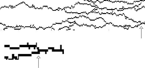
Figure 2: A space-time trajectory for the FA model in $1+1$ dimensions; time runs horizontally from left to right; space vertically. Mobile sites are black. The events corresponding to the diagrams in Fig. 1 can be clearly seen. The wandering of the excitation lines corresponds to diffusion; branching and coagulation events act to renormalize the excitation lines. In the lower left a coagulation event is shown enlarged.

IV RG analysis of the action

IV.1 Langevin equation of motion

By making stationary variations of the action (11) with respect to the response field $\bar{\phi}$, $\delta\mathcal{S}/\delta\bar{\phi}=0$, we obtain the Langevin equation of motion for the field $\phi$:

$$\partial_{t}\phi(t)=D_{0}\nabla^{2}\phi+r_{0}\phi-\lambda_{0}\phi^{2}+\eta(x,t),$$ (13)

where the noise $\eta$ satisfies $\left\langle\eta(x,t)\right\rangle=0$, and

$$\left\langle\eta(x,t)\eta(x^{\prime},t^{\prime})\right\rangle=2\left(v_{0}\phi-\lambda_{0}^{(2)}\phi^{2}\right)\delta(x-x^{\prime})\delta(t-t^{\prime}).$$ (14)

We neglect diffusive noise. The noise-noise correlator (14) describes stochastic fluctuations of the mobility field $\phi$, and comes from the coefficient of the terms in the action quadratic in $\bar{\phi}$. We see that (14) describes a competition between mobility correlations and anti-correlations, induced by branching and coagulation, respectively. If for example a branching event occurs, a particle will find itself with more nearest neighbours than one would expect from a mean-field argument. In the long time and wavelength limit, for $d\geq 2$, we show below that the second term in Eq. (14) is irrelevant, and may be dropped. Equations (13) and (14) then constitute the well-known Langevin equation for DP Hinrichsen , albeit with a positive definite mass term.

The mean-field approximation consists of dropping the noise and diffusion terms from (13). The resulting equation possesses a dynamic critical point at $c\propto r_{0}=0$, or $T=0$. For $T>0$, in the non-equilibrium regime, the density $\phi$ approaches its thermal expectation value $c=\rho/\gamma$ exponentially quickly. At $T=0$ the decay becomes algebraic, $\phi(t\to\infty)\sim\left(\lambda_{0}t\right)^{-1}$. Whether at equilibrium or not, the mean-field equation admits the critical exponents $\nu_{\parallel}=1$ and $\beta=1$. The former describes the growth of time scales $\xi_{\parallel}$ near criticality, via $\xi_{\parallel}\sim c^{-\nu_{\parallel}}$; the latter is the order parameter exponent, defined as the long-time scaling of the density in terms of the control parameter, $n(t\to\infty)\sim c^{\beta}$. By restoring the diffusive term, the spatial exponent $\nu_{\perp}=\frac{1}{2}$, defined analogously to $\nu_{\parallel}$, may be identified.

In the following section we show that fluctuations alter these predictions in low dimensions, by virtue of endowing space and time scale exponents with small dimension-dependent corrections. The exponent $\beta$, however, remains unchanged. We argue that because our model possesses detailed balance, which ensures that $\left\langle\phi(t\to\infty)\right\rangle\equiv\left\langle\phi\right\rangle=c$, this fixes $\beta$ to unity. This may also be inferred from the invariance of the unshifted action under the transformation $\left(\phi,\phi^{\star}\right)\to\left(c\phi^{\star},c^{-1}\phi\right)$, and the consequent Ward identity ZinnJustin .

IV.2 Dimensional analysis

We identify the upper critical dimension of the model via dimensional analysis Amit ; Tauber . We rescale space according to $x\rightarrow x\rho^{1/2}$, in order to remove the temperature dependence from the diffusion coefficient. Note that this rescaling is not valid at $c=0$. The action (11) then reads as before, with rescaled parameters $\lambda_{0}^{(1,2)}\equiv 2da^{d}\rho^{-\frac{d}{2}}\gamma$, $r_{0}=v_{0}\equiv 2d\rho$, $\sigma_{0}\equiv a^{2}$, and $\nu_{0}^{(1,2)}\equiv\gamma\rho^{-1-\frac{d}{2}}a^{d+2}$. We show some of the diagrams corresponding to these couplings in Fig. 3a.

Figure 3: Vertices corresponding to terms in the action (11). (a) From left to right, diagrams corresponding to the vertices $-\lambda_{0}^{(1)}$, $v_{0}$, $-\lambda_{0}^{(2)}$, and $\nu_{0}^{(1)}q_{1}^{2}$. The dot denotes a momentum dependence $q_{1}^{2}$ on one of the incoming legs. (b) The structure of the lowest-order corrections to the propagator, showing how the effective couplings emerge. The coupling shown here is $x$. Similar diagrams with dots on right, left and both vertices correspond to propagator renormalization controlled by the couplings $y$, $z$ and $u$, respectively. (c) Diagrams renormalizing the coupling $x$. Because these diagrams are symmetric with respect to incoming and outgoing momenta and frequencies, the contribution from each is doubled. Note that (b) also contributes to the renormalization of $x$, via the renormalization of $D$.

To perform a scaling analysis, we identify the effective couplings emerging from the action. These follow from the structure of the diagram shown in Fig. 3b, and are

$$x_{0}\equiv\frac{v_{0}\lambda_{0}^{(1)}}{D_{0}^{2}},y_{0}\equiv\frac{\sigma_{0}\lambda_{0}^{(1)}}{D_{0}^{2}},z_{0}\equiv\frac{v_{0}\nu_{0}^{(1)}}{D_{0}^{2}},u_{0}\equiv\frac{\sigma_{0}\nu_{0}^{(1)}}{D_{0}^{2}}.$$ (15)

The factors of $D_{0}$ come from the explicit evaluation of the integrals associated with the diagrams. To (15) we add $g_{0}\equiv\lambda_{0}^{(2)}/D_{0}$ and $h_{0}\equiv\nu_{0}^{(2)}/D_{0}$, which couple to four-point vertices: see Fig. 3. Dimensional analysis reveals that the upper critical dimension is 4, at which the most relevant coupling, $x_{0}$, is marginal. Renormalization effects must therefore be taken into account for $d<4$. Above $d=4$ the classical (fluctuation-free) predictions apply. Other couplings become relevant below $d=2$, and we shall therefore restrict our analysis to $2\leq d\leq 4$. Dimension $d=1$ is treated separately in Section V.

IV.3 DP fixed point

We employ the usual field-theoretic renormalization group scheme Amit ; ZinnJustin , using dimensional regularization in $d=4-\epsilon$ dimensions to identify the unphysical ultra-violet (UV: short time and distance) poles of the vertex functions $\Gamma^{(\bar{N},N)}$ of the theory. The vertex functions $\Gamma^{(\bar{N},N)}$ consist of all one-particle-irreducible diagrams with $\bar{N}$ outgoing and $N$ incoming amputated lines. Their UV poles result from exchanging a lattice model, which is regularised at short distances, for a continuum field theory, which is not. But by invoking universality, which says that the behaviour of a system approaching criticality is governed by a small number of relevant parameters, we recognise that the UV poles correspond to irrelevant microscopic degrees of freedom. By removing these poles we both render our theory finite, and, via scale-invariance and dimensional analysis, infer its physically important infra-red (IR: large time and distance) scaling Tauber . We shall work to one-loop order, and use dimensional regularization and minimal subtraction Amit .

We introduce the following renormalized counterparts of the fields and couplings appearing in (11):

$$\begin{array}[]{c}\phi_{R}=Z_{\phi}^{-1}\phi,\quad\bar{\phi}_{R}=\bar{\phi},\quad\lambda^{(1)}=Z_{\phi}^{2}Z_{\lambda}\lambda_{0}^{(1)}\mu^{d-2},\\ v=Z_{\phi}Z_{v}v_{0}\mu^{-2},\quad r=Z_{\phi}Z_{r}(r_{0}-r_{0c})\mu^{-2},\\ D=Z_{\phi}Z_{D}D_{0},\end{array}$$ (17)

where $r_{0c}$ is the additive counterterm introduced to cure the quadratic divergence of the vertex function $\Gamma^{(1,1)}$. We have introduced an arbitrary momentum scale $\mu$ in order to render the couplings dimensionless, and have chosen to allocate dimensions to the fields according to $[\bar{\phi}]=1,[\phi]=\mu^{d}$. The predictions of the theory must be independent of this allocation.

We define the multiplicative renormalization factors $Z$ as follows. From the propagator couplings, we fix mass, field and diffusion constant renormalization via

$$\left.\partial_{i\omega}\Gamma^{(1,1)}_{R}(\omega,q)\right|_{NP}=1,$$

$$\left.\partial_{q^{2}}\Gamma^{(1,1)}_{R}(\omega,q)\right|_{NP}=D,$$

$$-\Gamma^{(1,1)}_{R}(0,0)=r\mu^{2},$$ (18)

while for the couplings comprising $x_{0}$ we impose the conditions

$$\lambda^{(1)}=\frac{1}{2}\left.\Gamma^{(1,2)}_{R}(\omega,q)\right|_{NP}\mu^{d-2},$$

$$v=-\frac{1}{2}\left.\Gamma^{(2,1)}_{R}(\omega,q)\right|_{NP}\mu^{-2}.$$ (19)

The subscript $NP$ stands for ‘normalization point’, and is the value of the external momentum scale at which we evaluate the vertex functions. It can be chosen for convenience, provided that it lies outside the IR-singular region; we take $NP=(i\omega,q^{2},r)=(2D\mu^{2},0,0)$. Note that this choice corresponds to the system at criticality, which for finite $T$ is an approximation. For non-zero $T$ one must retain the mass term in the propagator. This leads to the emergence of an effective coupling that flows logarithmically to zero, signaling a crossover to a massive, classical fixed point. We will discuss this case in Section IV.5.

We first assume that for $2<d\leq 4$ the couplings other than $x_{0}$ are irrelevant, and hence the action (11) reduces to that of DP (we shall call $x$ the ‘DP coupling’). We shall find that those couplings which are marginal in $d=2$ at the classical fixed point are rendered irrelevant at the DP fixed point. Hence we expect to see DP scaling for $2\leq d\leq 4$. We find, to one-loop order, the well-known $Z$-factors Hinrichsen ,

$$Z_{\phi}=1+\frac{A_{d}}{4\epsilon}x_{0}\mu^{-\epsilon},\quad Z_{D}=1-\frac{A_{d}}{8\epsilon}x_{0}\mu^{-\epsilon},$$

$$Z_{r}=1-\frac{A_{d}}{2\epsilon}x_{0}\mu^{-\epsilon},\quad Z_{\lambda^{(1)}}=1-\frac{A_{d}}{\epsilon}x_{0}\mu^{-\epsilon},$$

$$Z_{v}=1-\frac{A_{d}}{\epsilon}x_{0}\mu^{-\epsilon},$$ (20)

where $A_{d}\equiv 4(4\pi)^{-d/2}\Gamma(3-d/2)$. Note that the cubic vertices renormalize identically as a consequence of a Ward identity. The renormalization factor associated with $x=\lambda^{(1)}v/D^{2}$ is therefore $Z_{x}=Z_{\phi}Z_{\lambda^{(1)}}Z_{v}Z_{D}^{-2}=1-(3A_{d}/2\epsilon)x_{0}\mu^{-\epsilon}+\mathcal{O}(\epsilon^{2})$. Insofar as one can ignore the propagator mass, the rescaled coupling $x\rightarrow A_{d}x=A_{d}Z_{x}x_{0}\mu^{-\epsilon}$ changes with the observation scale $\mu$ according to

$$\beta_{x}\equiv\mu\frac{\partial x}{\partial\mu}=x\left(-\epsilon+\frac{3}{2}x\right).$$ (21)

If we parameterize the change in the observation scale by $\mu\rightarrow\mu(\ell)=\mu\ell$, we can solve (21) for $x(\ell)$:

$$x(\ell)=\frac{x^{\star}}{\left(\frac{x^{\star}}{x(1)}-1\right)\ell^{\epsilon}+1}.$$ (22)

Thus $x\rightarrow x^{\star}\equiv 2\epsilon/3$ as $\ell\rightarrow 0$, because $\epsilon>0$. Since $\ell\approx 1$ and $\ell\ll 1$ correspond respectively to microscopic and macroscopic length and time scales, $x^{\star}$ is an IR-stable fixed point. At this fixed point the critical exponents of the theory are independent of its microscopic parameters, and so are ‘universal’. We therefore expect the model to display scaling behaviour independent of its microscopic details for very low temperatures. This scaling behaviour belongs to the universality class of directed percolation.

Having assumed the non-DP couplings in the action are irrelevant for $2<d\leq 4$, we shall now justify this assumption. These couplings are indeed irrelevant at the classical fixed point, as one can verify from (11) by dimensional analysis. We find that they remain irrelevant at the DP fixed point. Further, those couplings $(y,z,g)$ which are marginal in $d=2$ at the classical fixed point are rendered irrelevant at the DP fixed point. Hence we expect to see DP scaling in $d=2$, also. Defining a renormalization scheme in a similar manner to before,

$$\lambda^{(2)}=Z_{\phi}^{2}Z_{\lambda^{(2)}}\lambda_{0}^{(2)}\mu^{d-2},\quad\,\sigma=Z_{\phi}Z_{\sigma}\sigma_{0},\quad$$

$$\nu^{(1)}=Z_{\phi}^{2}\nu_{0}^{(1)}Z_{\nu^{(1)}}\mu^{d},\quad\,\nu^{(2)}=Z_{\phi}^{2}Z_{\nu^{(2)}}\nu_{0}^{(2)}\mu^{d},$$ (23)

where

$$\lambda^{(2)}=\left.\frac{1}{4}\Gamma^{(2,2)}_{R}(q,\omega)\right|_{NP}\mu^{d-2},$$

$$\sigma=\left.\partial_{q^{2}}\Gamma^{(2,1)}_{R}(q,\omega)\right|_{NP},$$

$$\nu^{(1)}=\left.\partial_{q^{2}}\Gamma^{(1,2)}_{R}(q,\omega)\right|_{NP}\mu^{d},$$

$$\nu^{(2)}=\left.\partial_{q^{2}}\Gamma^{(2,2)}_{R}(q,\omega)\right|_{NP}\mu^{d}.$$ (24)

we find to one-loop order

$$Z_{\nu^{(1)}}=Z_{\sigma}=1-\frac{2A_{d}}{\epsilon}x_{0}\mu^{-\epsilon},$$

$$Z_{\lambda^{(2)}}=1-\frac{A_{d}}{\epsilon}x_{0}\mu^{-\epsilon}.$$ (25)

The corrections to the Gaussian scaling dimensions of these couplings may then be calculated. The correction to the Gaussian eigenvalue of $g\equiv\lambda^{(2)}/D$ is determined by $Z_{g}=Z_{\phi}Z_{\lambda^{(2)}}Z_{D}^{-1}=1-5x_{0}\mu^{-\epsilon}/(8\epsilon)$. So $\gamma_{g}^{\star}\equiv\left.\mu\partial_{\mu}\ln(g/g_{0})\right|_{x=x^{\star}}=d-2+5\epsilon/12$. Thus $g$ is less relevant at the DP fixed point than at the Gaussian fixed point, and for $d\geq 2$ may safely be ignored. So too may $h$. In a similar way we find that $\gamma^{\star}_{y}=\gamma^{\star}_{z}=d-2+5\epsilon/3$, and $\gamma^{\star}_{u}=d+7\epsilon/3$, all of which are irrelevant for $d\geq 2$ at the DP fixed point. Thus for $2\leq d\leq 4$ the scaling properties of the model near criticality are those of DP.

The critical exponents of the model then follow from standard arguments Amit ; Hinrichsen . They are, to $\mathcal{O}(\epsilon)$, $\left(\nu_{\perp}^{DP},\nu_{\parallel}^{DP}\right)=\left(\frac{1}{2}+\frac{\epsilon}{16},1+\frac{\epsilon}{12}\right)$. The temporal exponent appropriate for comparing these predictions with numerical simulations is $1+\nu_{\parallel}$. The additional factor of unity arises because the microscopic timescale associated with the system goes itself as $\sim c$. The non-trivial value of $\beta$, $\beta^{DP}=1-\epsilon/6$, cannot be observed for a model such as ours which eventually equilibrates, as discussed above.

IV.4 Critical temperature

In general, systems in the DP universality class, such as directed bond percolation in $1+1$ dimensions, exhibit a continuous phase transition from an active to an absorbing state at some finite value $p_{c}\neq 0$ of their control parameter $p$. Our model, for which $p=c$, displays no such transition. One can justify this difference on physical grounds, as follows. If we interpret the mobility $n_{i}$ as the concentration of a chemical reactant $A$, then the KCM we study for $d>2$ corresponds to a chemical reaction involving diffusion $(A+\emptyset\leftrightarrow\emptyset+A)$, branching $(A+\emptyset\rightarrow A+A)$ and coagulation $(A+A\rightarrow A+\emptyset)$. Recall that the diffusive process arises from the mechanism of mobility creation facilitated by a nearest-neighbour site, and is made manifest only following a shift of the response field. DP corresponds to these three processes plus self destruction, $A+\emptyset\stackrel{{\scriptstyle\sigma_{0}}}{{\longrightarrow}}\emptyset+\emptyset$. It is self destruction that permits other systems in the DP universality class to undergo a phase transition at a finite value of the control parameter. Self destruction gives rise to a second-quantized operator

$$H_{sd}=-\sigma_{0}(a_{i}-a^{\dagger}_{i}a_{i}),$$ (26)

which, following a shift of the response field, results in a term in the action of the form $\sigma_{0}\bar{\phi}\phi$. Thus the mean-field critical point becomes $p_{c}=\sigma_{0}$. Near criticality, $p_{c}$ is increased above its mean-field value by fluctuations. This occurs because the DP noise-noise correlator is positive, and so coagulation is enhanced by the branching process: each particle finds itself with more neighbours with which it may coagulate than one would expect from a mean-field approximation. This enhanced coagulation enters the term which renormalizes the mass, effectively enhancing self-destruction relative to branching, and shifting the critical percolation threshold upwards.

Now self destruction is excluded by any dynamical rule preventing mobility destruction unless facilitated by a nearest neighbour. Moreover, no such process can be generated under renormalization from only branching and coagulation processes whose respective rates are fixed by detailed balance. Hence we expect one-spin facilitated models in general to have a critical point at zero temperature.

This argument may be made explicit for the model we study. By imposing the condition for criticality, $0=\Gamma^{(1,1)}(\omega=0,q=0,r_{0}=r_{0c})$, we find that, to one-loop order

$$r_{0c}=\frac{\left(\lambda_{0}v_{0}/D_{0}\right)\tilde{N}_{d}\Lambda^{d-2}}{1-\left(\lambda_{0}v_{0}/D_{0}^{2}\right)N_{d}\Lambda^{d-4}}.$$ (27)

Here, for convenience, we have imposed an explicit wavevector cutoff $\Lambda$; the additive correction to the mass is formally equal to zero in dimensional regularization, and yet the physical shift of the critical temperature must be independent of the regularization scheme used Tauber . We have introduced $N_{d}(2\pi)^{-d}(d-4)^{-1}\mathcal{S}_{d}$, where $\mathcal{S}_{d}\equiv 2\pi^{d/2}/\Gamma(d/2)$ is the surface area of a $d$-dimensional hypersphere, and $\tilde{N}_{d}\equiv(d-4)N_{d}/(d-2)$. We also use the unscaled variables of the action (11), in which $D_{0}\propto c$.

From (27) we see that the critical bare mass changes sign as $T\rightarrow 0$ from above. Ostensibly the critical temperature is then negative; physically, of course, it is zero. This is a consequence of the vanishing of fluctuations in the limit of zero temperature, which may be inferred from the vanishing in that limit of the branching vertex in the action. The diffusion term arises from nearest-neighbour-facilitated branching, and so must also vanish in this limit. Thus there is no fluctuation-induced shift of the critical temperature which remains $T_{c}=0$.

This is as we expect, if the field theory is a faithful representation of the original master equation. The master equation satisfies detailed balance at all temperatures, which means that it cannot admit an absorbing state: an absorbing state breaks detailed balance because it is a state that may be entered, but not left. Nonetheless, it is necessary to verify, as in Eq. (27), that there exists no finite-temperature absorbing state under coarse-graining of the master equation. The FA model, upon which the field theory is based, is known to have a critical point at zero temperature Ritort-Sollich .

IV.5 Crossover to classical behaviour

For any $T>0$ the mass parameter $r_{0}\propto c$ will be non-zero. Under renormalization, as discussed above, it will eventually become large, rendering our approximation of criticality incorrect. The system will thus for very large time and length scales exhibit classical scaling properties, with the associated simple exponents.

We can quantify the emergence of the classical theory by retaining the mass term in the propagator Cardy-et-al . If we write $s\equiv r/D$, we find that

$$\frac{d\ln x(\ell)}{d\ln\ell} =-\epsilon+\frac{3}{2}g(\ell),$$ (28)

$$\frac{d\ln s(\ell)}{d\ln\ell} =-2+\frac{3}{8}g(\ell),$$ (29)

where $g(\ell)\equiv x(\ell)(1+s(\ell))^{d/2-2}$ is an effective coupling. For small $s$, $x$ would in the IR limit approach to the directed percolation fixed point. But $s$ does not remain small, flowing as $s(\ell)\sim\ell^{-2+\mathcal{O}(\epsilon)}$. If we introduce the scaled mass $\sigma\equiv\left(1+s(1)^{-1}\ell^{2+\mathcal{O}(\epsilon)}\right)^{-1}$, we find that in the large mass limit $\sigma\to 1$ we obtain a logarithmically diminishing coupling,

$$g(\ell)\sim g(1)\left\{1+\frac{3}{16}(4+d)g(1)\ln\ell+\cdots\right\}^{-1}.$$ (30)

The vanishing of the effective coupling signals the re-emergence of a classical theory: because $g$ couples to diagrams renormalizing the propagator, its logarithmic vanishing results in a logarithmic crossover to classical exponents.

Thus we should see DP scaling provided that temperatures are small enough and time and length scales are not too large. The crossover temperature will be system dependent, because the prefactors of the flowing couplings are non-universal. For larger temperature or large enough length and time scales we expect to see a logarithmic crossover to a classical theory. This is characterised, in the nonequilibrium regime, by exponential decay to the steady state, and in general by classical scaling behaviour.

V Dimension $d=1$ and CDP

For $d=1$ DP scaling no longer holds. This is signaled in the field theory by the relevance of some of the non-DP couplings between $d=2$ and $d=1$, and the resulting profusion of uncontrollable singularities Amit . In this section we argue that in $d=1$ systems with single-spin isotropic facilitation, such as the FA model, belong instead to the universality class of compact directed percolation (CDP) Hinrichsen .

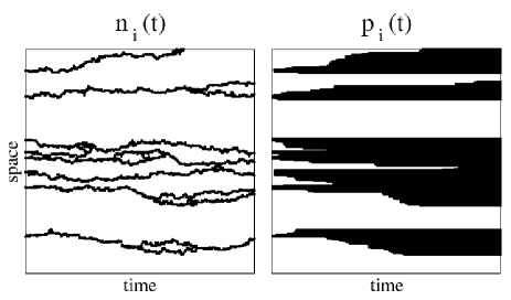
Figure 4: FA model in $d=1$. The left panel shows an equilibrium trajectory for the mobility field $n_{i}(t)$ at $T=0.3$ (window size is $L=250$ by $\Delta t=5000$). The right panel shows the corresponding trajectory of the persistence field $P_{i}(t)$; black sites denote those which have been or are mobile, and so satisfy $P_{i}(t)=0$. The clusters generated by the dynamics of the $P_{i}(t)$ are compact, and their scaling properties are that of CDP.

Consider the FA model in $d=1$. The elementary order parameter of this model is the mobility field $n_{i}(t)$. Figure 4 (left panel) shows a portion of an equilibrium trajectory at $T=0.3$. The connection between the FA model and CDP is made apparent by considering instead the corresponding persistence field $P_{i}(t)$, i.e. the field which takes value $P_{i}(t)=0$ if site $i$ has flipped by time $t$, and $P_{i}(t)=1$ otherwise. The corresponding trajectory of $P_{i}(t)$ in our example is shown in Fig. 4 (right panel).

Clearly, while the dynamics of $n_{i}(t)$ is reversible, that of $P_{i}(t)$ is not. A related observation is that the clusters generated by the evolution of $P_{i}(t)$ are compact, as seen in Fig. 4. The control parameter is again $c$, with $c=0$ corresponding to the transition between an active phase in which $P_{i}(t)$ eventually becomes unity throughout the whole system, and an inactive phase, in which it does not. As before, the exponents $\nu_{\parallel}$ and $\nu_{\perp}$ determine the scaling of times, $(D\tau)\sim c^{-\nu_{\parallel}}$ (with $D\approx c$), and lengths, $\xi\sim c^{-\nu_{\perp}}$. Two further exponents determine the asymptotic values of $\langle P_{i}(t)\rangle$. To extract these exponents it is convenient to define the transience function $T_{i}(t)\equiv 1-P_{i}(t)$: starting from an initial finite seed, $\langle T_{i}(t\to\infty)\rangle\sim c^{\beta}$, with the dynamics running in the forward time direction; starting from a completely full lattice, $\langle T_{i}(t\to-\infty)\rangle\sim c^{\beta^{\prime}}$, with the dynamics running backwards in time. Note that $\beta\neq\beta^{\prime}$ due to the irreversibility of $T_{i}(t)$ (or $P_{i}(t)$).

The domains of $T_{i}(t)$ spread only through diffusion of mobility excitations and interactions play no role. In this sense, the scaling behaviour of $T_{i}(t)$ should be that of freely-diffusing domain walls, and coalescing domains. Examples of systems which behave similarly are the zero temperature Ising chain under Glauber dynamics Hinrichsen , or the reaction-diffusion system $A+A\to\emptyset$ Peliti ; Hinrichsen . These indeed belong to the CDP universality class.

CDP has the following exponents Hinrichsen :

$$\nu_{\parallel}^{\rm CDP}=2,\;\;\;\nu_{\perp}^{\rm CDP}=1,\;\;\;\beta^{\rm CDP}=0,\;\;\;\beta^{\prime\rm CDP}=1\;.$$ (31)

These are precisely the values of the exponents of the FA model in $d=1$. The time and length exponents are $\nu_{\parallel}^{\rm FA}=2$ and $\nu_{\perp}^{\rm FA}=1$, giving the dynamic exponent $z^{\rm FA}\equiv\nu_{\parallel}^{\rm FA}/\nu_{\perp}^{\rm FA}=2$ Garrahan-Chandler ; Ritort-Sollich . Each site of a lattice which initially contains at least one excitation will eventually flip, and thus $T_{i}(t\to\infty)=1$ for all $i$, independently of $c$. We therefore have $\beta^{\rm FA}=0$, which is a consequence of ergodicity in the active phase. Conversely, if one takes a final state with all $T_{i}=1$, and runs time backwards, the state at $t\to-\infty$ will have a density of excitations, and therefore of $T_{i}$, equal to $c$. This is a consequence of detailed balance. Hence $\beta^{\prime\rm FA}=1=\beta^{\prime\rm CDP}$.

We propose a field-theoretic justification for this behaviour as follows. The Langevin equation of motion for $\phi$ is given by (13) and (14). At and above $d=2$ the term in $\lambda^{(2)}$ is irrelevant at the DP fixed point and may be dropped, leving us with the DP Langevin equation Hinrichsen . In $d=1$, however, at the DP fixed point (assuming it exists), we have from our previous results the anomalous dimensions of the couplings appearing in the noise correlator:

$$\gamma_{\lambda^{(2)}}^{\star}=d-2+\epsilon/3,\quad\gamma_{v}^{\star}=0.$$ (32)

We have calculated these dimensions using the prescription $[\bar{\phi}]=[\phi]=\mu^{d/2}$, appropriate when the cubic vertices are considered independently. We see that $\lambda^{(2)}$ and $v$ are both marginal in $d=1$. This is, we stress, a crude approximation, because the calculation of the anomalous dimensions assumes the irrelevance of $\lambda^{(2)}$. But it does suggest that here this assumption is inconsistent. Assuming that we can trust these exponents, there should then exist a fixed point controlled by $\lambda^{(2)}$, at which $v$ is irrelevant. Assuming this is so, and assuming further that the system can access this fixed point, this would leave the only vertices in the effective theory $\bar{\phi}\phi^{2}$ and $\left(\bar{\phi}\phi\right)^{2}$, which allow no propagator renormalization. Hence $z=2$ exactly. For this theory the beta function is calculable to all orders, since perturbation theory in $\lambda^{(2)}_{0}$ gives us a geometric series Peliti . We then have a new fixed point, at which there exists a renormalized value of $\lambda^{(1)}$ corresponding to an infinite value of its bare counterpart, $\lambda_{0}^{(1)}$. Thus $\lambda_{0}^{(1)}\phi^{2}\gg r_{0}\phi$, giving the effective theory

$$\partial_{t}\phi(t)=D_{0}\nabla^{2}\phi-\lambda_{0}^{(1)}\phi^{2}+i\sqrt{\lambda_{0}^{(2)}}\eta(x,t).$$ (33)

This is the Langevin equation for the CDP universality class Peliti . We stress that this argument is conjecture only. A more rigorous analysis of the field theory would be required in order to justify this claim.

VI Simulations of the $d=3$ FA model

The one-spin facilitated FA model Fredrickson-Andersen ; Ritort-Sollich is the lattice model upon which the field theory of the previous sections is based. In this section we report the results of our large-scale numerical simulations of the equilibrium dynamics of the FA model in dimension $d=3$, and compare these results to the predictions of the field theory. While the one dimensional FA model has been extensively studied by numerical simulations Ritort-Sollich , we are not aware of any detailed numerical study for $d>1$.

We consider the FA model on a cubic lattice with periodic boundary conditions. The model is defined by the Hamiltonian (1), and the isotropic dynamical rule

$$n_{i}=0\begin{array}[]{c}\xrightarrow{~{}~{}~{}{\mathcal{C}}_{i}~{}c~{}~{}}\\ \xleftarrow[{\mathcal{C}}_{i}~{}(1-c)]{}\\ \end{array}n_{i}=1.$$ (34)

The kinetic contraint is ${\mathcal{C}}_{i}=1-\prod_{\langle j,i\rangle}(1-n_{j})$, where $\langle j,i\rangle$ denotes nearest-neighbour pairs. We perform Monte-Carlo simulations of this model for several temperatures in the range $T\in[0.09,5.0]$. We use the continuous time algorithm Newman-Barkema , which is well-suited to this problem. The dynamical slow-down in this model is accompanied by the growth of a dynamic correlation length, and hence we must account for possible finite size effects. For instance, at $T=0.09$ it was necessary (and perhaps even then not sufficient: see below) to use system sizes as large as $N=160^{3}$.

VI.1 Global dynamics

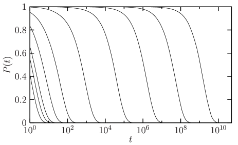
Figure 5: Persistence function $P(t)$ for the $d=3$ FA model. From left to right: $T=5.0$, 1.5, 1.0, 0.6, 0.4, 0.25, 0.17, 0.13, 0.106 and 0.009.

We first consider the spatially averaged dynamics. This may be probed via the mean persistence function,

$$P(t)=\left\langle\frac{1}{N}\sum_{i}P_{i}(t)\right\rangle,$$ (35)

where $P_{i}(t)$ is the single-site persistence function at time $t$, which takes value $1$ if site $i$ has not flipped up to time $t$, and value $0$ otherwise. Fig. 5 shows, as expected, that the dynamics slows down markedly when temperature is decreased below $T_{o}\approx 1.0$, which marks the onset of slow dynamics in this model Berthier-Garrahan ; Brumer-Reichman .

We extract the mean relaxation time, $\tau(T)$, via the usual relation $P(\tau)=e^{-1}$. The temperature dependence of $\tau$ is shown in Fig. 6, where various fits are also included. The high temperature behaviour is well described by a naive mean-field approximation Berthier-Garrahan ,

$$\tau_{MF}\sim c^{-1}.$$ (36)

This behaviour breaks down below $T_{o}$, where fluctuation-dominated dynamics becomes important. From our field theoretic arguments we expect that in the non-trivial scaling regime

$$\tau\sim c^{-\Delta},\quad\Delta=1+\nu_{\parallel}\approx 2.1,$$ (37)

where the numerical value is the DP estimate in three dimensions Hinrichsen . Fitting our data with the form $\tau\sim c^{-\Delta}$ we find

$$\Delta=2.095\pm 0.01,$$ (38)

as shown in Fig. 6. We include for comparison a fit using the Gaussian value of the exponent, $\Delta=2$, which is inconsistent with our data.

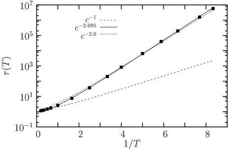
Figure 6: Arrhenius plot of the mean relaxation time in the $d=3$ FA model. The DP exponent fits the data, while the classical exponent does not.

We show in Fig. 7 the results for similar simulations of the FA model in dimensions $d$ from $1$ to $6$, together with the relevant DP exponent to $\mathcal{O}(\epsilon^{2})$, as tabulated in Ref. Hinrichsen . We note that these results are consistent also with numerical simulations of systems in the DP universality class Hinrichsen . Our numerics also show that one-spin facilitated FA models display, in all dimensions, Arrhenius behaviour. They are thus coarse-grained models for strong glass-formers, as expected Garrahan-Chandler-2 .

In summary, Fig. 7 strongly supports the RG prediction that the FA model exhibits non-classical scaling in low dimensions, consistent with DP behaviour for $d\geq 2$, and CDP behaviour in $d=1$.

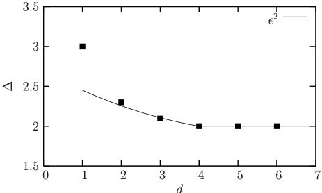
Figure 7: Dimensionality dependence of the time exponent $\Delta=1+\nu_{\parallel}$ of the FA model, from numerical simulations in dimensions $d=1$ to $d=6$ (filled squares). The full line is the $\epsilon^{2}$ expansion prediction. The values of the exponents agree within errorbars with those for DP for all $d>1$, and and CDP for $d=1$. The upper critical dimension of the FA model is $d_{c}^{FA}=d_{c}^{DP}=4$.

VI.2 Distribution of relaxation times

The mean relaxation time $\tau(T)$ captures only in part the relaxation behaviour of the model. We consider in this subsection the distribution of relaxation times, $\pi(t)$, related to the mean persistence function via Berthier-Garrahan

$$P(t)=\int_{t}^{\infty}dt^{\prime}\pi(t^{\prime}).$$ (39)

These distributions are shown in Fig. 8.

A careful study of the functions $P(t)$ and $\pi(t)$ reveals the following structure. At very large times, the persistence decays to 0 in a purely exponential manner, $P(t\gg\tau)\sim\exp(-t/\tau)$. This is not the case in $d=1$, where asymptotically the decay is described by a stretched exponential with stretching exponent $\beta=1/2$. That stretched exponential behaviour is not seen in $d=3$ is consistent with the fact that strong glass-formers display an almost-exponential relaxation pattern Angell .

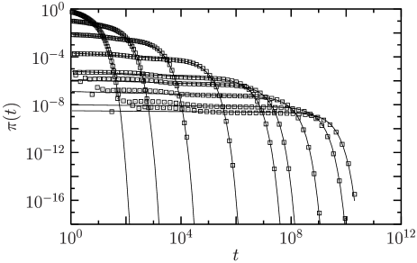
Figure 8: Distribution of relaxation times (symbols) and fits to Eq. (40) (full lines) for temperatures $T=1.0$, 0.4, 0.25, 0.17, 0.13, 0.12, 0.106, and 0.09 (from left to right).

Using $\tau(T)$ as a unique fitting parameter does not allow a satisfactory description of the whole decay of the persistence function: see Fig. 9. This figure shows that there exists an ‘additional short-time process’, in the language of glass transition dynamical studies.

Indeed, we find that fitting our data with the expression

$$\pi(t)\sim t^{-a}\exp\left(-\frac{t}{\tau}\right),$$ (40)

where $a$ and $\tau$ are free parameters, describes the distributions reasonably well over several decades: see Fig. 8.

Often, data in the supercooled liquid literature are presented in the frequency domain, because many decades can be accessed via e.g. dielectric spectroscopy nagel . Following this convention, we present frequency data obtained from the distribution of time scales via

$$P(\omega)=\int_{-\infty}^{\infty}\pi(\log(\tau))\frac{1}{1+i\omega\tau}\,d\log\tau.$$ (41)

Interestingly, the short-time power law behaviour $\pi(t)\sim t^{-a}$ observed in the distributions of time scales is also apparent in the frequency space as an ‘additional process’ on the high-frequency flank of the $\alpha$ relaxation, $P^{\prime\prime}(\omega)\sim\omega^{-1+a}$: see Fig. 9. In this figure, the full lines correspond to fits of the main peak with a simple exponential, as discussed above.

This feature is reminiscent of the ‘high-frequency wing’ discussed at length in the dielectric spectroscopy literature nagel . The wing is usually oberved in fragile glass-formers; unfortunately, no dielectric data is available for strong glass-formers leheny . Other techniques, such as Photon Correlation Spectroscopy, hint at the presence of an additional process in strong glass-formers similar to that observed in Fig. 9 strong . More experimental studies of the dynamics of strong glass-formers would be needed to confirm and quantify this similarity.

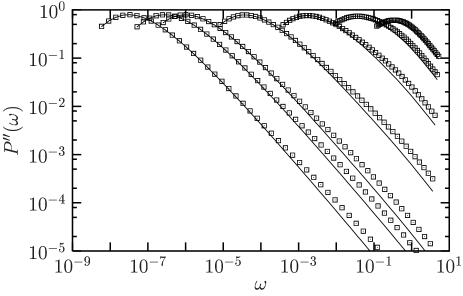
Figure 9: Top: The fit of the persistence function with a simple exponential reveals an additional short-time process. Bottom: This is also true in Fourier space, where the additional process looks like a ‘high-frequency wing’.

VI.3 Dynamic heterogeneity

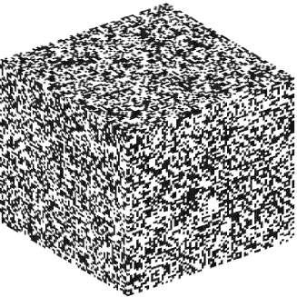
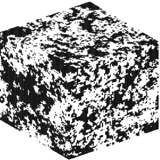
Figure 10: Spatial distribution of the local persistence at time $t^{\star}$ such that $P(t^{\star})=1/2$ (i.e., 50% of sites, shown in black, have flipped by time $t^{\star}$). From top to bottom, $T=1.0$, 0.2 and 0.12. The appearance of dynamic critical fluctuations when $T\to 0$ is evident.

The growth of timescales in the FA model, $\tau\sim c^{-\Delta}$, is accompanied by growing spatial correlations, $\xi\sim c^{-\nu_{\perp}}$, as the system approaches its critical point at $T=0$. These correlations are purely dynamical in origin, and give rise to dynamic heterogeneity Garrahan-Chandler ; Berthier-et-al . Figure 10 illustrates this phenomenon in the FA model. We quantify the local dynamics via the persistence function $P_{i}(t)$. For a given temperature we run the dynamics for a time $t^{\star}$, such that $P(t^{\star})=1/2$, meaning that half of the sites have flipped at least once. We colour white persistent (immobile) spins, for which $P_{i}(t^{\star})=1$, and black transient (currently or previously mobile) spins, for which $P_{i}(t^{\star})=0$. Figure 10 shows the persistence function for the $d=3$ FA model at different temperatures. Clearly, the dynamics is heterogeneous, and the spatial correlations of the local dynamics grow as $T$ is decreased. The ‘critical’ nature of dynamic clusters is apparent: the pictures are reminiscent of the spatial fluctuations of an order parameter close to a continuous phase transition, such as the magnetization of an Ising model near criticality. In our case, the order parameter is a dynamic object, the persistence function, and the critical fluctuations are purely dynamical in origin fss .

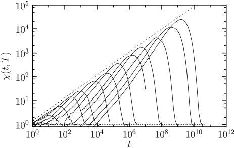
Figure 11: Time dependence of the dynamic susceptibility (43) at different temperatures. From left to right $T=1.0$, 0.6, 0.4, 0.3, 0.25, 0.2, 0.17, 0.15 and 0.13. The horizontal dotted line denotes the infinite time value, $\chi(t\to\infty)=1$; the diagonal dotted line denotes the power-law fit $\chi(\tau,T)\sim\tau^{0.46}$.

We now quantify these observations. We can measure spatial correlations of the local dynamics via a spatial correlator of the persistence function,

$$C(r,t,T)=\frac{1}{Nf(t)}\sum_{i}\Big{[}\langle P_{i}(t)P_{i+r}(t)\rangle-P^{2}(t)\Big{]},$$ (42)

where the function $f(t)=P(t)-P^{2}(t)$ in the denominator ensures the normalization $C(r=0,t,T)=1$. Alternatively, one can take the Fourier transform of (42), giving the corresponding structure factor of the dynamic heterogeneity,

$$S(q,t,T)=\frac{1}{Nf(t)}\sum_{k,l}\Big{[}\langle P_{k}(t)P_{l}(t)\rangle-P^{2}(t)\Big{]}e^{iq(k-l)}.$$

Finally, the zero wavevector limit of $S(q,t)$ defines a dynamic susceptibility, $\chi(t,T)=S(q=0,t,T)$, which can be rewritten as the normalized variance of the (unaveraged) persistence function, $p(t)\equiv N^{-1}\sum_{i}P_{i}(t)$:

$$\chi(t,T)=\frac{N}{f(t)}\big{[}\langle p^{2}(t)\rangle-\langle p(t)\rangle^{2}\big{]}.$$ (43)

Figure 11 shows the time dependence of the susceptibility (43) for various temperatures. The behaviour of $\chi$ is similar to that observed in atomistic simulations of supercooled liquids in general DHnum , and strong liquids in particular Vogel-Glotzer . The susceptibility develops at low temperature a peak whose amplitude increases, and whose position shifts to larger times as $T$ decreases. As expected, the location of the peak scales with the relaxation time $\tau(T)$, indicating that dynamical trajectories are maximally heterogeneous when $t\approx\tau(T)$.

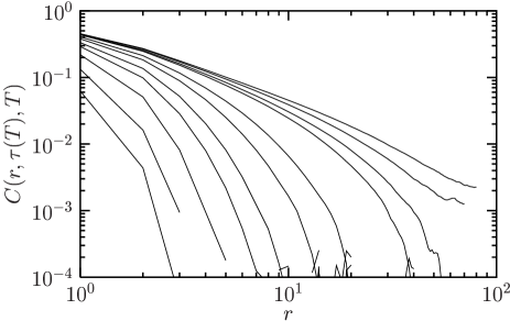
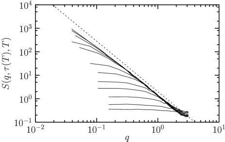
Figure 12: The spatial correlation function of dynamic heterogeneity in real (top panel) and Fourier (bottom panel) spaces reveals the growth of a dynamic length scale as $T\to 0$. Temperature decreases from left to right (top panel) and from bottom to top (bottom panel). The dashed line in the bottom panel denotes the asymptotic behaviour $S(q,\tau,T)\sim q^{-(2-\eta)}$, when $q\xi\gg 1$, with $\eta=-0.15$.

In Figure 12 we show the correlator $C(r,t,T)$ and the structure factor $S(q,t,T)$ for different temperatures and fixed times $t=\tau(T)$ where dynamic heterogeneity is maximal. These correlation functions clearly confirm the impression given by Fig. 10, that a dynamic length scale associated with spatial correlations of mobility develops and grows as $T$ decreases. Note that at the lowest temperatures the structure factor does not reach a plateau at low $q$. This because the system size we use, although very large ($N=160^{3}$), is not sufficiently so to allow us to probe the regime $q\xi\ll 1$. The necessary system sizes are simply too large to simulate on such long time scales.

We can extract numerically the value of the dynamic length scale, $\xi(T)$, at each temperature. To do so, we study in detail the shape of the correlation functions shown in Fig. 12. As for standard critical phenomena, we find that the dynamic structure factor can be rescaled according to

$$S(q,t,T)\sim\chi(\tau,T){\mathcal{S}}\left(q\xi\right),$$ (44)

where the scaling function $S(x)$ behaves as

$$S(x\to 0)\sim const$$ (45)

$$S(x\to\infty)\sim x^{2-\eta}.$$ (46)

Both the susceptibility $\chi$ and the dynamic length scale $\xi$ estimated at time $t=\tau$ behave as power laws of the defect concentration,

$$\chi\sim c^{-\gamma},\quad\quad\xi\sim c^{-\nu_{\perp}}.$$ (47)

These relations imply that the exponents $\gamma$ and $\nu_{\perp}$ should be numerically accessible by adjusting their values so that a plot of $c^{\gamma}S$ versus $qc^{-\nu_{\perp}}$ is independent of temperature. We show such a plot in Fig. 13, and we find that the values $\gamma\approx 0.97$ and $\nu_{\perp}\approx 0.5$ lead to a good collapse of the data. The exponent $\gamma$ can be independently and more directly estimated from Fig. 11 by measuring the height of the maximum of the susceptibility for various concentrations. Fitting the result to a power law of $c$ gives $\gamma\approx 0.96$, in reasonable agreement with the first value. We find also that the scaling function $S(x)$ is well-described by an empirical form $S(x)=1/(1+x^{2-\eta})$, consistent with Eq. (46). Thus we can determine the value of the ‘anomalous’ exponent, $\eta$; we find $\eta\approx-0.15$.

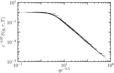
Figure 13: Collapse of the dynamic structure factor of Fig. 12 using scaling laws (47) and taking $\gamma=0.97$ and $\nu_{\perp}=0.5$. Dashed line is the scaling function $S(x)=1/(1+x^{2-\eta})$ with $\eta=-0.15$.

As usual, it is difficult to estimate what constitutes the ‘best’ collapse of the data, and so determine accurately the errors in the values of the exponents. Consequently, we are unable to determine $\nu_{\perp}$ with sufficient accuracy to conclude that it agrees—or disagrees—with the $d=3$ DP value, $\nu_{\perp}^{DP}\approx 0.58$. It is also difficult to compare $\gamma$ with its corresponding DP value, because this would require one to know the anomalous exponent $\eta$ characterizing spatial correlations of the persistence function. From a field theory perspective this is a formidable task. However, from our numerics we have that $\eta\approx-0.15$, and so from scaling arguments we find $\gamma=(2-\eta)\nu_{\perp}\approx 1.075$. This estimates lies however on the ‘wrong’ side of the classical value $\gamma^{cl}=1$ as compared to the numerical value obtained above.

We must conclude that numerical uncertainties are too large, and deviations from classical behaviour too small to make quantitative comparisons between DP and numerical exponents for spatial correlations. Plus, as we discussed above, our data may be subject at very low temperature to small, but unknown, finite size effects.

We are nonetheless satisfied that the naive estimate $\nu_{\perp}=1/d=1/3$ Ritort-Sollich that one gets by estimating the mean distance between defects is invalidated by our numerical results.

VII Conclusions

We have derived a field theory for a kinetically constrained model with isotropic facilitation, exemplified by the FA model. We have studied the field theory via RG, and the lattice-based FA model via numerical simulations. Our central results, briefly summarised in Ref. Whitelam-et-al , are the following.

The RG treatment suggests that the low-$T$ dynamics is dominated by a non-classical, zero-temperature critical point, which in turn implies that correlation times, dynamic correlation lengths and susceptibilities exhibit the scaling behaviour

$$\tau\sim c^{-\Delta},\;\;\;\xi\sim c^{-\nu_{\perp}},\;\;\;\chi\sim c^{-\gamma},$$ (48)

with $\Delta=1+\nu_{\parallel}$. The Arrhenius behaviour of the equilibrium concentration of excitations, $c\approx e^{-1/T}$, gives rise to Arrhenius behaviour of the dynamics through (48). For dimensions $d\geq 2$, the critical point is that of DP, while for $d=1$ it is that of CDP. The upper critical dimension is $d_{c}=4$, so that for dimensions $d\geq 4$ the exponents take classical values. For $d=d_{c}=4$ the exponents are classical, augmented with the usual logarithmic corrections Amit . For the time and space exponents we have Hinrichsen :

$$\Delta \approx 3,\,2.3,\,2.1,\,2\;\;\;\;\;(d=1,2,3,\geq 4),$$ (49)

$$\nu_{\perp} \approx 1,0\,.73,\,0.58,\,1/2.$$ (50)

We have also performed large-scale numerical simulations of the FA model, which confirm many of the field-theoretic predictions. The relaxation times of the FA model, Figs. 6 and 7, follow the scaling laws given by (48) and (49) in all dimensions simulated ($d=1$ to $6$). The existence of an upper critical dimension at $d_{c}=4$ is evident (see Fig. 7). The dynamics is increasingly heterogeneous and correlated in space as temperature is decreased, as can be seen, for example, in pictures of the local persistence (Fig. 10). The structure factor for this dynamic heterogeneity field in $d=3$ exhibits scale-invariance (Fig. 13).

More extensive simulations are required in order to clarify two further points. The spatial exponent obtained from the numerics is $\nu_{\perp}\sim 0.5$, but we were unable to establish whether this number agrees precisely with the $d=3$ DP value of $\nu_{\perp}=0.58$. We also caution the reader that there may exist, even for $d>2$, a crossover from early-time CDP behaviour to intermediate-time DP behaviour, as is the case for some systems in, ostensibly, the DP universality class Hinrichsen .

Our work shows that standard theoretical methods, such as the renormalization group, can be used to analyze coarse-grained models of glass-forming supercooled liquids fss ; steve . It supports the view that the dynamics of glass-formers is in many respects similar to that of standard critical phenomena, such as reaction-diffusion systems Tauber-review ; Lexie . We have found, numerically and analytically, that the FA model and its associated field theory possess a zero-temperature critical point, in agreement with results obtained by other means Ritort-Sollich . Rigorous results confirm the existence of a $T=0$ critical point in other kinetically contrained systems, such as the East model Aldous-Diaconis , and an analogous maximal-density critical point in the Kob-Andersen model Toninelli-et-al . Extending the field theory treatment to models of fragile glass-forming liquids, such as the East model Jackle and its generalizations Garrahan-Chandler-2 , constitutes an interesting challenge.

Finally, our results provide some insight into the physical meaning of fragility, in the Angell sense Angell . First, we have shown here and elsewehere Garrahan-Chandler ; Garrahan-Chandler-2 ; Berthier-Garrahan that strong systems show fluctuation-dominated heterogeneous dynamics, in a similar manner to fragile systems. This contradicts the popular view that ‘cooperativity’, ‘fragility’, and ‘heterogeneity’ are different facets of the same concept Ediger-et-al ; Angell .

In our view, the difference between strong and fragile liquids is in the strength of fluctuation effects. For example, the breakdown of the Stokes-Einstein relation observed in fragile liquids Chang-Sillescu ; Swallen-et-al should also be observed in strong ones Jung-et-al , but the effect will be less striking. However, since strong systems such as the FA model are characterized by a constant dynamic exponent, we expect that typical length scales at the glass transition are typically larger in strong glass-formers than in fragile ones. Detailed studies of dynamic heterogeneity in atomistic models of strong liquids should be able to test these predictions Vogel-Glotzer , while experimental investigations of strong glass-formers would also be very welcome.

- (1) M.D. Ediger, C.A. Angell and S.R. Nagel, J. Phys. Chem. 100, 13200 (1996).
- (2) C.A. Angell, Science 267, 1924 (1995).
- (3) P.G. Debenedetti and F.H. Stillinger, Nature 410, 259 (2001).
- (4) See for example, K. Schmidt–Rohr and H. Spiess, Phys. Rev. Lett. 66, 3020 (1991); R. Richert, Chem. Phys. Lett. 199, 355 1992; M.T. Cicerone and M.D. Ediger, J. Chem. Phys. 103, 5684 (1995); E.V. Russell and N.E. Israeloff, Nature 408, 695 (2000); L.A. Deschenes and D.A. Vanden Bout, Science 292, 255 (2001).
- (5) See for example, T. Muranaka and Y. Hitawari, Phys. Rev. E 51, R2735 (1995); D. Perera and P. Harrowell, Phys. Rev. E 51, 314 (1995); R. Yamamoto and A. Onuki, Phys. Rev. E 58, 3515 (1998). B. Doliwa and A. Heuer, Phys. Rev. Lett. 80, 4915 (1998); C. Donati, J.F. Douglas, W. Kob, S.J. Plimpton, P.H. Poole and S.C. Glotzer, Phys. Rev. E 60, 3107 (1999); C. Bennemann, C. Donati, J. Baschnagel and S.C. Glotzer, Nature 399, 246 (1999). N. Lacevic, F.W. Starr, T.B. Schrøder and S.C. Glotzer, J. Chem. Phys. 119, 7372 (2003).
- (6) M. Vogel and S.C. Glotzer, Phys. Rev. Lett. 92, 255901 (2004).
- (7) E. Weeks, J.C. Crocker, A.C. Levitt, A. Schofield, and D.A. Weitz, Science 287, 627 (2000); W. K. Kegel and A. van Blaaderen, Science 287, 290 (2000); E.R. Weeks and D.A. Weitz, Phys. Rev. Lett. 89, 095704 (2002).
- (8) H. Sillescu, J. Non-Cryst. Solids 243, 81 (1999).
- (9) M.D. Ediger, Annu. Rev. Phys. Chem. 51, 99 (2000).
- (10) S.C. Glotzer, J. Non-Cryst. Solids, 274, 342 (2000).
- (11) R. Richert, J. Phys. Condens. Matter 14, R703 (2002).
- (12) W. Götze and L. Sjögren, Rep. Prog. Phys. 55, 55 (1992).
- (13) M. Mézard and G. Parisi, Phys. Rev. Lett. 82, 747 (1999).
- (14) S. Franz and G. Parisi, J. Phys. C 12, 6335 (2000).
- (15) G. Biroli and J.-P. Bouchaud, Europhys. Lett. 67, 21 (2004).
- (16) G. Szamel, J. Chem. Phys. 121, 3355 (2004).
- (17) K.S. Schweizer and E.J. Saltzman, to appear in J. Phys. Chem. B (2004).
- (18) J.P. Garrahan and D. Chandler, Phys. Rev. Lett. 89, 035704 (2002).
- (19) D. Kivelson, S.A. Kivelson, X.L. Zhao, Z. Nussinov and G. Tarjus, Physica A 219, 27 (1995).
- (20) X. Xia and P.G. Wolynes, Proc. Natl. Acad. Sci. USA 97, 2990 (2000).
- (21) S. Whitelam, L. Berthier and J.P. Garrahan, Phys. Rev. Lett. 92, 185705 (2004).
- (22) J.P. Garrahan and D. Chandler, Proc. Natl. Acad. Sci. USA 100, 9710 (2003).
- (23) L. Berthier and J.P. Garrahan, J. Chem. Phys. 119, 4367 (2003); Phys. Rev. E 68, 041201 (2003).
- (24) S.H. Glarum, J. Chem. Phys. 33, 639 (1960).
- (25) G.H. Fredrickson and H.C. Andersen, Phys. Rev. Lett. 53, 1244 (1984).
- (26) R.G. Palmer, D.L. Stein, E. Abrahams and P.W. Anderson, Phys. Rev. Lett. 53, 958 (1984).
- (27) F. Ritort and P. Sollich, Adv. Phys. 52, 219 (2003).
- (28) For a review on directed percolation and related problems, see H. Hinrichsen, Adv. Phys. 49, 815 (2000).
- (29) V. Brunel, K. Oerding and F. van Wijland, J. Phys. A, 33, 1085 (2000).
- (30) M. Doi, J. Phys. A 9, 1465 (1976); L. Peliti, J. Physique 46, 1469, (1985).
- (31) B.P. Lee and J.L. Cardy, J. Stat. Phys. 80, 971, (1995); J.L. Cardy and U.C. Täuber, J. Stat. Phys. 90, 1, (1998).
- (32) D.C. Mattis and M.L. Glasser, Rev. Mod. Phys. 70, 979 (1998).
- (33) W. Kob and H.C. Andersen, Phys. Rev. E 48, 4364 (1993).
- (34) J. Jäckle and S. Eisinger, Z. Phys. B 84, 115 (1991).
- (35) U.C. Täuber, Adv. in Solid State Phys. 43, 659 (2003).
- (36) D.J. Amit, Field theory, the renormalization group, and critical phenomena (McGraw Hill, New York, 1984).
- (37) J. Zinn-Justin, Quantum Field Theory and Critical Phenomena (Oxford University Press, Oxford, 1989).
- (38) U.C. Täuber, Critical Dynamics: A field theory approach to equilibrium and non-equilibrium scaling behaviour, http://www.phys.vt.edu/tauber/utaeuber.html.
- (39) L. Peliti, J. Phys. A 19, L365 (1986).
- (40) M.E.J. Newman and G.T. Barkema, Monte Carlo Methods in Statistical Physics (Oxford University Press, Oxford, 1999).
- (41) Y. Brumer and D.R. Reichman, Phys. Rev. E 69, 041202 (2004).
- (42) P.K. Dixon, L. Wu, S.R. Nagel, B.D. Williams, and J.P. Carini, Phys. Rev. Lett. 65, 1108 (1990); U. Schneider, R. Brand, P. Lunkenheimer, and A. Loidl, Phys. Rev. Lett. 84, 5560 (2000); T. Blochowicz, C. Tschirwitz, S. Benkhof, and E.A. Rössler, J. Chem. Phys. 118, 7544 (2003).
- (43) R.L. Leheny, Phys. Rev. B 57, 10537 (1998).
- (44) D. Sidebottom, R. Bergman, L. Börjesson, and L.M. Torrel, Phys. Rev. Lett. 71, 2260 (1993); S.N. Yannopoulos, G.N. Papatheodorou, and G. Fytas, Phys. Rev. B 60, 15131 (1999).
- (45) L. Berthier, D. Chandler, and J.P. Garrahan, to be published.
- (46) L. Berthier, Phys. Rev. Lett. 91, 055701 (2003).
- (47) S. Whitelam and J.P. Garrahan, to appear in Phys. Rev. E, cond-mat/0405647.
- (48) L. Davison, D. Sherrington, J.P. Garrahan, A. Buhot, J. Phys. A: Math Gen. 34, 5147 (2001).
- (49) D. Aldous and P. Diaconis, J. Stat. Phys. 107, 945 (2002).
- (50) C. Toninelli, G. Biroli and D.S. Fisher, Phys. Rev. Lett. 92, 185504 (2004); C. Toninelli and G. Biroli, cond-mat/0402314.
- (51) I. Chang and H. Sillescu, J. Phys. Chem. B 101, 8794 (1997).
- (52) S.F. Swallen, P.A. Bonvallet, R.J. McMahon and M.D. Ediger, Phys. Rev. Lett. 90, 015901 (2003).
- (53) Y.J. Jung, J.P. Garrahan and D. Chandler, Phys. Rev. E 69, 061205 (2004).