Power law dependence of the angular momentum transition fields in few-electron quantum dots

Abstract

We show that the critical magnetic fields at which a few-electron quantum dot undergoes transitions between successive values of its angular momentum ($M$), for large $M$ values follow a very simple power-law dependence on the effective inter-electron interaction strength. We obtain this power law analytically from a quasi-classical treatment and demonstrate its nearly-universal validity by comparison with the results of exact diagonalization.

I Introduction

The field of quantum dots has been evolving under the busy attention of theorists and experimentalists alike for already almost 20 years by now.jacak98 ; maks00 ; kouw01 ; reimann02 This amount of interest and the enthusiasm is due to the unique blend of technological advances and fundamental interest. A special role is assigned to the magnetic field as a versatile tool with which one can tune the electronic properties of the quantum dots. In particular, the application of a perpendicular magnetic field aids the Wigner crystallization,mat_ssc ; reimann00 the formation of strongly correlated many-body statesjain95 ; kamilla95 and induces ground state multiplicity transitions.merkt91

From the theoretical side, the ‘exact’ numerical diagonalization methodmikh3 ; mikh3b ; mikh4 ; maarten03 ; yang93 ; eto97 ; yang02 ; reimann00 is of profound importance as a reference for approximate treatments. With the presently available computing power this approach has been successfully applied to compute the electronic structure of few-electron quantum dots. However, this method also has sharp limitations since the numerical effort grows exponentially with the number of electrons. Therefore, the construction, refinement and application of less demanding approximate approaches based on some enlightening or visualizing idea is of critical importance.

Among such ideas is the successful introduction of quasiparticles that came to be known as composite fermions.cf ; jain90 This transformation reduces the initial problem to a much more tractable problem of non-interacting or, at least, weakly interacting particles. Another fruitful idea is to gain insight from the classical picture. The electrons in a quantum dot can be viewed as classical particles vibrating around their equilibrium positionsbed94 ; matulis94 ; me98 not unlike atoms in a molecule or a solid, while the molecule can rotate as a whole.maks96 These developments culminated in the formulation of the rotating electron molecule approachyann02 ; yann03 based on a classical visualization and successfully competing with the composite fermion model.

In the present work, we call attention to yet another manifestation of the classical nature of quantum dots in strong magnetic fields. Namely, we concentrate on the critical magnetic fields, i. e. the field strengths at which the ground-state angular momentum of the dot switches between its two successive values. Here, we found that these critical field values show a strikingly simple dependence on the effective Coulomb coupling strength. We compare estimates extracted from an unsophisticated quasi-classical model with the exact-diagonalization results thereby demonstrating the viability of such essentially classical paradigms and presenting one more argument in their favor.

The paper is organized as follows. In Sec. II we present the exact-diagonalization results indicating that the critical magnetic fields obey a simple power law. In Sections III and IV we introduce and solve a simple quasi-classical model, and compare its predictions to the exact results in Sec. V. The paper ends with a concluding Sec. VI.

II Exact diagonalization

In Fig. 1 the well-known energy spectrum of two electrons in a parabolic dotmerkt91 (the Zeeman energy is not included) is plotted as a function of the perpendicular magnetic field strength $B$. We work with dimensionless variables so that the system energy is measured in units of $\hbar\omega_{0}$ with $\omega_{0}$ being the characteristic frequency of the confinement potential, while the magnetic field strength is expressed as the ratio $\gamma=\omega_{c}/\omega_{0}$ of the cyclotron frequency $\omega_{c}=eB/mc$ to the above-introduced confinement frequency. The relative importance of the electron-electron Coulomb interaction is characterized by the dimensionless coupling constant $\lambda=a_{0}/a_{B}$. Here $a_{0}=\sqrt{\hbar/m\omega_{0}}$ is the characteristic dimension of the parabolic quantum dot, and $a_{B}=\epsilon\hbar/me^{2}$ is the Bohr radius. Fig. 1 corresponds to a relatively large (i. e. strongly interacting) dot of $\lambda=5$, and we include the magnetic fields up to $\gamma=4$ and angular momenta up to $|M|=5$. We observe that for positive magnetic fields the preferred values of the angular momentum are negative, however, for the sake of convenience we will henceforth use the symbol $M$ for its absolute values and dispense with the “$-$” sign.

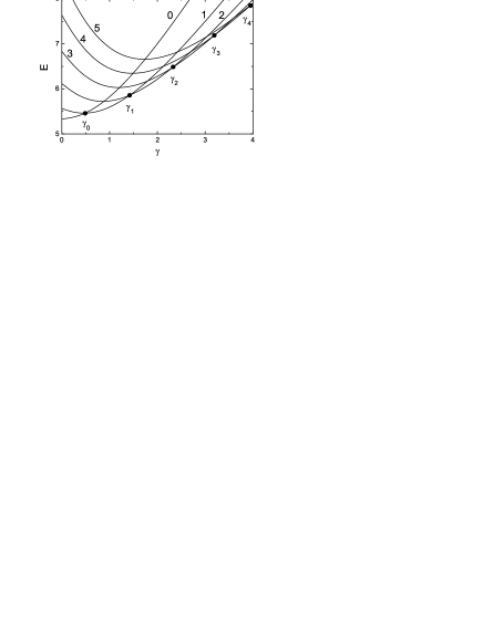
Figure 1: The spectrum of a strongly interacting ($\lambda=5$) two-electron parabolic dot as a function of perpendicular magnetic field. The lowest term of each angular momentum $M=0\ldots 5$ is shown. The Zeeman energy is not included. At the critical fields $\gamma_{M}$ the angular momentum switches from $M$ to $M+1$.

The most conspicuous feature of this spectrum is the presence of certain critical values $\gamma_{M}$ at which the ground state of the quantum dot changes the absolute value of its total angular momentum from $M$ to $M+1$. This feature is brought about by the electron-electron interaction and persists for any number of electrons in the dot.

We performed exact numerical diagonalization for quantum dots containing $2$, $3$ and $4$ electrons (see Ref. maarten03, for the description of the procedure) and calculated the critical magnetic field values for various effective Coulomb interaction strengths. For the two-electron quantum dot we included $\lambda$ values up to $20$, and for the case of three electrons in the dot the upper limit was set at $\lambda=10$. The case of four electrons is numerically more demanding and we restricted the calculation to values up to $\lambda=2$. We note that the effective electron-electron interaction strength can be easily tuned by varying the strength of the confinement potential, and consequently, the quantum dot size. In Figs. 2–4 these critical magnetic field values are shown in a double-logarithmic plot as a function of the dimensionless coupling constant $\lambda$. We display the magnetic field range between $\ln\gamma=0$ (that is, $\omega_{c}=\omega_{0}$) and $\ln\gamma=3$ ($\omega_{c}\approx 20\,\omega_{0}$).

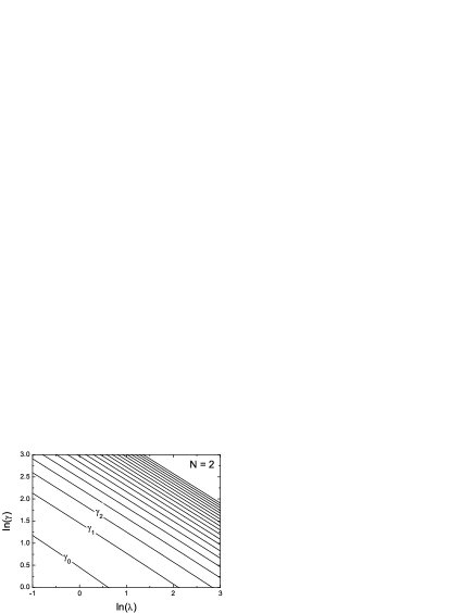
Figure 2: Critical magnetic field strength values for two electrons. The full lines delimit regions characterized by different ground-state angular momenta starting with $M=0$ at the lower left corner and increasing in steps of $\Delta M=1$ at each consecutive boundary. Note the monotonic decrease of inter-line distances with increasing $\lambda$ and $\gamma$.

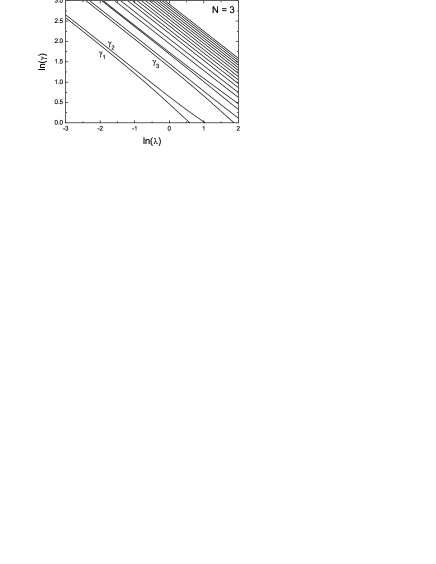
Figure 3: The same as in Fig. 2 but now for three electrons. An additional phase boundary separating regions of angular momentum $M=0$ and $M=1$ that shows a different behavior is not shown. Note that widths of some regions corresponding to more stable states are considerably larger.

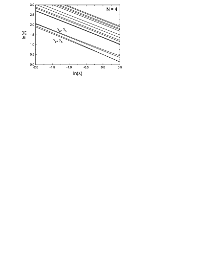
Figure 4: The same as in Fig. 2 but now for four electrons. An additional phase boundary separating regions of angular momentum $M=0$ and $M=2$ that shows a different behavior is not included. The regions corresponding to more stable states are wider.

Notice that plotted in a a logarithmic scale these functions are nearly linear, besides the linearity is more pronounced for large momentum $M$ and large magnetic field values. This linearity of the above curves

$$\ln\gamma_{M}=a_{M}+b_{M}\ln\lambda$$ (1)

implies the simple power law dependence

$$\gamma_{M}\propto\lambda^{b_{M}}.$$ (2)

We expect that such a plain dependence is a consequence of the classical nature of the electron system in the quantum dot in the limit of a strong perpendicular magnetic field (see e. g. Ref. dresden, ) as we will show in the next section where a simple quasi-classical description is developed.

We observe that the phase diagram corresponding to the two-electron quantum dot (Fig. 2) is more regular that the two others, namely, the nearly-straight-line boundaries appear to be parallel and the widths of the consecutive regions are decreasing monotonically. In contrast, the plots pertaining to the cases of three (Fig. 3) and four (Fig. 4) electrons include some regions of considerably larger width which indicate an enhanced stability of the corresponding ground states. In particular, such regions correspond to the maximum density droplet states of angular momentum $M=3$ for three electrons and $M=6$ for four electrons.

Moreover, we see that at the lower right corner of Figs. 3 and 4 (three and four electrons, respectively) corresponding to low magnetic fields and strong Coulomb coupling there is a slight deviation from collinearity between neighboring lines. In the case of the four-electron dot the phase boundaries $\gamma_{2}$ and $\gamma_{3}$ even merge together indicating that for $\ln\lambda>-0.3$ there is a direct transition from the state with $M=2$ into the state with $M=4$. Similar transitions where the angular momentum changes by $\Delta M=2$ were also found for higher values of angular momentum, namely, there are transitions $10\to 12$ and $12\to 14$. These properties of the four-electron quantum dot were already pointed out and discussed in Ref. maarten03, . As we will see shortly, the quasi-classical model will overlook the presence of such irregularities.

We note that in each of Figs. 3 and 4 an extra phase boundary is present at low magnetic fields which was omitted. These disregarded boundaries — see Fig. 2(a) of Ref. mikh3b, and Fig. 3 of Ref. maarten03, for phase diagrams of three- and four-electron systems, respectively — display a different trend. They are of a purely quantum-mechanical nature and result from a specific distribution of particles among the low-energy levels of a quantum dot, i. e. they are effects that can not be reproduced in a classical model.

III Quasi-classical description

The 2D $N$-electron system confined by a parabolic quantum dot and placed in a perpendicular magnetic field $B$ is described by the following dimensionless Schrödinger equation:

$$\{H-E\}\Psi=0,$$ (3)

where

$$H = \frac{1}{2}\sum_{n=1}^{N}\left\{\left(-i\nabla_{n}+\frac{\gamma}{2}[\mathbf{e}_{z}\times\mathbf{r}_{n}]\right)^{2}+r_{n}^{2}\right\}$$ (4)

$$+\sum_{n,m=1\atop n<m}^{N}\frac{\lambda}{|\mathbf{r}_{n}-\mathbf{r}_{m}|}.$$

We consider the ground state energy of the state of fixed angular momentum $M$ as a function of Coulomb coupling constant $\lambda$ and the magnetic field $\gamma$

$$E=E(\lambda,\gamma,M).$$ (5)

Solving the equation

$$E(\lambda,\gamma,M)=E(\lambda,\gamma,M+1)$$ (6)

for $\gamma$ will define the above-introduced critical magnetic field values $\gamma_{M}$ corresponding to the angular momentum transitions from $M$ to $M+1$.

It is well known that in the strong magnetic field regimemaks96 the electrons form a Wigner crystal which for a system up to five electrons is just a ring of equidistantly placed electrons.bed94

Due to the rotational symmetry around the $z$-axis the Hamiltonian (4) commutes with the total angular momentum operator

$$\hat{M}=-i\sum_{n=1}^{N}\frac{\partial}{\partial\varphi_{n}}.$$ (7)

Therefore, the simplest way to calculate the ground energy of the system is to exclude the magnetic field from the Schrödinger equation (3) by means of the transformation

$$\Psi\to\exp\left(i\sum_{n=1}^{N}\varphi_{n}/N\right)\Psi,$$ (8)

with the ensuing scaling of coordinates

$$\mathbf{r}_{n}\to\mathbf{r}_{n}\left(1+\gamma^{2}/4\right)^{-1/4},$$ (9)

which enables to transform the initial problem into the equivalent problem

$$\{\tilde{H}-E_{0}(\lambda_{0},M)\}\Psi=0$$ (10)

with the Hamiltonian

$$\tilde{H}=\frac{1}{2}\sum_{n=1}^{N}\left\{-\nabla_{n}^{2}+r_{n}^{2}\right\}+\sum_{n,m=1\atop n<m}^{N}\frac{\lambda_{0}}{|\mathbf{r}_{n}-\mathbf{r}_{m}|}.$$ (11)

without a magnetic field.

The coupling constants and the eigenvalues of both problems are related as

$$\lambda = \lambda_{0}\left\{1+(\gamma/2)^{2}\right\}^{1/4},$$ (12a)

$$E(\lambda,\gamma,M) = E_{0}(\lambda_{0},M)\sqrt{1+(\gamma/2)^{2}}-\gamma M/2.$$

Here, we again used our earlier convention whence the symbol $M$ stands for the absolute value of the angular momentum. Note that the eigenvalue $E_{0}(\lambda_{0},M)$ indeed depends only on the absolute value of the angular momentum, and Eq. (12) is written in accordance with our previous convention for $M$. Combining Eqs. (12) and (6) we arrive at the following equation

$$\frac{\gamma_{M}}{2\sqrt{1+(\gamma_{M}/2)^{2}}}=E_{0}\left(\lambda_{0},M+1\right)-E_{0}\left(\lambda_{0},M\right)$$ (13)

which expresses the critical magnetic field values in terms of the reduced problem (10).

IV Derivation of the power law dependence

Now we turn to the solution of the eigenvalue problem defined by Eq. (10) which involves two peculiar features. One is that we need to solve for a highly excited state with a large angular momentum $M$ that corresponds to the ground state of the original problem (3), and this fact complicates the solution. Also, according to Eq. (12a), in the strong magnetic field limit Eq. (10) has to be solved for small values of the coupling constant $\lambda_{0}$. Therefore, the solution must be attainable by means of some perturbative technique.

Neglecting the electron-electron interaction term in the Hamiltonian (11) we obtain the zero order equation. Due to the rotational symmetry the following radial equation for the zero-order one-electron function can be written:

$$\left\{-\frac{1}{2r}\frac{d}{dr}r\frac{d}{dr}+\frac{m^{2}}{2r^{2}}+\frac{1}{2}r^{2}-\varepsilon_{0}(m)\right\}\psi_{0}(m|r)=0.$$ (14)

Here, the symbol $m$ stands for the single-electron angular momentum. As this angular momentum is large the eigenvalue can be estimated by approximating the effective potential

$$V_{\mathrm{eff}}(r)=\frac{m^{2}}{2r^{2}}+\frac{1}{2}r^{2}$$ (15)

by a parabolic potential in the vicinity of its minimum at

$$r_{0}=|m|^{1/2}.$$ (16)

Here we disregard the first-derivative term in Eq. (14) as its inclusion gives only negligible corrections in the $m\to\infty$ limit. This leads to the following estimate for the one-electron energy

$$\varepsilon_{0}(m)\approx V_{\mathrm{eff}}(r_{0})=|m|,$$ (17)

and the total zero-order energy of all electrons in the dot becomes

$$E_{0}=N|m|=M.$$ (18)

Let us now estimate the characteristic energies of the two possible types of motion of the electrons: the radial vibrations and the motion of electrons along the ring.

The energy of the radial vibrations can be obtained by expanding the effective potential at the equilibrium point $r_{0}$. The second derivative of the potential

$$V_{\mathrm{eff}}^{\prime\prime}(r_{0})=4$$ (19)

is of order unity and does not depend on the orbital momentum $m$. This fact enables us to disregard these vibrations as their energy is small in comparison to the zero order energy $\varepsilon_{0}(m)$. Moreover, these vibrations are the same for any orbital momentum $M$ (they are not affected by the electron-electron interaction which is even smaller, i. e.  $\lambda/r_{0}\ll 1$), and thus they can be neglected when solving Eq. (13).

The energy of the longitudinal electron excitations along the ring is even smaller. Actually, in zero order approximation the electron state under consideration is degenerate with respect to these excitations since the same total energy of the electronic ring (18) can be constructed from various angular momentum distributions among individual electrons. Thus, this angular motion is highly affected by the weak electron-electron interaction. The result of this effect is well-know: it leads to the Wigner crystallization of the electrons along the ring.

The first order correction to the eigenvalue $E_{0}\left(\lambda_{0},M\right)$ is obtained by including the electron-electron interaction term, but calculated classically for the electrons positioned equidistantly on a ring of radius $r_{0}$. This energy correction reads

$$\Delta E(\lambda_{0},M)=\frac{\lambda_{0}}{r_{0}}f_{N}=\lambda_{0}\sqrt{\frac{N}{M}}\,f_{N},$$ (20)

where $f_{N}$ is the Coulomb energy of the equidistantly located electrons on the unit radius ring, in particular,

$$f_{2}=1/2,\quad f_{3}=\sqrt{3},\quad f_{4}=1+2\sqrt{2}.$$ (21)

Then, combining Eqs. (18) and (20) we obtain the final expression for the energy to first order in powers of $\lambda_{0}$

$$E(\lambda_{0},M)=M+\lambda_{0}\sqrt{\frac{N}{M}}\,f_{N}.$$ (22)

Inserting this expression into Eq. (13), solving it to the lowest accuracy in $\gamma^{-1}$ powers, and taking the average of the difference of two inverse square roots we obtain the result

$$\gamma=\frac{2}{(Nf_{N}^{2})^{1/3}}\left(M+\frac{1}{2}\right)\lambda^{-2/3}.$$ (23)

Finally, taking the logarithm of Eq. (23) and comparing to Eq. (1) we extract the expressions for the coefficients

$$a_{M} = \ln(2M+1)-\frac{1}{3}\ln N-\frac{2}{3}\ln f_{N},$$

$$b_{M} = -\frac{2}{3}.$$ (24)

V Comparison with the exact numerical results

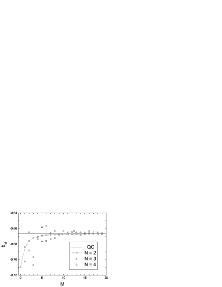
Figure 5: The power law coefficients $b_{M}$ as a function of the angular momentum $M$. The quasi-classical (QC) treatment predicts a universal value $b_{M}=-2/3$ for any number of electrons shown by the solid line. Different symbols indicate the exact values of the coefficients for quantum dots containing $2$ to $4$ electrons. The two-electron result displays a monotonic behavior and is spline-approximated by the dotted line to guide the eye.

The quasi-classical solution predicts a universal value for the power-law index $b_{M}=-2/3$ independent of the number of electrons. The comparison with the exact diagonalization results is displayed in Fig. 5. As discussed above, in the four-electron dot we encountered two cases when a single $\Delta M=2$ transition occurs in place of expected two $\Delta M=1$ transitions in the whole considered range of $\lambda$ and $\gamma$ values. In these cases (namely, the transitions $10\to 12$ and $12\to 14$) we used the $M$-value corresponding to the average of the two expected $\Delta M=1$ transitions.

In general, the discrepancy with our analytical model is small as all results fall into a range between $-0.64$ and $-0.72$. As expected, the deviation of the exact result from the quasi-classical limit rapidly decreases with increasing angular momentum $M$, and already at $M=8$ the difference is less than $2\%$.

The exact results corresponding to the two-electron dot show a monotonous behavior as indicated by the dotted-line in Fig. 5. The reason is that the two-electron system in a parabolic dot possesses only one non-trivial degree of freedom as the centre-of-mass motion can be separated from the relative motion and is not excited in the ground state. In contrast, the internal motion of three- and four-electron dots involves more degrees of freedom and is more intricate. This results in a more complicated dependence of $b_{M}$ on the angular momentum $M$. In particular, enhanced non-monotonicities are discernible in the vicinity of more stable maximum-density-droplet or “magic” states at $M=3$ and $6$ for three electrons and $M=6$ for four electrons.

Fig. 6 shows the comparison for the coefficient $a_{M}$. The quasi-classical model (IV) predicts a logarithmic dependence of $a_{M}$ on the angular momentum $M$. We see that for the two-electron system the correspondence is nearly perfect.

Figure 6: The coefficient $a_{M}$ as a function of the angular momentum for the case of $N=2$, $3$ and $4$ electrons in the dot. The full lines denote the quasi-classical (QC) result, and the symbols correspond to the results from exact-diagonalization.

The behavior concerning three and four electrons is more complex. At low values of the angular momentum (and thus low magnetic fields) there are notable discrepancies between the these sets of results in Fig. 6. In particular, we observe wide “gaps”, i. e. abrupt jumps in the $a_{M}$ values obtained from the exact-diagonalization at angular momenta $M=3$ ($M=6$) corresponding to maximum density droplet states in three (four) electron systems. Nevertheless, the overall trend of these dependences still follows the quasi-classical prediction rather closely, and the discrepancy between the classical and fully quantum mechanical results vanishes very quickly with increasing $M$.

VI Conclusions

In conclusion, we presented a quasi-classical theory of the magnetic properties of few-electron quantum dots whose main result is a simple power law dependence of the critical magnetic fields on the Coulomb coupling constant. While the main virtue of this theory lies in its relative simplicity and ability to provide results without resorting to heavy computation, the comparison of its predictions to the exact results also proves its robustness even in the realm of quantum mechanics.

- (1) L. Jacak, P. Hawrylak, and A. Wójs, Quantum Dots (Springer, Berlin, 1998).
- (2) P. A. Maksym, H. Imamura, G. P. Mallon, and H. Aoki, J. Phys.: Condens. Matter 12, 299 (2000).
- (3) L. P. Kouwenhoven, D. G. Austing, and S. Tarucha, Rep. Prog. Phys. 64, 701 (2001).
- (4) S. M. Reimann and M. Manninen, Rev. Mod. Phys. 74, 1283 (2002).
- (5) S. M. Reimann, M. Koskinen, and M. Manninen, Phys. Rev. B62, 8108 (2000).
- (6) A. Matulis and F. M. Peeters, Solid State Commun. 117, 655 (2001).
- (7) J. K. Jain and T. Kawamura, Europhys. Lett. 29, 321 (1995).
- (8) R. K. Kamilla and J. K. Jain, Phys. Rev. B52, 2798 (1995).
- (9) U. Merkt, J. Huser, and M. Wagner, Phys. Rev. B43, 7320 (1991).
- (10) S. A. Mikhailov, Phys. Rev. B65, 115312 (2001).
- (11) S. A. Mikhailov and N. A. Savostianova, Phys. Rev. B66, 033307 (2002).
- (12) S. A. Mikhailov, Phys. Rev. B66, 153313 (2002).
- (13) M. B. Tavernier, E. Anisimovas, F. M. Peeters, B. Szafran, J. Adamowski, and S. Bednarek, Phys. Rev. B(to be published 15 November 2003).
- (14) S.-R. E. Yang, A. H. MacDonald, and M. D. Johnson, Phys. Rev. Lett. 71, 3194 (1993).
- (15) M. Eto, Jpn. J. Appl. Phys. 36, 3924 (1997).
- (16) S.-R. E. Yang and A. H. MacDonald, Phys. Rev. B66, 041304 (2002).
- (17) J. K. Jain, Phys. Rev. B41, 7653 (1990); ibid. 42, 9193(E) (1990).
- (18) Composite Fermions: a unified view of the quantum Hall regime, editted by O. Heinonen (World Scientific, Singapore, 1998).
- (19) V. M. Bedanov and F. M. Peeters, Phys. Rev. B49, 2667 (1994).
- (20) A. Matulis and F. M. Peeters, J. Phys.: Condens. Matter 6, 7751 (1994).
- (21) E. Anisimovas and A. Matulis, J. Phys.: Condens. Matter 10, 601 (1998).
- (22) P. A. Maksym, Phys. Rev. B53, 10 871 (1996).
- (23) C. Yannouleas and U. Landman, Phys. Rev. B66, 115315 (2002).
- (24) C. Yannouleas and U. Landman, Phys. Rev. B68, 035326 (2003).
- (25) A. Matulis, in Nano-Physics and Bio-Electronics: a New Odyssey, editted by T. Chakraborty, F. Peeters, and U. Sivan (Elsevier, 2002), pp. 237-255.