Cavity polaritons: Classical behaviour of a quantum parametric oscillator

Abstract

We address theoretically the optical parametric oscillator based on semiconductor cavity exciton-polaritons under a pulsed excitation. A “hyperspin” formalism is developed which allows, in the case of large number of polaritons, to reduce quantum dynamics of the parametric oscillator wavefunction to the Liouville equation for the classical probability distribution. Implications for the statistics of polariton ensembles are analyzed.

I Introduction

Semiconductor microcavities with embedded quantum wells exhibit a rich variety of unusual light-matter coupling effects. In the strong coupling regime excitons and photons are mixed into a new kind of quasiparticles, known as cavity exciton-polaritons 1 . These particles inherit sharp energy dispersion of cavity photons and strong interaction nonlinearities of excitons. The bosonic nature of cavity polaritons allows to observe a number of coherent phenomena such as stimulated scattering of exciton-polaritons and even, perhaps, their Bose-condensation 2 ; 3 .

A non-parabolic shape of the lower dispersion branch of exciton-polaritons having a sharp mininum and flat wings allows for the so called parametric process when a pair of polaritons from the pump scatter into the signal and idler states with both energy and momentum conserved 3 ; 4 ; 5 (see Figure 1). The parametric scattering process was studied in detail experimentally under continuous-wave (cw) pumping in Refs. 6, ; 7, ; 8, ; 9, and under pulsed excitation in Refs. 10, ; 11, ; 12, . Previous theoretical treatment was based on the Heisenberg equations 13 ; 14 ; 15 . The quantum state of the “pumped” polaritons has been described by a classical non-fluctuating field which is valid only in the case of cw pumping. This approach allowed to obtain a closed set of equations, describing parametric amplification. However, effects of the parametric oscillations, when due to scattering polaritons from signal and idler states return to the pump state are lost in this description. Moreover, solutions obtained in Refs. 13, ; 14, ; 15, become unstable above the stimulation threshold. The semi-classical treatment based on the approach analogous to the methods used for the description of the four-wave mixing phenomena presented in Refs. 16, ; 17, gives no insight into the microscopic effects. The general theory of the parametric oscillator, relaxing the above approximations, is lacking in the literature, to the best of our knowledge.

The aim of this paper is to develop a general quantum formalism allowing an analytical treatment of the parametric oscillator under the pulsed pumping, both below and above the stimulation threshold, provided the total number of polaritons is large. We introduce the hyperspin pseudovector whose components describe the pair correlations between pump, signal and idler states. Starting from the Heisenberg equations for hyperspin components and treating them as non-correlated quantities we obtain classically stable trajectories for the hypespin dynamics. Then, within an approach close to that used earlier by one of us to describe the dynamics of large total spins of magnetic polarons 18 , we analyze the Schroedinger equation in the hyperspin space, and show that the number of relevant variables in the equation can be reduced, and its quasi-classical solution can be found. It turns out that the dynamics of the parametric oscillator can be described by the Liouville equation where the squared wavefunction of the parametric oscillator plays the role of a classical distribution function. We show that polaritons pass from the pump to the signal state with some delay, and that the populations of the pump, signal and idler states demonstrate dumped oscillations about their average values. We also obtain values of the second-order coherence in the steady-state regime and demonstrate that parametric oscillations of polaritons between signal, pump and idler lead to disappearance of the initial coherence.

II Theory

We consider a typical experimental situation when the polaritons are excited in the lower branch of dispersion under a “magic angle” (see Fig. 1). The process of the parametric scattring of two pump polaritons into the signal and idler states can be described by the following Hamiltonian

$$\mathcal{H}=\mathcal{H}_{0}+\mathcal{H}_{int},$$ (1)

where the first term $\mathcal{H}_{0}=E_{s}a_{s}^{{\dagger}}a_{s}+E_{p}a_{p}^{{\dagger}}a_{p}+E_{i}a_{i}^{{\dagger}}a_{i}$ is the free propagation term, $E_{k}$ ($k=s,p,i)$ are the energies of signal, pump and idler states, and $a_{k}^{{\dagger}}$ and $a_{k}$ are bosonic creation and annihilation operators for each state. The second term in (1), describing the polariton-polariton interaction, reads 1 ; 13 ; 14 ; 15 :

$$\mathcal{H}_{int}=V(a_{p}a_{p}a_{s}^{{\dagger}}a_{i}^{{\dagger}}+a_{s}a_{i}a_{p}^{{\dagger}}a_{p}^{{\dagger}}),$$ (2)

where $V$ is the constant of polariton-polariton interaction, the first term in brackets describes scattering from the pump into the signal and idler, and the last one accounts for the reverse process.

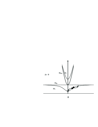
Figure 1: Polariton energy ($\omega_{\pm}$) vs incident angle at detuning $\Delta=0$ (solid). Cavity and exciton energies ($\omega_{cav}$, $\omega_{ex}$) are shown by dashed lines. Two pump polaritons (•) scatter into signal ($o)$ and idler ($\diamondsuit)$. (Adapted from Ref. 3, ).

II.1 Degenerate parametric oscillator

To start with, we consider a simplified 2-level model, where signal and idler states coincide [this model was invoked earlier to describe experiments on degenerated 4-wave mixing dfwm ]. The interaction part of the Hamiltonian for this system can be represented as

$$\mathcal{H}_{int}=V(a_{p}a_{p}a_{s}^{{\dagger}}a_{s}^{{\dagger}}+a_{s}a_{s}a_{p}^{{\dagger}}a_{p}^{{\dagger}}).$$ (3)

It is well known that quantum mechanical description of two selected states of one particle is possible in the terms of a fictitious spin 1/2 (Ref. Feynman, ). This description can be easily expanded to a system of $N$ bosons occupying two quantum-mechanical states. Let us introduce operators

$$X=\frac{1}{2}\left(a_{s}a_{p}^{{\dagger}}+a_{p}a_{s}^{{\dagger}}\right)$$ (4)

$$Y=-\frac{\mathrm{i}}{2}\left(a_{s}a_{p}^{{\dagger}}-a_{p}a_{s}^{{\dagger}}\right)$$

$$Z=\frac{1}{2}\left(a_{p}^{{\dagger}}a_{p}-a_{s}^{{\dagger}}a_{s}\right)$$

whose mean values give the difference of occupation numbers of the two states ($Z$) and second-order correlations between them ($X$ and $Y)$. These operators obey the commutation relations of angular momentum components:

$$[X,Y]=\mathrm{i}Z,\quad[Z,X]=\mathrm{i}Y,\quad[Y,Z]=\mathrm{i}X$$ (5)

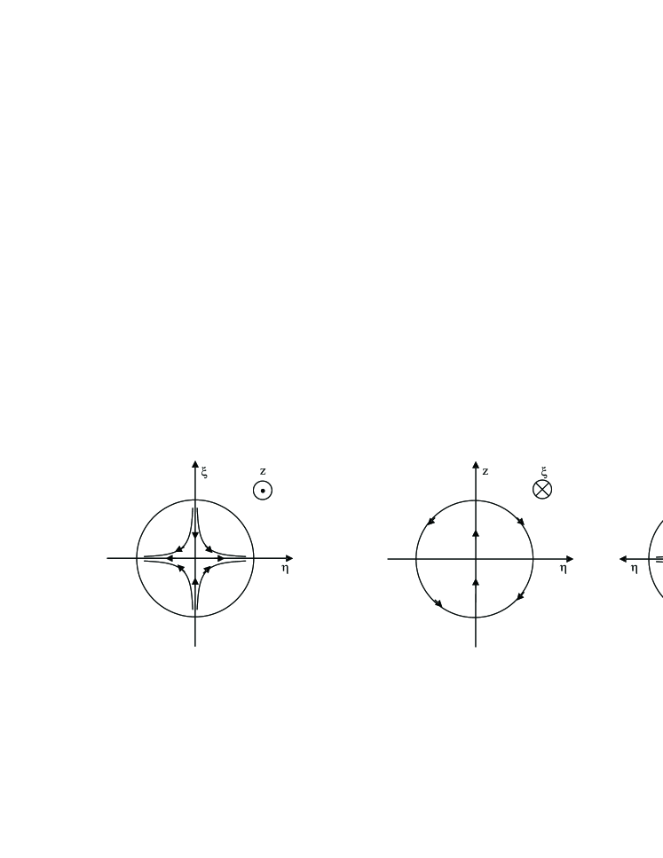
Figure 2: Schematic plots of the classically stable trajectories for the degenerate parametrical oscillator.

Therefore, we introduce a pseudospin vector $\bm{I}$ with components $X$, $Y$, $Z$ and the value $I=N$/2:

$$X^{2}+Y^{2}+Z^{2}=I(I+1)=\frac{N^{2}}{4}+\frac{N}{2},$$ (6)

where $N$ is the total number of polaritons.

For further treatment, it is more convenient to use another set of variables $\xi,\eta,Z$ where $\xi$ and $\eta$ are defined as

$$\xi=\frac{X+Y}{\sqrt{2}},\quad\eta=\frac{X-Y}{\sqrt{2}}.$$ (7)

The commutation relations for $\eta$ and $\xi$ are the same as for $X$ and $Y$ respectively because $\eta$ and $\xi$ are obtained as a result of rotation of the coordinate frame in the $(X,Y)$ plane. In terms of new variables, the interaction part of the Hamiltonian Eq. (3) can be written as

$$\mathcal{H}_{int}=2V(\xi\eta+\eta\xi)$$ (8)

Using commutation relations (Eqs. (5) and (7)) we obtain the following Heisenberg equations for $\xi,\eta$ and $Z$ (dot means time derivative)

$$\dot{Z}=-\frac{4V}{\hbar}(\eta^{2}-\xi^{2}),$$ (9)

$$\dot{\eta}=\frac{2V}{\hbar}(Z\eta+\eta Z),$$

$$\dot{\xi}=-\frac{2V}{\hbar}(Z\xi+\xi Z),$$

Since the number of polaritons is very large, $I\gg 1$ and we can treat the pseudospin as a classical vector and consider trajectories of the end of this vector on a sphere with the radius $I$ (see Fig. 2). Two meridional circles ($\eta=0$ and $\xi=0$) are the stable trajectories, i.e. any trajectory starting near one of the poles ($\eta=0,\xi=0,Z=I$ and $\eta=0,\xi=0,Z=-I$) very soon comes very close to one of these circles. The equations of motion on the meridional circles are exactly solvable. For example, for $\xi=0$ we make a substitution $Z=I\cos{\varphi}$ and $\eta=I\sin{\varphi}$ which gives a single equation for $\varphi$

$$\dot{\varphi}=\frac{4VI}{\hbar}\sin{\varphi}$$ (10)

and its solution yields

$$\varphi=2\arctan{\left[\tan{\frac{\varphi_{0}}{2}}\exp{\left(\frac{4VI}{\hbar}t\right)}\right]}$$ (11)

where $\varphi_{0}$ is determined from the initial conditions. If the initial condition corresponds to the correlated pump and signal states ($\eta$ is non-zero), then $\varphi_{0}=\arcsin{(\eta/I)}\approx\eta/I$. If signal and pump are initially not correlated, $\varphi_{0}=0$ and our approximation evidently fails because all the time derivatives in Eqs. (9) stay zero all the time. In this important case we should go beyond the classical approximation and take into account quantum fluctuations of pseudospin components 18 .

In order to do this we come back to the set of equations (9) but we will treat them as quantum equations for operators $(\xi,\eta,Z)$. Using Eq. (6) we can see that at the initial moment, when $I-|Z|\ll I$, mean square fluctuations of $\xi$ and $\eta$ are equal to $\langle\xi^{2}\rangle=\langle\eta^{2}\rangle=N/4+N/2(N/2-|Z|)$. At small $\xi$ and $\eta$, $|Z|\approx I$ and is approximately constant. We can therefore simplify Eqs. (9) by putting $Z=I$, as follows

$$\dot{\eta}=\frac{4V}{\hbar}I\eta,$$ (12)

$$\dot{\xi}=-\frac{4V}{\hbar}I\xi.$$

These equations are exactly solvable and give an exponential growth of $\eta$ and exponential decrease of $\xi$. So, at longer time delays, when the approximate Eqs. (12) are not valid, we can still put $\xi\approx 0$ and consider the motion along the corresponding classically stable trajectory, but $\xi$, $\eta$ and $Z$ should be treated as quantum-mechanical operators. The commutation relations at $\xi\rightarrow 0$ simplify:

$$[\eta,Z]=0,\quad[\xi,Z]=\mathrm{i}\eta,\quad[\eta,\xi]=\mathrm{i}Z.$$ (13)

Therefore, one can represent operators $Z$, $\eta$ and $\xi$ as $\xi=-\mathrm{i}\partial/\partial\varphi$, $Z=\rho\cos{\varphi}$, $\eta=\rho\sin{\varphi}$ where $\rho$ and $\varphi$ are classical (not operatorial) variables. In this approximation, the Hamiltonian (8) corresponds to the following time-dependent Schroedinger equation:

$$\dot{\Psi}=-\frac{2V\rho}{\hbar}\left(2\sin{\varphi}\frac{\partial\Psi}{\partial\varphi}+\Psi\cos{\varphi}\right)$$ (14)

This equation allows for explicit integration, namely

$$\Psi^{2}\sin{\varphi}=F\left(\frac{4V\rho}{\hbar}t-\ln{\left|\tan{\frac{\varphi}{2}}\right|}\right),$$ (15)

where $F$ is a function to be determined from the initial conditions. It is worth noting that $|F|d\varphi=|\Psi|^{2}dZ$ gives a probability distribution over $Z$ for the degenerate parametric oscillator.

Eq. (15) shows that in the limit of large number of polaritons, $N\gg 1$, the dynamics of our system is essentially classical and its wavefunction can be replaced by the classical probability distribution, which, in turn, satisfies the Liouville equation 19 . Actually, comparing the arguments of the function $F$ in Eq. (15) and classical solutions for $\varphi(t)$ given by Eq. (11), one can see that the probability distribution $F(\varphi,t)$ at any time moment $t$ can be obtained from the initial one, $F_{0}(\varphi_{0})$, as $F(\varphi,t)=F_{0}(\varphi(t))$, where $\varphi(t)$ is found by solving the classical system (9). In other words, one needs just to solve equations (9), treating $Z$, $\xi$, and $\eta$ as classical variables, for a set of different initial conditions with the statistics reflecting the initial $|\Psi|^{2}$, and then the probabilities for all the pseudospin components at any time can be obtained.

The validity of our approximation can be checked if we notice that on a short time-scale after an initial moment our system is equivalent to the harmonic oscillator with the inverted potential ($\mathcal{H}_{int}\propto p^{2}-x^{2}$, where $p$ and $x$ are generalized momentum and coordinate respectively). For such a problem the quasi-classical approximation is valid when the spread of the wavefunction is larger than the oscillator length (root mean square of $x$ in parabolic potential) 19 . In our case, when almost all the polaritons are initially in the pump state, the wavefunction at $t=0$ is an eigenfunction of the operator $Z$. On the other hand, this function is the first eigenfunction of the harmonic oscillator. So, initially, the width of the wavefunction is the same as the oscillator length, but in-plane components of the pseudopsin rapidly increase with time (see Eq.(12)), and the wavefunction spreads into the region of validity of the quasi-classical model. This means that the dynamics of the pseudospin is quasi-classical at any time except the short initial time range, where the system obeys analytically solvable Eqs.(12).

The above analysis refers to the first half-period of the hyperspin motion. For the second half-period the same arguments can be used with the only difference that $\eta\to 0$ serves as the momentum operator and $\xi$ becomes the classical coordinate variable.

II.2 General case

The description of the non-degenerate parametric oscillator (with different signal and idler states) is analogous to the previous case. Here, to deal with three polariton states, we introduce a 9-dimensional hyperspin pseudovector. Its components describe correlations between all pairs of states. For example, “signal-pump” components are

$$X_{1}=\frac{1}{2}\left(a_{s}a_{p}^{\dagger}+a_{p}a_{s}^{\dagger}\right)$$ (16)

$$Y_{1}=-\frac{\mathrm{i}}{2}\left(a_{s}a_{p}^{\dagger}-a_{p}a_{s}^{\dagger}\right)$$

$$Z_{1}=\frac{1}{2}\left(a_{p}^{\dagger}a_{p}-a_{s}^{\dagger}a_{s}\right)$$

The remaining components $X_{2},Y_{2},Z_{2}$ describing correlations between pump and idler and $X_{3},Y_{3},Z_{3}$ for the idler-signal correlations can be obtained by respective changing of indices. As it can be readily seen from the definition, $Z_{1}+Z_{2}+Z_{3}=0$. The commutation relations for the hyperspin components with the same index were already obtained in the previous section. Other components obey the following relations

$$[X_{\alpha},X_{\alpha+1}]=[Y_{\alpha+1},Y_{\alpha}]=\frac{\mathrm{i}}{2}Y_{\alpha-1},$$ (17)

$$[X_{\alpha},Y_{\alpha+1}]=[Y_{\alpha},X_{\alpha+1}]=\frac{\mathrm{i}}{2}X_{\alpha-1},$$

$$[X_{\alpha},Z_{\alpha+1}]=[X_{\alpha},Z_{\alpha-1}]=\frac{\mathrm{i}}{2}Y_{\alpha},$$

$$[Y_{\alpha},Z_{\alpha+1}]=[Y_{\alpha},Z_{\alpha-1}]=-\frac{\mathrm{i}}{2}X_{\alpha},$$

$$[Z_{\alpha},Z_{\alpha+1}]=0.$$

where $\alpha\in\left\{1,2,3\right\}$, $\alpha\pm 3\equiv\alpha$. The following combination plays the role of the squared total angular momentum:

$$\sum_{i}(X_{i}^{2}+Y_{i}^{2}+\frac{2}{3}Z_{i}^{2})=\frac{N^{2}}{3}+N.$$ (18)

The interaction Hamiltonian can be expressed in terms of the hyperspin operators in a very simple form

$$\mathcal{H}_{int}=2V(X_{1}X_{2}+Y_{1}Y_{2}).$$ (19)

Free propagation terms can be written as

$$\mathcal{H}_{0}=\frac{2}{3}\left[(E_{p}-E_{i})Z_{1}+(E_{i}-E_{p})Z_{2}+(E_{s}-E_{i})Z_{3}+\right.$$ (20)

$$+\left.(E_{s}+E_{p}+E_{i})\frac{N}{2}\right].$$

Our next step is to obtain a set of Heisenberg equations for the hyperspin operators. Using commutation relations (17) and simple algebra we come to

$$\dot{Z}_{1}=-\frac{{3V}}{\hbar}(X_{1}Y_{2}-Y_{1}X_{2}),\mathrm{{}}$$ (21)

$$\halign{\hbox to\displaywidth{$\hfil\displaystyle#\hfil$}\cr 0.0pt{\hfil$\displaystyle\dot{Z}_{2}=\frac{{3V}}{\hbar}(X_{1}Y_{2}-Y_{1}X_{2}),\cr 0.0pt{\hfil$\displaystyle\dot{X}_{1}=\frac{V}{\hbar}(X_{1}Y_{3}+Y_{1}X_{3}+2Z_{1}Y_{2})-\frac{{E_{p}-E_{s}}}{\hbar}Y_{1},\cr 0.0pt{\hfil$\displaystyle\dot{X}_{2}=-\frac{V}{\hbar}(X_{3}Y_{2}+Y_{3}X_{2}-2Y_{1}Z_{2})-\frac{{E_{i}-E_{p}}}{\hbar}Y_{2},\cr 0.0pt{\hfil$\displaystyle\dot{Y}_{1}=-\frac{V}{\hbar}(Y_{1}Y_{3}-X_{1}X_{3}+2Z_{1}X_{2})+\frac{{E_{p}-E_{s}}}{\hbar}X_{1},\cr 0.0pt{\hfil$\displaystyle\dot{Y}_{2}=-\frac{V}{\hbar}(X_{3}X_{2}+Y_{3}Y_{2}+2X_{1}Z_{2})+\frac{{E_{i}-E_{p}}}{\hbar}X_{2},\cr 0.0pt{\hfil$\displaystyle\dot{X}_{3}=-\frac{V}{\hbar}(X_{1}Y_{1}+Y_{1}X_{1}-X_{2}Y_{2}-Y_{2}X_{2})+\frac{{E_{i}-E_{s}}}{\hbar}Y_{3},\cr 0.0pt{\hfil$\displaystyle\dot{Y}_{3}=-\frac{V}{\hbar}(X_{1}^{2}-Y_{1}^{2}+Y_{2}^{2}-X_{2}^{2})-\frac{{E_{i}-E_{s}}}{\hbar}X_{3}.\cr}}}}}}}}$$

Further treatment of this system is very similar to one we applied in the degenerate case. The hyperspin system (21) has a classically stable trajectory defined by the following conditions:

$$Y_{2}=X_{1},\quad X_{2}=-Y_{1},\quad Y_{1}=\pm X_{1}.$$ (22)

The same argumentation as in the Sec. IIA shows that in the limit of large number of polaritons the motion of system is concentrated near this trajectory. This fact allows us to reduce number of relevant variables. In order to do it, it is convenient to use another set of variables, namely

$$\eta_{\pm}=\frac{1}{2}(X_{1}+Y_{2}\pm X_{2}\mp Y_{1}),$$ (23)

$$\xi_{\pm}=\frac{1}{2}(X_{2}+Y_{1}\pm X_{1}\mp Y_{2}),$$

$$\zeta_{\pm}=\frac{1}{2}(Z_{1}-Z_{2}\mp X_{3}).$$

On the classically stable trajectory defined by Eq.(22), $\xi_{\pm}=0$, $\eta_{\pm}=X_{1}\mp Y_{1}$ and $\zeta_{\pm}=Z_{1}\mp X_{3}/2$. These variables are remarkable by the fact that the commutation relations of the variables with the same index (+ or $-$) are the same as commutation rules for the operators of the angular momentum:

$$[\eta_{\pm},\xi_{\pm}]=\mathrm{i}\zeta_{\pm},\quad[\xi_{\pm},\zeta_{\pm}]=\mathrm{i}\eta_{\pm},\quad[\eta_{\pm},\zeta_{\pm}]=-\mathrm{i}\xi_{\pm},$$ (24)

while the commutators of variables with different indices, and of any of them with $Y_{3}$, are either exactly, or approximately equal to zero in the vicinity of the classicaly stable trajectory Eq. (22). When the hyperspin is close to the classically stable trajectory, the commutator of $\eta_{\pm}$ and $\zeta_{\pm}$ becomes negligible and the following substitution is possible

$$\zeta_{\pm}=\rho_{\pm}\cos{\varphi_{\pm}},\quad\eta_{\pm}=\rho_{\pm}\sin{\varphi_{\pm}},$$ (25)

where $\rho_{\pm}$ and $\varphi_{\pm}$ can be treated as $c$-numbers. To satisfy first two relations in Eq. (24), one should take

$$\xi_{\pm}=-\mathrm{i}\frac{\partial}{\partial\varphi_{\pm}}.$$ (26)

In terms of the new variables, the interaction Hamiltonian Eq.(2) is decomposed in two parts describing independent degenerate parametric oscillators

$$H_{int}=V\sum_{j=\pm}(\eta_{j}\xi_{j}+\xi_{j}\eta_{j})=-\mathrm{i}V\sum_{j=\pm}\rho_{j}\left(2\sin{\varphi_{j}}\frac{\partial}{\partial\varphi_{j}}+\cos{\varphi_{j}}\right).$$ (27)

Here we assume that the parametric oscillator wavefunction $\Psi$ depends on $\rho_{\pm}$ and $\varphi_{\pm}$. At the exact resonance, $E_{p}-E_{s}=E_{i}-E_{p}$ and free propagation term in the Hamiltonian may be omitted, since all possible configurations of the parametric oscillator have equal energies. The solution of the corresponding Schoedinger equation is a function of two arguments, namely

$$\Psi^{2}\sin{\varphi_{+}}\sin{\varphi_{-}}=$$ (28)

$$F\left(\frac{2V\rho_{+}}{\hbar}t-\ln{\left|\tan{\frac{\varphi_{+}}{2}}\right|},\frac{2V\rho_{-}}{\hbar}t-\ln{\left|\tan{\frac{\varphi_{-}}{2}}\right|}\right).$$

The function $F$ is determined from initial conditions in the same way as for the two-level model. The physical meaning of Eq. (28) is exactly the same as in the case of the two-level model: we can see that, for a large number of polaritons, the wavefunction can be replaced by a classical probability distribution which satisfies the Liouville theorem and evolves in accordance to the set of dynamical equations for hyperspin components (Eq.(21)).

II.3 Finite polariton lifetimes

The dynamical system considered above is idealysed as it does not include dissipation processes. In reality, polaritons have finite lifetimes dependent on the quality factor of the cavity and on the non-radiative broadening of the exciton. The decay of polaritons can be taken into account phenomenologically within the hyperspin approach, by adding linear dissipation terms to Eqs.(21), in analogy to Bloch equations. In the most general case, to keep linear dependence of the decay rate on the population of polariton states, such terms should have the following form: the total polariton population (which has been so far assumed constant) is now given by the equation $\dot{N}=-\alpha N-2\bm{\beta}\cdot\bm{I}$, where $\alpha$ and all the components of the vector $\bm{\beta}$ are constants; and the dissipation of the hyperspin vector is determined by the term $-\frac{1}{2}N\bm{\beta}-\alpha\bm{I}+\hat{\delta}\bm{I}$, where $\hat{\delta}$ is a second-rank tensor. (We remind that $\bm{I}$ is the 9-dimensional hyperspin pseudovector.) The parameters $\alpha$, $\bm{\beta}$, and $\hat{\delta}$ should be chosen in such a way as to provide given values of the inverse lifetimes $\gamma_{k}$ ($k=s,p,i$) of polaritons in signal (s), pump (p), and idler (i) states for any direction of the hyperspin. This condition is met if

$$\alpha=1/3(\gamma_{s}+\gamma_{p}+\gamma_{i}),$$ (29)

$$\beta_{Z_{1}}=1/3(\gamma_{p}-\gamma_{s}),$$

$$\beta_{Z_{2}}=1/3(\gamma_{i}-\gamma_{p}),$$

$$\beta_{Z_{3}}=1/3(\gamma_{s}-\gamma_{i}),$$

and the components of tensor $\hat{\delta}$ are

$$\delta_{Z_{1},Z_{2}}=-\delta_{Z_{3},Z_{2}}=\beta_{Z_{2}},\quad\delta_{Z_{1},Z_{3}}=-\delta_{Z_{2},Z_{3}}=-\beta_{Z_{3}},$$ (30)

$$\delta_{Z_{2},Z_{1}}=-\delta_{Z_{3},Z_{1}}=-\beta_{Z_{1}},$$

and all the other components of $\bm{\beta}$ and $\hat{\delta}$ are zero.

III NUMERICAL RESULTS AND DISCUSSION

Figure 3: Signal (solid) and pump (dashed) populations as a function of time. Idler population coincides with signal one. Main figure corresponds to the results obtained in the hyperspin formalism, and inset shows populations obtained by the direct diagonalization of the interaction hamiltonian. The difference in the behavior at time large than 7 ps may be attributed to the low ($N=100$) number of particles in our simulations.

Figure 4: Time dependence of the signal (solid) and pump (dashed) populations in the case of coherent (a) and thermal (b) pumping without lifetime. Inset shows second-order coherence for the signal state by solid line and for the pump state by dashed line.

We will focus on the situation when the pump state was initially populated while signal and idler states are empty. First of all, we will consider the pump state with a definite number of particles (Fock state). The probability distribution for $X_{i}$ and $Y_{i}$ components is given by

$$\left|\Psi(t=0)\right|^{2}=$$ (31)

$$\frac{1}{(2\pi)^{3}\sigma_{1}^{2}\sigma_{3}}\exp{\left(-\frac{X_{1}^{2}+X_{2}^{2}+Y_{1}^{2}+Y_{2}^{2}}{2\sigma_{1}}-\frac{X_{3}^{2}+Y_{3}^{2}}{2\sigma_{3}}\right)},$$

where $\sigma_{1}$ and $\sigma_{3}$ are the mean square values of the respective hyperspin components. The $Z$-projections of the hyperspin take their maximum values $Z_{1,2}=\pm N/2$, resulting in $\sigma_{3}=0$ and $\sigma_{1}=N/4$ (see Eq. (18)).

Figure 3 shows the dynamics of the signal and pump populations calculated within our hyperspin formalism compared to those obtained by direct diagonalization of the Hamiltonian Eq.(2) (see inset). The fully numerical solution of the Schoedinger equation with the Hamiltonian given by Eq. (2) has been carried out by projecting the Hamiltonian operator to the basis of the Fock states with the definite number of particles in signal, pump and idler. The eigenvalues and eigenvectors of the Hamiltonian matrix were found numerically making possible to construct a time-dependent solution in the form of a Fourier expansion. Using this time-dependent wavefunction it is possible to calculate all relevant values, namely, the average populations of states and their second order coherence (see below). Within this approach, the total number of polaritons, $N$, cannot be taken very large. We performed calculations with $N=100$, which provided reasonable computation time and, on the other hand, allowed the comparison with our quasiclassical hyperspin model valid at large $N$. Calculations within the pseudospin approach were performed by solving Eqs. (21) for a set of initial conditions distributed randomly according to Eq. (31), with a subsequent averaging. We took interaction constant $V=2.1\times 10^{-2}$ meV so as to make the product $VN\sim 2$ meV close to the realistic value 1 . Populations of signal and pump states demonstrate damped oscillations centered at $N/4$ and $N/2$ respectively. Figure 3 clearly demonstrates two main features of parametric oscillations: (a) the pump polaritons pass to signal and idler states and vice versa, and (b) polaritons arrive to the signal state with some delay with respect to the initial moment when the pump state was excited, as it was shown experimentally in Ref. 10, .

The quarter-period of the oscillations $T_{1/4}$ can be found analytically from the solution of the Schroedinger equation obtained in a previous section. For simplicity we consider an evolution of variables $\varphi_{+}$ and $\zeta_{+}$ only, assuming that the initial distributions in $+$ and $-$ variable sets are the same. According to Eq. (25), the quarter of the period corresponds to $\varphi_{+}=\pi/2$. On the other hand, if the initial value of $\varphi_{+}$ is $\varphi_{0}$, then

$$\frac{2V\rho_{+}}{\hbar}t-\ln{\left|\tan{\frac{\varphi_{+}(t)}{2}}\right|}=-\ln{\left|\tan{\frac{\varphi_{0}}{2}}\right|}.$$ (32)

(This relation can be derived comparing the argument of the function $F$ in Eq. (28) at two time moments $0$ and $t$). Thus the quarter of period at fixed $\varphi_{0}$ is given by

$$t_{1/4}=\frac{\hbar}{2V\rho_{+}}\ln{\left|\tan{\frac{\varphi_{0}}{2}}\right|}.$$ (33)

Eq. (33) should be averaged with the initial distribution of $\varphi_{0}$. Reminding that $\varphi_{0}\ll 1$, one can put $\varphi_{0}\approx\eta_{0}/\rho_{+}$ where $\eta_{0}$ is the initial value of $\eta_{+}$ and $\rho_{+}=N/2$. The variable $\eta_{+}=X_{1}-Y_{1}$ has initially Gaussian distribution with the standard deviation $\sigma_{\eta}=2\sigma_{1}=N/2$. Finally,

$$T_{1/4}=\int_{-\infty}^{\infty}\frac{1}{\sqrt{2\pi\sigma_{\eta}}}\exp{\left(-\frac{\eta^{2}}{2\sigma_{\eta}}\right)}t_{1/4}=$$ (34)

$$=\frac{\hbar}{VN}\left[\ln{\left(\frac{N}{\sqrt{2\sigma_{\eta}}}\right)}+\frac{\gamma}{2}\right]\approx 0.9\mbox{ }ps$$

where $\gamma\approx 0.577216$ is the Euler constant. This value concides with the result of numerical calculation $T_{1/4}\approx 0.9$ ps (see Fig. 3).

Figure 5: Time dependence of the signal (solid) and pump (dashed) populations in the case of coherent (a) and thermal (b) pumping with lifetime $5$ ps. Inset shows second-order coherence for the signal state by solid line and for the pump state by dashed line.

The damping of the oscillations results from the fact that the Hamiltonian (2) has almost continuous spectrum at $N\gg 1$. The summation of oscillations on different eigen-frequencies leads to the degradation and damping of the oscillations of the signal, idler and pump populations. The steady state values can be obtained from the detailed balance, i.e. the numbers of incoming and outcoming particles for each state should be equal. Since polaritons can arrive to or leave the pump state by pairs only (see Fig. 1a) and both signal and idler were not populated initially, then the steady state values for the pump, $N_{p}$, and signal, $N_{s}$, states obey the equations $N_{p}+2N_{s}=N$ and $2N_{s}=N_{p}$ with the solutions $N_{p}=N/2$ and $N_{s}=N/4$.

One can see that at time $t<7$ ps the hyperspin formalism and direct diagonalization give utterly similar results. The discrepancies at longer time delays are due to the fact that the number of particles ($N=100$) we used for simulation was too small for the quasi-classical approximation to hold on the larger time scale.

Now we proceed to discussion of quantum statistics of the parametric oscillator. We consider two different cases of initial pumping: coherent with initial pump statistics $P(N_{p})=\alpha^{2N_{p}}\exp{(-\alpha^{2})}/N_{p}!$, where $\alpha^{2}$ is the average number of particles and thermal one with initial statistics $P(N_{p})=(1-\theta)\theta^{N_{p}}$, where $\theta=\bar{N}_{p}/(1+\bar{N}_{p})$ and $\bar{N}_{p}$ is the average number of polaritons in the pump state. Figure 4 presents time dependence of the signal and pump populations and so-called second-orded coherence $g_{k}^{2}=\langle a_{k}^{{\dagger}2}a_{k}^{2}\rangle/\langle a_{k}^{{\dagger}}a_{k}\rangle^{2}$ (with $k=s,p$) which can be measured in the two-photons counting experiments. Its value characterizes the statistics of the relevant state and equals to $1$ for the coherent state and to $2$ for the thermal one. It can be seen that in the case of coherent initial pump the time dependences of the populations are similar to those obtained for the pump in the Fock state (see Fig. 4(a) and Fig. 3 for comparison). The case of thermal pumping (Fig. 4(b)) is different. The oscillations are suppressed due to the large spread of the initial distribution in the particle number and the populations of the states reach their steady values almost monotonously. Our calculations show that the steady state values of $g_{s}^{2}$ and $g_{p}^{2}$ are very close in magnitude and are $1.7$ in the case of initially coherent pump and $3.3$ for the thermal pump. These values are confirmed by the direct diagonalization of the hamiltonian ($N=100$) which gives $1.7$ and $3.2$ respectively. Such values are different from those obtained in Ref. 15, for constant wave pumping. It may seem strange that coherence dissapears in the interacting system. However this result becomes clear if one notices that in the case of the polariton laser the spontaneous coherence build-up is possible if the incoming scattering rate to the ground state is larger than the outgoing scattering rate 20 . In our case of a three level system, incoming and outgoing rates are actually the same and the coherence is destroyed by multiple scattering processes.

The calculated populations and statistics for the polaritons with finite lifetime are presented in Figure 5. The lifetimes for all states were choosen identical and equal to $\gamma^{-1}=5$ ps. One can see in the case of initially coherent pump (Fig. 5a) that the populations of signal and pump states behave nonmonotonously. From the very beginning polaritons start passing from the pump state to the signal and idler states, while initially this process goes spontaneously, and signal population growth slowly. Then, stimulated scattering switches on, and both signal and pump populations change rapidly. Then the process of return of polaritons from signal and idler to the pump state starts, etc. Because of the finite lifetime, the total number of particles in the system decreases. When it falls below the stimulation threshold $N\sim\hbar/V\gamma$ no more oscillations of the occupation numbers of signal and pump states can be seen.

The situation is different in the case of the thermal pump (see Fig. 5b): no pronounced oscillations can be seen for the pump population, however the sharp bend of the time dependence of the pump population and the increase of the signal population demonstrate that the parametric process takes place nevertheless.

Interestingly, introduction of lifetime in the system results in better coherence at $t=14$ ps $g_{s}^{2}\approx 1$ in the case of coherent pumping and in almost the same value $g_{p}^{2}\approx 3$ for the initially thermal pump.

In conclusion, we have presented the general formalism describing the dynamics of the optical parametric oscillator based on a semiconductor microcavity in the strong coupling regime in the case of large number of polaritons. The introduction of the hyperspin allows to obtain a quasi-classical solution of the quantum parametric-oscillator problem. We have shown, that the probability distribution for the hyperspin components obeys the Liouville equation. Our approach is shown to give very good agreement with the method based on the direct diagonalization of the Hamiltonian for a “moderate” number of particles ($N=100$) allowing such a numerical solution within a reasonable computation time. At the same time, our quasiclassical hypespin model radically reduces the computational complexity of the problem for large number of particles, gives a possibility to introduce finite lifetimes of polaritons, and allows to obtain some analytical results such as an expression for the period of oscillations. The presented numerical results suggest that the polariton parametric oscillator can be used as a system to grow coherence in the case where irreversible processes are present. Our formalism can be extended to allow for spin degree of freedom of polaritons and might therefore be suitable for description of polarization properties of the microcavity emission in the parametric regime.

- (1) A.V. Kavokin and G. Malpuech, Cavity polaritons, 32 volume of Thin Films and Nanostructures ed. by V.M. Agranovich and D. Taylor , Elsevier, Amsterdam (2003).
- (2) H. Deng, G. Weihs, C. Santori, J. Bloch, and Y. Yamamoto, Science 298, 199 (2002).
- (3) P.G. Savvidis, J.J. Baumberg, R. M. Stevenson, M.S. Skolnick, D.M. Whittaker, and J.S. Roberts, Phys. Rev. Lett. 84, 1547, (2000).
- (4) R.M. Stevenson, V.N. Astratov, M.S. Skolnic, D.M. Whittaker, M. Emam-Ismail, A.I. Tartakovskii, P.G. Savvidis, J.J. Baumberg, and J.S. Roberts, Phys. Rev. Lett. 84, 3680, (2000).
- (5) J.J. Baumberg, P.G. Savvidis, R.M. Stevenson, A.I. Tartakovskii, D.M. Whittaker, and J.S. Roberts, Phys. Rev. B 62, 16247, (2000).
- (6) A. I. Tartakovskii, D. N. Krizhanovskii, and V. D. Kulakovskii, Phys. Rev. B 62, 13298, (2000).
- (7) G. Messin, J. Ph. Karr, A. Baas, G. Khitrova, R. Houdré, R.P. Stanley, U. Oesterle, and E. Giacobino, Phys. Rev. Lett. 87, 127403, (2001).
- (8) A. Huynh, J. Tignon, O. Larsson, Ph. Roussignol, C. Delalande, R. André, R. Romestain, and Le Si Dang, Phys. Rev. Lett. 90, 106401, (2003).
- (9) S. Kundermann, M. Saba, C. Ciuti, T. Guillet, U. Oesterle, J. L. Staehli, and B. Deveaud, Phys. Rev. Lett. 91, 107402, (2003).
- (10) J. Erland, V. Mizeikis, W. Langbein, J.R. Jensen, and J.M. Hvam, Phys. Rev. Lett. 86, 5791 (2001).
- (11) P. G. Lagoudakis, P. G. Savvidis, J. J. Baumberg, D. M. Whittaker, P. R. Eastham, M. S. Skolnick, and J. S. Roberts, Phys. Rev. B 65, 161310, (2002).
- (12) A. Kavokin, P. G. Lagoudakis, G. Malpuech, and J. J. Baumberg, Phys. Rev. B 67, 195321, (2003).
- (13) C. Ciuti, P. Schwendimann, B. Deveaud, and A. Quattropani, Phys. Rev. B 62, 4825, (2000).
- (14) C. Ciuti, P. Schwendimann, and A. Quattropani, Phys. Rev. B 63, 041303, (2001).
- (15) P. Schwendimann, C. Ciuti, and A. Quattropani, Phys. Rev. B 68, 165324, (2003).
- (16) D.M. Whittaker, Phys. Rev. B 63, 193305, (2001).
- (17) P.R. Eastham and D.M. Whittaker, Phys. Rev. B 68, 075324, (2003).
- (18) K.V. Kavokin and I.A. Merkulov, Phys. Rev. B 55, 7371, (1997).
- (19) G. Messin, J.Ph. Karr, A. Baas, G. Khitrova, R. Houdré, R.P. Stanley, U. Oesterle, E. Giacobino, Phys. Rev. Lett. 87, 127403-1 (2001)
- (20) R.P. Feynman, F.L. Vernon, R.W. Helwarth, J. Appl. Phys. 28, 49 (1957)
- (21) L.D. Landau, E.M. Lifshits, Quantum mechanics, Pergamon Press, London, (1977).
- (22) Y.G. Rubo, F.P. Laussy, G. Malpuech, A. Kavokin, and P. Bigenwald, Phys. Rev. Lett. 91, 156403, (2003). See also F.P. Laussy, G. Malpuech, A. Kavokin, and P. Bigenwald, in press.