Models of the Pseudogap State in High – Temperature Superconductors

Abstract

We present a short review of our basic understanding of the physics of copper – oxide superconductors and formulate the list of “solved” and “unsolved” problems. The main problem remains theoretical description of the properties of the normal state, requiring clarification of the nature of the so called pseudogap state.

We review simplified models of the pseudogap state, based on the scenario of strong electron scattering by (pseudogap) fluctuations of “dielectric” (AFM, CDW) short – range order and the concept of “hot” spots (patches) on the Fermi surface. Pseudogap fluctuations are described as appropriate static Gaussian random field scattering electrons.

We derive the system of recurrence equations for the one – particle Green’s function and vertex parts, taking into account all Feynman diagrams for electron scattering by pseudogap fluctuations. Results of calculations of spectral density, density of states and optical conductivity are presented, demonstrating both pseudogap and localization effects.

We analyze the anomalies of superconducting state (both $s-$ and $d$ – wave pairing) forming on the “background” of these pseudogap fluctuations. Microscopic derivation of Ginzburg – Landau expansion allows calculations of critical temperature $T_{c}$ and other basic characteristics of a superconductor, depending on the parameters of the pseudogap. We also analyze the role of “normal” (nonmagnetic) impurity scattering. It is shown that our simplified model allows semiquantitative modelling of the typical phase diagram of superconducting cuprates.

1 Basic problems of the physics of high – temperature superconductors.

We shall start with brief review of the present day situation in the physics of high – temperature superconductors, which may be useful for the reader not involved in this field.

1.1 What is really KNOWN about copper oxides:

High – temperature superconducting (HTSC) copper oxides are intensively studied for more than 15 years now. In these years, considerable progress has been achieved in our understanding of the nature and basic physical properties of these systems, despite their complicated phase diagram, containing almost all the main phenomena studied by solid state physics (Fig. 1).

It is apparent that the number of facts are now well established and are not due to any revision in the future If we talk about superconducting state, the list of “solved” problems may be formulated as follows:

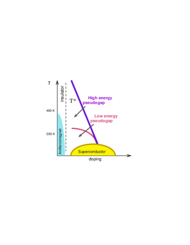
Figure 1: Typical phase diagram of copper oxide high – temperature superconductor. Different phases and anomalous regions are shown schematically. Carrier concentration, corresponding to a maximum of transition temperature $T_{c}$ is called “optimal”. Systems with lower concentrations are called “underdoped”, those with larger — “overdoped”.

• Nature of superconductivity $\rightleftharpoons$ Cooper pairing.

  It is definitely established that in these system we are dealing with

  1. $d$ – wave pairing,

     and in the spectrum of elementary excitations we observe

  2. Energy gap $\Delta\cos 2\phi$,

     where the polar angle $\phi$ determines the direction of electronic momentum in two – dimensional inverse space, corresponding to $CuO_{2}$ plane. Thus, energy gap becomes zero and changes sign on the diagonals of two – dimensional Brillouin zone.

  3. The size of pairs is relatively small: $\xi_{0}\sim 5-10a$,

     where $a$ is the lattice constant. This means that high – temperature superconductors belong to a crossover region between “large” pairs of BCS theory and “compact” Bosons picture of very strongly coupled electrons.

     Superconducting state always appears as

  4. Second order phase transition

     with more or less usual thermodynamics.

  All these facts were established during approximately first five years of studies of HTSC copper oxides. We do not give any references to original works here as the list will be to long, and quote only two review articles [1, 2].

  Situation becomes much more complicated when we consider the properties of the normal state. Almost all anomalous properties of these unusual systems appear first of all in the normal state. However, here we also can list some definitely established facts:

• Existence of the Fermi surface.

  In this sense these systems are clearly metals, though rather unusual (“bad”). Most of the data on Fermi surfaces were obtained from ARPES [3, 4], and the progress here in recent years is quite spectacular due to the great increase (more than order of magnitude!) in resolution both in energy and momentum. As an illustration of these advances in Fig. 2 we show experimentally determined Fermi surface of $La_{2-x}Sr_{x}CuO_{4}$ with $x=0.063$ [5]. Note the existence of characteristic “flat” parts of this Fermi surface. This form of the Fermi surface is rather typical for the majority of HTSC cuprates in superconducting region of the phase diagram.

  

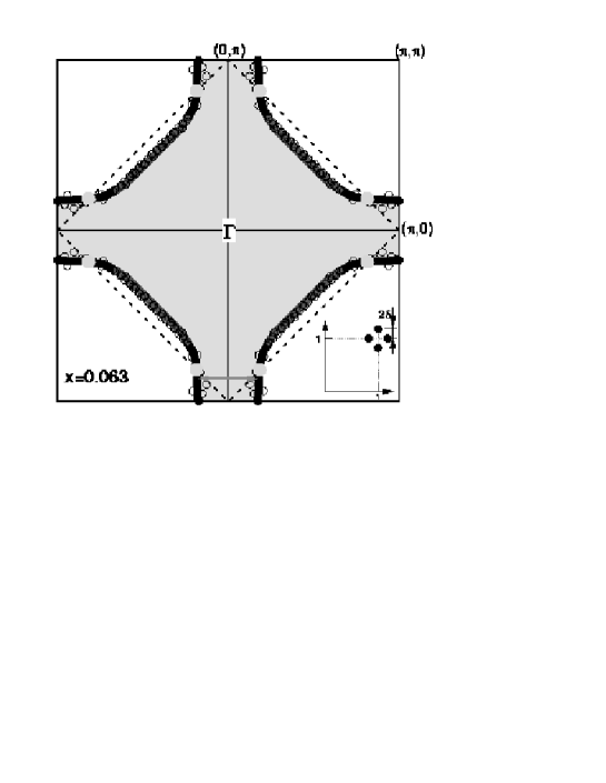
  Figure 2: Experimentally determined Fermi surface of $La_{2-x}Sr_{x}CuO_{4}$ with $x=0.063$. At the insert – schematic intensity of neutron scattering with four incommensurate peaks close to the scattering vector $(\pi,\pi)$. Dashed lines show the borders of antiferromagnetic Brillouin zone, which appear after the establishment of antiferromagnetic long – range order (period doubling). Points, where these borders intersect the Fermi surface are called “hot” spots.

• Metal — Insulator transition,

  which takes place with the change of chemical composition (as the number of carriers drops). Stochiometric $La_{2}CuO_{4}$ is an antiferromagnetic insulator (apparently of Mott type) with Neel temperature of the order of 400K. There exists well defined optical (energy) gap, and antiferromagnetism is due to the ordering of localized spins on $Cu$ ions and is well described by two – dimensional Heisenberg model. This is more or less typical also for other HTSC oxides, which thus belong to a wide class of strongly correlated electronic systems. At the same time, this dielectric state is rapidly destroyed by introduction of few percents of doping impurities. Note that the Fermi surface shown in Fig. 2, is observed, in fact, in the system which is on the edge of metal – insulator transition, which takes place at $x\sim 0.05$.

• Strong anisotropy of all properties (quasi – two – dimensional nature!).

  Current carriers (in most cases — holes) are propagating more or less freely along $CuO_{2}$ planes ($a$ and $b$ directions in orthorombic crystal), while transverse motion in orthogonal direction ($c$ axis) is strongly suppressed. Conductivity anisotropy is usually of the order of $10^{2}$ — $10^{5}$. This fact is seriously damaging from the point of view of practical applications. At the same time it is still unclear whether two – dimensionality is a necessary condition for realization of high – temperature supeconductivity.

1.2 What is still UNKNOWN about copper oxides:

Let us now list the main unsolved problems, remaining in the center of rather sharp discussions with participants sometimes not hearing each other. On the first place stays of course the

• Mechanism of Cooper pairing.

  Most researchers (not all!) do not have any doubt, that in HTSC – oxides we are dealing with Cooper pairing within more or less standard BCS “scenario”. However, the question is — what kind of interaction leads to pair formation? A number of microscopic mechanisms are under consideration:

  1. Electron – phonon [6, 7]. The main unsolved problem here is an explanation of $d$ – wave symmetry of Cooper pairing. Usually, electron – phonon coupling leads to $s$ – wave pairing. Recently there was some progress in possible ways to solve this problem [8].

  2. Spin – fluctuation [9, 10, 11, 12].

     Historically, within this approach the $d$ – wave nature of pairing in oxides was predicted. Further experimental confirmation, as well as the possibility of semiquantitative description of many properties of these systems made this approach probably most favorable (from my point of view!) among many other mechanisms.

  3. Exchange – $RVB$, $SO(5)$, …?

     These models [13, 14], as well as a number of more “exotic”, were formulated in early days of HTSC research. Enormous intellectual resources of leading theorists were and are spent on their development. However (again it is only my personal view), the completeness and “stability” of results here is incomparably less than in more traditional approaches, while real connection with experiments is relatively slight, so that all these models still remain a kind of “brain gymnastics”. Obviously, I do not deny usefulness of these models from purely theoretical point of view. For example, the discussion of symmetry connections of antiferromagnetism and superconductivity [14] is of great interest. At the same time, the most natural and useful among phenomenological approaches remains the description of superconductivity in oxides based on anisotropic version of the standard Ginzburg – Landau theory .

  At this time it is unclear, which of these mechanisms is realized or is dominant in real HTSC – oxides. And the reason for this lies in the fact, that the properties of superconducting state are relatively independent of microscopic mechanism of pairing. It is rather difficult to propose some “crucial” experiment, which will definitely confirm one of these mechanisms. In some sense, situation here is somehow similar to those existing, actually for decades, in the theory of magnetism. Since the middle of the thirties, it is well known, that the nature of magnetism is connected with exchange interaction. There exist plenty microscopic mechanisms of exchange interaction between spins (e.g. direct exchange, superexchange, $s-d$ interaction, RKKY etc.). However, it is not always possible to tell, which of these mechanisms acts in some real magnetic system. Classical example here is the problem of magnetism of iron!

• Nature of the normal state.

  Here any consensus among researchers is almost absent. Usually, recognizing the metallic nature of these systems, theorist discuss several alternative possibilities:

  1. Fermi – liquid (Landau).

  2. “Marginal” or “bad” Fermi – liquid [15].

  3. Luttinger liquid [13].

     All the talking on the possible breaking of Fermi – liquid behavior (absence of “well defined” quasiparticles) originates, from theoretical point of view, from strong electronic correlations and quasi – two – dimensionality of electronic properties of these systems, while from experimental side this is mainly due to practical impossibility of performing studies of electronic properties of the normal state at low enough temperatures (when these properties are in fact “shunted” by superconductivity, which is impossible to suppress without significant changes of the system under study). One must remember, that Fermi – liquid behavior, by definition, appears only as limiting property at low enough temperature. Thus, it is not surprising at all that it is “absent” in experiments performed at temperatures of the order of $10^{2}$K! At the same time, as we shall see below, recently there were an important experimental developments, possibly clarifying the whole problem.

  4. Disorder and local inhomogeneities.

     Practically all high – temperature superconductors are internally disordered due to chemical composition (presence of doping impurity). Thus, any understanding of their nature is impossible without the detailed studies of the role of an internal disorder in the formation of electronic properties of strongly correlated systems with low dimensionality. In particular, localization effects are quite important in these systems, and studies of these has already a long history [16]. Situation with the role of internal disorder has complicated recently with the arrival of the new data, obtained in by scanning tunneling microscopy (STM), which clearly demonstrated inhomogeneous nature of the local density of states and superconducting energy gap on microscopic scale, even in practically ideal single – crystals of copper oxides. Of many recent papers devoted to these studies, we quote only two [17, 18], where further references can be found. These results significantly modify previous ideas on microscopic phase separation, “stripes” etc. On the other hand, the presence of such inhomogeneities makes these systems a kind of “nightmare” for theorists, though the picture of inhomogeneous superconductivity due to fluctuations in the local density of states was analyzed rather long time ago [16, 19].

  5. Pseudogap.

     Now it is clear that most of the anomalies of the normal state of copper oxides is related to the formation of the so called pseudogap state. This state is realized in a wide region of the phase diagram as shown in Fig. 1, corresponding mainly to “underdoped” compositions and temperatures $T<T^{*}$. It is important to stress, that the line $T^{*}$ on Fig. 1 is rather approximate and apparently do not correspond to any phase transition and signify only a kind of crossover to the region of well developed pseudogap anomalies. In short, numerous experiments [20, 21] show that in the region of $T<T^{*}$ the systems, which are in the normal (non superconducting) state, do possess some kind of the gap – like feature in the energy spectrum. However, this is not a real gap, but some kind of precursor of its appearance in the spectrum (which is the reason for the term “pseudogap”, which appeared first in qualitative theory of amorphous and liquid semiconductors [22].). Some examples of the relevant experiments will be given below.

     Crudely speaking, the gap in the spectrum can be either of superconducting or insulating nature. Accordingly, there exist two possible theoretical “scenarios” to explain pseudogap anomalies in copper oxides. The first one anticipates formation of Cooper pairs already at temperatures higher, than the temperature of superconducting transition, with phase coherence appearing only in superconducting state at $T<T_{c}$. The second assumes, that the origin of the pseudogap state is due to fluctuations of some kind of short range order of “dielectric” type, developing in the underdoped region. Most popular here is the picture of antiferromagnetic (AFM) fluctuations, though fluctuating charge density waves (CDW) cannot be excluded, as well as structural deformations or phase separation at microscopic scales. In my opinion, most of the recent experiments provide evidence for this second scenario. So, in further discussion we shall deal only with this type of models, mainly speaking about antiferromagnetic fluctuations.

It is common view, that the final understanding of the nature of high – temperature superconductivity is impossible without clarification of the nature of the normal state. Generally speaking, we have to explain all characteristic features of the phase diagram, shown in Fig. 1. This is the main task of the theory and it is still rather far from the complete solution. In the following we shall concentrate on the discussion of some simple models of the pseudogap state and attempts to illustrate possible ways to find a solution of this main problem.

2 Basic experimental facts on the pseudogap behavior in high – temperature superconductors.

Phase diagram of Fig. 1 shows that, depending on concentration of current carriers in highly conducting $CuO_{2}$ plane, a number of phases and regions with anomalous properties can be observed in copper oxides. For small concentrations, all the known HTSC – cuprates are antiferromagnetic insulators. With the growth of carrier concentration Neel temperature $T_{N}$ rapidly drops from the values of the order of hundreds of $K$, vanishing at concentration of holes $p$ less than or of the order of $0.05$, and system becomes metallic. As concentration of holes is increasing further, the system becomes superconducting, and temperature of superconducting transition grows with the growth of carrier concentration, passing through characteristic maximum at $p_{0}\approx 0.15-0.17$ (optimal doping), and then drops and vanish at $p\approx 0.25-0.30$, though metallic behavior in this (overdoped) region remains. In the overdoped region with $p>p_{0}$ metallic properties are more or less traditional (Fermi – liquid), while for $p<p_{0}$ the system is a kind of anomalous metal, not described (in the opinion of majority of authors) by the usual theory of Fermi – liquid.

Anomalies of physical properties attributed to the pseudogap formation are observed in metallic phase for $p<p_{x}$ and temperatures $T<T^{*}$, where $T^{*}$ drops from the values of the order of $T_{N}$ at $p\sim 0.05$ vanishing at some “critical” concentration of carriers $p_{c}$, slightly greater than $p_{0}$, so that $T^{*}$ – line in Fig.1 is actually continuing under the superconducting “dome”. According to the data presented in Ref. [23] $T^{*}$ vanishes at $p=p_{c}\approx 0.19$. In the opinion of some other authors (proponents of superconducting scenario for the pseudogap) $T^{*}$ – line just passes to $T_{c}$ – line of superconducting transition somewhere close to the optimal doping $p_{0}$. In my opinion, most recent data, apparently, confirm the first variant of the phase diagram (more details can be found in Ref. [23]).

Pseudogap anomalies, in general, are interpreted as due to suppression (in this region) of the density of single – particle excitations close to the Fermi level, which corresponds to the general concept of the pseudogap [22]. The value of $T^{*}$ then determines characteristic scale of the observed anomalies and is proportional to effective energy width of the pseudogap. Let us now consider typical experimental manifestations of pseudogap behavior.

Consider first experimental data on electronic specific heat of cuprates. In metals this contribution is usually written as: $C=\gamma(T)T$, so that in the normal state ($T>T_{c}$) $\gamma\sim N(0)$, where $N(0)$ – is the density of states at the Fermi level. At $T=T_{c}$ we have the well known anomaly due to second order phase transition, so that $\gamma(T)$ demonstrates characteristic peak (discontinuity). As a typical example, in Fig. 3 we show experimental data for $Y_{0.8}Ca_{0.2}Ba_{2}Cu_{3}O_{7-\delta}$ for different values of $\delta$ [24].

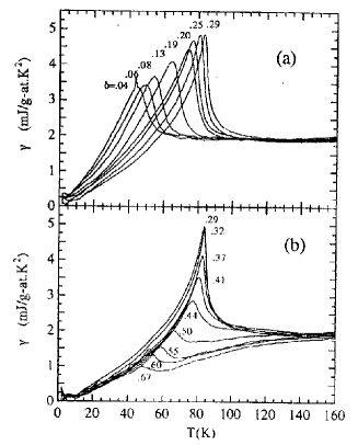
Figure 3: Coefficient $\gamma$ of electronic specific heat in overdoped (a) and underdoped (b) $Y_{0.8}Ca_{0.2}Ba_{2}Cu_{3}O_{7-\delta}$ .

We can see, that in optimally doped and overdoped samples $\gamma(T)$ is practically constant for all $T>T_{c}$, while for underdoped samples considerable drop of $\gamma(T)$ appears for $T<150-200K$. This is a direct evidence of the appropriate drop of the density of states at the Fermi level due to pseudogap formation for $T<T^{*}$.

Note also that the value of specific heat discontinuity at superconducting $T_{c}$ is significantly suppressed as we move to the underdoped region. More detailed analysis shows [23] that the drop of this discontinuity $\Delta\gamma_{c}$ actually starts at some “critical” carrier concentration $p_{c}\approx 0.19$, which is connected with the “opening” of the pseudogap.

Pseudogap formation in the density of states is clearly seen also in experiments on single particle tunneling. Thus, in highly cited Ref. [25] tunneling experiments were performed on single crystals of $Bi_{2}Sr_{2}CaCu_{2}O_{8+\delta}$ ($Bi-2212$) with different oxygen content. For underdoped samples pseudogap formation in the density of states was clearly observed at temperatures significantly higher than superconducting $T_{c}$. This pseudogap smoothly transformed into superconducting gap at $T<T_{c}$, which is often seen as an evidence of its superconducting nature. However, in Refs. [26, 27], where tunneling experiments were performed on the same system, it was directly shown, that superconducting gap exists on the “background” of the wider pseudogap and vanishes at $T=T_{c}$, while pseudogap persists at higher temperatures.

Pseudogap also shows itself in transport properties of HTSC – systems in normal state, Knight shift and NMR relaxation. In particular, changes from the usual for optimally doped linear temperature dependence of resistivity for underdoped samples and $T<T^{*}$ are often attributed to its formation. Also the value of Knight shift in such samples for $T<T^{*}$ becomes temperature dependent and drops as temperature lowers. Similar behavior is observed in underdoped samples for $(TT_{1})^{-1}$, where $T_{1}$ – is NMR relaxation time. Let us remind, that in usual metals Knight shift is just proportional to the density of states at the Fermi level $N(0)$, while $(TT_{1})^{-1}\sim N^{2}(0)$ (Korringa behavior), and resistivity $\rho$ is proportional to the scattering rate (inverse mean free time) $\gamma\sim N(0)$. Thus, significant lowering of these characteristics is naturally attributed to the drop in the density of states $N(0)$ at the Fermi level. Note that these arguments are, of course, oversimplified, particularly when we are dealing with temperature dependences. E.g. in case of resistivity this dependence is determined by inelastic scattering and physics of these processes in HTSC is still unclear. Thus, the decrease in the density of states (due to partial dielectrization of the spectrum) can also lead, in fact, to the growth of resistivity.

Pseudogap in underdoped cuprates is also observed in experiments on optical conductivity, both for electric field polarization along highly – conducting $CuO_{2}$ plane and also along orthogonal direction ($c$ – axis). These experiments are reviewed in detail in Ref. [20]. As a typical example in Fig. 4 we show the data of Ref. [28] on optical conductivity in the $CuO_{2}$ plane for different compositions of electronically conducting oxide $Nd_{2-x}Ce_{x}CuO_{4}$.

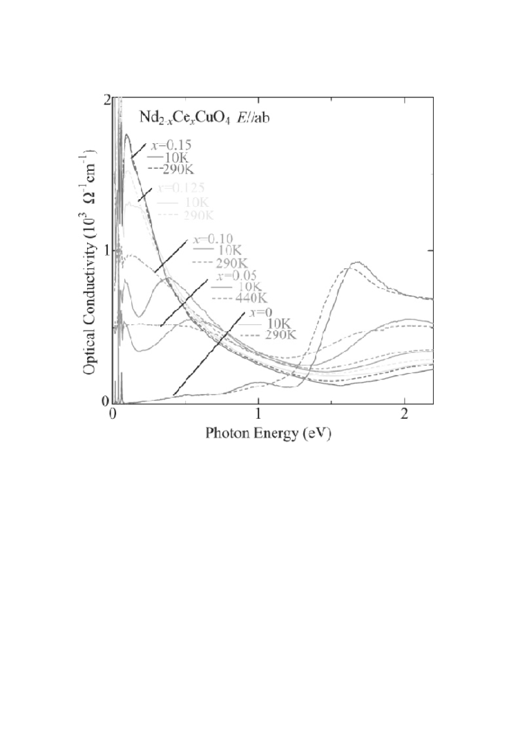
Figure 4: Real part of optical conductivity in the $ab$ – plane of $Nd_{2-x}Ce_{x}CuO_{4}$ for different temperatures and compositions $x$.

Characteristic feature here is the appearance (most clearly seen for underdoped samples with $x=0.05$ and $x=0.10$), of the shallow minimum at frequencies of the order of $0.25\ eV$ and of smooth maximum due to absorption through unusually wide pseudogap around $\omega\sim 0.5\ eV$. The nature of an additional absorption maximum seen at $\omega\sim 0.1\ eV$ can, apparently, bw attributed to localization (cf. below).

In underdoped cuprates with hole conductivity, optical conductivity is usually characterized by a narrow “Drude like” absorption peak at small frequencies, followed by a shallow minimum and smooth maximum due to pseudogap absorption through pseudogap of the order of $0.1eV$ [20, 21]. Additional peak due to localization is observed rarely, usually after the introduction of an additional disorder [29, 30, 31].

Most spectacular effects due to pseudogap formation are seen in experiments on angle resolved photoemission (ARPES). ARPES intensity (energy and momentum distribution of photoelectrons) is determined by [4]:

$$I({\bf k}\omega)=I_{0}({\bf k})f(\omega)A({\bf k}\omega)$$ (1)

where $\bf k$ – is the momentum in the Brillouin zone, $\omega$ – energy of initial state, measured with respect to the Fermi level (chemical potential), $I_{0}({\bf k})$ includes some kinematic factors and the square of the matrix elements of electron – photon interaction and in crude approximation is considered to be some constant,

$$A({\bf k},\omega)=-\frac{1}{\pi}ImG({\bf k},\omega+i\delta)$$ (2)

where $G({\bf k},\omega)$ – is Green’s function of an electron, determines the spectral density. The presence of Fermi distribution $f(\omega)=[exp(\omega/T)+1]^{-1}$ reflects the fact, that only occupied states can produce photoemission. Thus, in such a crude approximation it can be said, that ARPES experiments just measure the product $f(\omega)A({\bf k}\omega)$, and we get direct information on the spectral properties of single – particle excitations.

Consider qualitative changes in single – electron spectral density (2) due to pseudogap formation. In the standard Fermi – liquid theory, single – electron Green’ function can be written as:

$$G(\omega,{\bf k})=\frac{Z_{\bf k}}{\omega-\xi_{\bf k}-i\gamma_{\bf k}}+G_{incoh}$$ (3)

where $\xi_{\bf k}=\varepsilon_{\bf k}-\mu$ – is quasiparticle energy with respect to the Fermi level (chemical potential) $\mu$, $\gamma_{\bf k}$ – quasiparticle damping. The residue in the pole $0<Z_{\bf k}<1$, $G_{incoh}$ – is some non singular contribution due to many particle excitations. Then the spectral density is:

$$A(\omega,{\bf k})=\frac{1}{\pi}Z_{\bf k}\frac{\gamma_{\bf k}}{(\omega-\xi_{\bf k})^{2}+\gamma^{2}_{\bf k}}+...$$ (4)

where dots denote more or less smooth contribution from $G_{incoh}$, while quasiparticle spectrum determines a narrow (if damping $\gamma_{\bf k}$ is small in comparison to $\xi_{\bf k}$) Lorentzian peak. In the usual Fermi – liquid $\gamma\sim\omega^{2}\sim|{\bf k-k}_{F}|^{2}$ and quasiparticles are well defined in some (narrow enough) vicinity of the Fermi surface. In the model of “marginal” Fermi – liquid $\gamma\sim\omega\sim|{\bf k-k}_{F}|$ and quasiparticles are “marginally” defined due to $\gamma\sim\xi_{\bf k}$. In the presence of static scattering (e.g. due to impurities) a constant (independent of $\omega$) contribution $\gamma_{0}$ appears in damping.

Qualitative form of the spectral density in the Fermi – liquid picture is illustrated in Fig. 5(a).

Figure 5: Qualitative evolution of spectral density. (a) – normal metal (Fermi – liquid), $\xi_{\bf k}=0$ – at the Fermi surface. (b) – two narrow peaks, corresponding to “Bogoliubov’s” quasiparticles in a system with dielectric gap $W_{\bf k}$ (in case of long – range order of CDW or SDW type). Smooth maxima – system without long – range order (pseudogap behavior), $\xi_{\bf k}=0$ – at the Fermi surface. (c) – same as (b), but for $\xi_{\bf k}>0$, i.e. above the Fermi surface. Note characteristic asymmetry of maxima in this case.

If some long – range order (e.g. of SDW(AFM) or CDW type) appears in the system, an energy gap $W_{\bf k}$ (of dielectric nature) opens in the spectrum of elementary excitations (${\bf k}$ – dependence stresses the possibility of gap opening only on the part of the Fermi surface), and single – particle Green’s function acquires the form of Gorkov’s function (where we also add some damping $\Gamma_{\bf k}$):

$$G(\omega,{\bf k})=\frac{u^{2}_{\bf k}}{\omega-E_{\bf k}+i\Gamma_{\bf k}}+\frac{v^{2}_{\bf k}}{\omega+E_{\bf k}-i\Gamma_{\bf k}}$$ (5)

where the excitation spectrum is now:

$$E_{\bf k}=\sqrt{\xi^{2}_{\bf k}+W^{2}_{\bf k}}$$ (6)

and we introduced Bogoliubov’s coefficients:

$$u^{2}_{\bf k}=\frac{1}{2}\left(1+\frac{\xi_{\bf k}}{E_{\bf k}}\right)$$ (7)

$$v^{2}_{\bf k}=\frac{1}{2}\left(1-\frac{\xi_{\bf k}}{E_{\bf k}}\right)$$ (8)

Then the spectral density is:

$$A(\omega{\bf k})=\frac{u^{2}_{\bf k}}{\pi}\frac{\Gamma_{\bf k}}{(\omega-E_{\bf k})^{2}+\Gamma^{2}_{\bf k}}+\frac{v^{2}_{\bf k}}{\pi}\frac{\Gamma_{\bf k}}{(\omega+E_{\bf k})^{2}+\Gamma^{2}_{\bf k}}+...$$ (9)

where now appear two peaks, narrow if $\Gamma_{\bf k}$ is small enough, corresponding to “Bogoliubov’s” quasiparticles.

If there is no long – range order, but only strong scattering by fluctuations of short – range order, characterized by some correlation length $\xi$, is present in our system, it is easy to imagine, that spectral density possesses (in the same region of momentum space and energy) some precursor structure, in the form of characteristic “double – hump” structure, as it is shown qualitatively in Fig. 5. The widths of these maxima are naturally determined by parameter $v_{F}/\xi$, i.e. inverse time of flight of an electron through the region of the size of $\xi$, where “dielectric” ordering is effectively conserved. Below we shall see that rigorous analysis leads just to these results. In this sense, the further theoretical discussion will be devoted to justification of this qualitative picture.

In Fig. 6 we show ARPES data for $Bi_{2}Sr_{2}CaCu_{2}O_{8}$ [32], obtained in three different points on the Fermi surface for different temperatures.

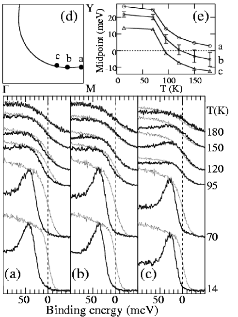
Figure 6: ARPES spectra in three different points $a,b,c$ on the Fermi surface of $Bi-2212$ for underdoped sample with $T_{c}=85K$. Thin curves — spectrum of the reference sample of $Pt$.

The presence of the gap (pseudogap) manifests itself by the shift (to the left) of the leading edge of energy distribution of photoelectrons in comparison to the reference spectrum of a good metal $(Pt)$. It is seen that this gap is closed at different temperatures for different values of ${\bf k}$, and the gap width diminishes as we move from $(0,0)-(0,\pi)$ direction in the Brillouin zone. Pseudogap is completely absent in the direction of zone diagonal $(0,0)-(\pi,\pi)$. At low temperatures this is in complete accordance with the picture of $d$ – wave pairing, which is confirmed in cuprates by many experiments [1, 2]. Important thing, however, is that this “gap” in ARPES data is observed also at temperatures significantly higher than the temperature of superconducting transition $T_{c}$.

In Fig. 7 we show angular dependence of the gap in the Brillouin zone and temperature dependence of its maximal value, obtained from ARPES [33] for several samples of $Bi-2212$ with different compositions. It is seen that the general $d$ – wave like symmetry is conserved and the gap in optimally doped sample vanishes practically at $T=T_{c}$, while for underdoped samples we observe typical “tails” in the temperature dependence of the gap for $T>T_{c}$. Qualitatively we may say that the formation of an anisotropic pseudogap at $T>T_{c}$, which smoothly transforms into superconducting gap for $T<T_{c}$, leads to “destruction” parts of the Fermi surface of underdoped samples, close to the point $(0,\pi)$ (and symmetrical to it), already for $T<T^{*}$, and the sizes of these parts grow as temperature lowers [32].

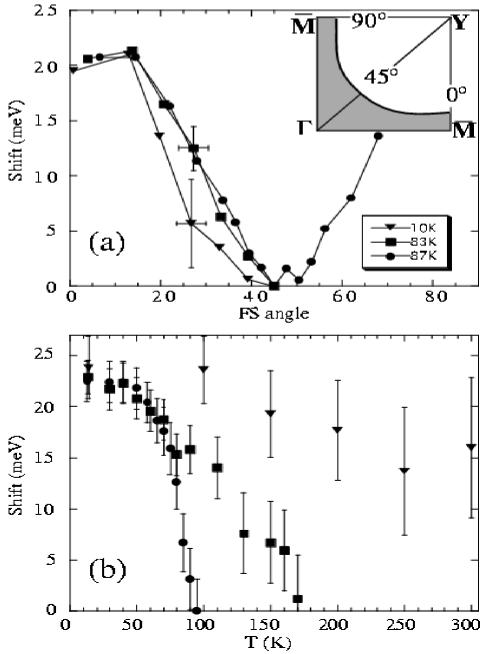
Figure 7: Angular and temperature dependences of energy gap in $Bi-2212$, obtained from ARPES data for samples with $T_{c}=87K$ (nearly optimally doped), $T_{c}=83K$ and $T_{c}=10K$ (underdoped): (a) – the value of ARPES gap, measured at different points of the Fermi surface (shown at the insert), with positions determined by polar angle, measured from the direction $\Gamma\bar{M}$, $d$ – wave symmetry of the gap is obvious. (b) – temperature dependence of the maximal gap, measured close to point $\bar{M}$.

Of central interest is, of course, the evolution of the spectral density $A({\bf k}_{F},\omega)$ at the Fermi surface. Under rather weak assumptions it can be directly determined from ARPES data [32]. Assuming electron – hole symmetry (always valid close enough to the Fermi surface, in reality for $|\omega|$ less than some tenths of $meV$) we have $A({\bf k}_{F},\omega)=A({\bf k}_{F},-\omega)$, so that taking into account $f(-\omega)=1-f(-\omega)$, from (1) and for ${\bf k}={\bf k}_{F}$ we obtain $I(\omega)+I(-\omega)=A({\bf k}_{F},\omega)$. Thus, the spectral density at the Fermi surface can be directly determined using symmetrized experimental data $I(\omega)+I(-\omega)$. As an example of such analysis, in Fig. 8 we show the dtat of Ref. [34] for underdoped sample of $Bi-2212$ with $T_{c}=83K$ and overdoped with $T_{c}=82K$ at different temperatures. It is seen that pseudogap existence clearly manifests itself in characteristic “double – humps” structure of spectral density, which appears (in an underdoped system) for temperatures significantly higher than $T_{c}$.

Figure 8: Symmetrized ARPES spectra for overdoped sample of $Bi-2212$ with $T_{c}=82K$ (a) and underdoped sample with $T_{c}=83K$ (b) at the point of intersection of the Fermi surface with the border of Brillouin zone $(0,\pi)-(\pi,\pi)$.

We see that these data completely correspond to the expected qualitative form of spectral density in the pseudogap state.

Let us stress once again, that well defined quasiparticles correspond to narrow enough peak in the spectral density $A({\bf k}_{F},\omega)$ at $\omega=0$. Such behavior, until recently, was in practically never observed in copper oxides. However, it was discovered some time ago that in superconducting phase, at $T\ll T_{c}$, there exists sharp enough peak of the spectral density, corresponding to well defined quasiparticles, in the vicinity of an intersection of the Fermi surface with diagonal of the Brillouin zone (direction $(0,0)-(\pi,\pi)$), where superconducting gap vanishes [35]. At the same time, close to the point $(0,\pi)$ the Fermi surface remains “destroyed” by both superconducting gap and the pseudogap. The studies of these “nodal” quasiparticles id of great importance and lead to some clarification of the problem of Fermi – liquid behavior. Most recent data show, that quasiparticle peak in diagonal direction persists also at temperatures much higher than $T_{c}$. This is clearly seen from the data of Ref. [36], shown in Fig. 9, where we can see the evolution of this peak as we move along the Fermi surface. It is seen that quasiparticle behavior is valid everywhere for overdoped samples and only in the vicinity of diagonal for underdoped (and optimal). Quasiparticle peak in diagonal direction persists even for strongly underdoped samples, which are on the edge of metal – insulator transition [5].

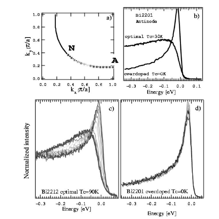
Figure 9: ARPES spectra, measured at different point at the Fermi surface, moving from the diagonal direction in Brillouin zone to $(\pi,0)$: (a) – points, where data were taken; (b) – comparison of data in “antinodal” point $A$ (vicinity of $(\pi,0)$) in optimally doped and overdoped $Bi2201$; (c) – data for optimally doped $Bi2212$ with $T_{c}=90K$, obtained at $T=140K$; (d) – similar data for overdoped $Bi2201$ with $T_{c}=0$, obtained at $T=140K$.

From data shown in Fig. 10 [36], we can also see significant anisotropy of static (or more precisely quasistatic within limits of ARPES resolution) scattering, growing as we move to the vicinity of $(0,\pi)$, which can obviously be related to pseudogap formation.

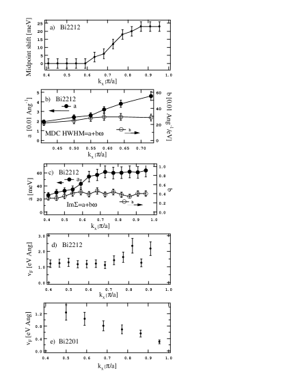
Figure 10: The fit of data on ARPES spectrum width to “marginal” dependence of the imaginary part of self – energy: $Im\Sigma=a+b\omega$. Clearly seen is anisotropy of static (quasistatic) scattering in optimally doped $Bi2212$, while dynamic (inelastic) scattering remains isotropic (c). Behavior of the velocity on the Fermi surface as shown on (d) and (e) (overdoped $Bi2201$).

Finally, in Fig. 11 we show spectacular results of Ref. [37], obtained from ARPES measurements with significantly improved resolution, from which, even by the “naked eye”, we can see that effective damping of “nodal” quasiparticles is in general (except possibly underdoped samples) more or less quadratic in energy, as we can expect for a standard Fermi – liquid. Only close to optimal doping and well into underdoped region we can see some additional contribution to scattering, most probably of magnetic nature.

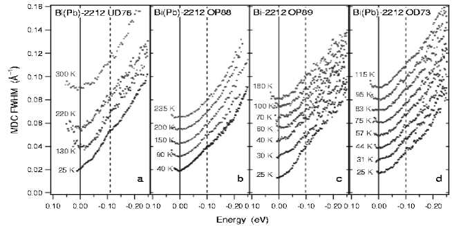
Figure 11: Experimental data on the width of ARPES peaks in $Bi(Pb)2212$ and $Bi2212$ for different temperatures, as doping level changes from underdoped sample with $T_{c}=76K$ (a) to overdoped with $T_{c}=73K$ (d).

These newest results provide quite new information on much discussed problem of Fermi – liquid behavior in HTSC – oxides. Apparently we observe typical Fermi – liquid behavior in overdoped samples, but it is “destroyed” as we move to optimal doping and into underdoped region, though only in parts of the momentum space (in the vicinity of the points like $(0,\pi)$), where pseudogap appears, leading to additional strong scattering (damping).

The growth of pseudogap anomalies as we move to the region around $(0,\pi)$, where also becomes maximal the amplitude of superconducting $d$ – wave gap, is often interpreted as an evidence of $d$ – wave symmetry of the pseudogap and of its superconducting nature, smoothly transforming into the real gap for $T<T_{c}$. However, there is lot of evidence that pseudogap actually competes with superconductivity and is, most probably, of dielectric nature. Detailed discussion of this evidence can be found e.g. in Refs. [21, 23]. Here we only limit ourselves to the most general argument — pseudogap anomalies in HTSC grow as we move deep into underdoped region, where superconductivity just vanish. It is difficult to imagine, how this type of behavior can be due to precursor Cooper pairing at $T>T_{c}$.

Of course, there are experimental data, giving direct evidence for “dielectric” nature of the pseudogap. In Fig. 12 we present ARPES data on the Fermi surface of electronic superconductor $Nd_{1.85}Ce_{0.15}CuO_{4}$ [38], which clearly show, that the “destruction” of the Fermi surface due to pseudogap formation takes place in the region around “hot spots”, appearing at intersections of the Fermi surface with borders of the “future” antiferromagnetic Brillouin zone, which would have appeared after the establishment of antiferromagnetic long – range order. Real gap in this case is obviously of the usual “band” or “insulating” nature, nothing to do with Cooper pairing of $d$ – wave symmetry. Most ARPES experiments in HTSC – oxides are performed on systems with hole – like conductivity, where the distance (in momentum space) between sides of the Fermi surface in the vicinity of $(0,\pi)$ is just smaller, than in $NdCeCuO$. Also smaller in these systems is characteristic energy scale (width) of the pseudogap, as was mentioned previously during the discussion of optical data shown in Fig. 4. Accordingly, the resolution of ARPES is apparently insufficient to resolve separate “hot spots”, which are too close to each other in the vicinity of $(0,\pi)$. In my opinion, the results of Ref. [38] practically solve the problem in favor of “dielectric” scenario of pseudogap formation in cuprates.

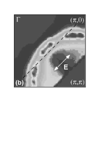
Figure 12: Fermi surface of electronic superconductor $Nd_{1.85}Ce_{0.15}CuO_{4}$ in one quadrant of the Brillouin zone, obtained by direct integration of ARPES spectra. Dashed line denotes the border of antiferromagnetic Brillouin zone.

In conclusion, we must stress that in different experiments discussed above, characteristic temperature $T^{*}$, defining crossover into the pseudogap state can somehow change, depending on the property which is being studied. However, in all cases there is some systematic dependence of $T^{*}$ on the doping level and this temperature vanishes at some concentration of carriers slightly higher than optimal.

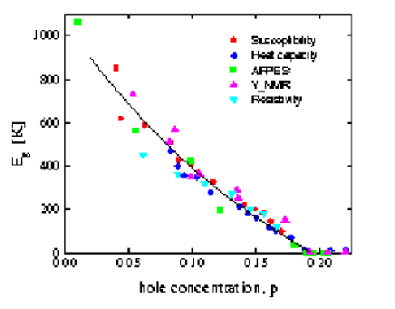
Figure 13: Dependence of the energy width of the pseudogap $E_{g}$ in $YBCO$ on hole concentration determined from different experiments.

In Fig. 13 we show a compendium of data (derived from a number of different experiments) on the energy width of the pseudogap $E_{g}$ for $YBCO$ as a function of hole concentration [23] (in this reference it was assumed, rather arbitrarily, that $E_{g}=2.5T^{*}$). It is seen that pseudogap vanishes at the critical concentration $p_{c}\approx 0.19$, slightly higher than optimal concentration of carriers, which, by the way, is an additional argument in favor of non superconducting nature of the pseudogap in cuprates.

More detailed review of miscellaneous experiments on the pseudogap formation in high temperature superconductors can be found in Refs. [20, 23].

3 Theoretical considerations – variants of simplified model.

As we mentioned above, there are two alternative scenarios to explain pseudogap anomalies in HTSC – systems. The first one is based on the model of Cooper pair formation already above the temperature of superconducting transition (precursor pairing), while the second assumes, that the origin of the pseudogap state is due to scattering by fluctuations of short – range order of “insulating” type (e.g. antiferromagnetic (SDW) or charge density wave (CDW)), existing in underdoped region of copper oxides. This second scenario seems to be more attractive, both due to a number of experimental evidences and due to a simple fact, that all pseudogap anomalies become stronger, as carrier concentration drops and the system moves farther away from optimal concentration for superconductivity towards dielectric (antiferromagnetic) phase.

Consider typical Fermi surface of electrons moving in the $CuO_{2}$ plane, shown in Fig. 2. If we neglect fine details, the observed (e.g. in ARPES) Fermi surface topology (and also the spectrum of elementary excitations) in $CuO_{2}$ plane, in the first approximation are well enough described by the usual tight – binding model:

$$\varepsilon_{\bf k}=-2t(\cos k_{x}a+\cos k_{y}a)-4t^{\prime}\cos k_{x}a\cos k_{y}a$$ (10)

where $t\approx 0.25eV$ is the nearest neighbor transfer integral, while $t^{\prime}$ is the transfer integral between second – nearest neighbors, which can change between $t^{\prime}\approx-0.45t$ for $YBa_{2}Cu_{3}O_{7-\delta}$ and $t^{\prime}\approx-0.25t$ for $La_{2-x}Sr_{x}CuO_{4}$, $a$ is the square lattice constant.

Phase transition to antiferromagnetic state induces lattice period doubling and leads to the appearance of “antiferromagnetic” Brillouin zone in inverse space as shown in Fig. 14. If the spectrum of carriers is given by (10) with $t^{\prime}=0$ and we consider the half – filled case, Fermi surface becomes just a square conciding with the borders of antiferromagnetic zone and we have a complete “nesting” — flat parts of the Fermi surface match each other after the translation by vector of antiferromagnetic ordering ${\bf Q}=(\pm\pi/a,\pm\pi/a)$. In this case and for $T=0$ the electronic spectrum is unstable, energy gap appears everywhere on the Fermi surface and the system becomes insulator, due to the formation of antiferromagnetic spin density wave (SDW). This picture corresponds to one of the popular schemes to explain antiferromagnetism in cuprates, see e.g. Ref. [39] and a review paper [40], though, as was noted above, experimental situation is well described by simple Heisenberg model with localized spins.

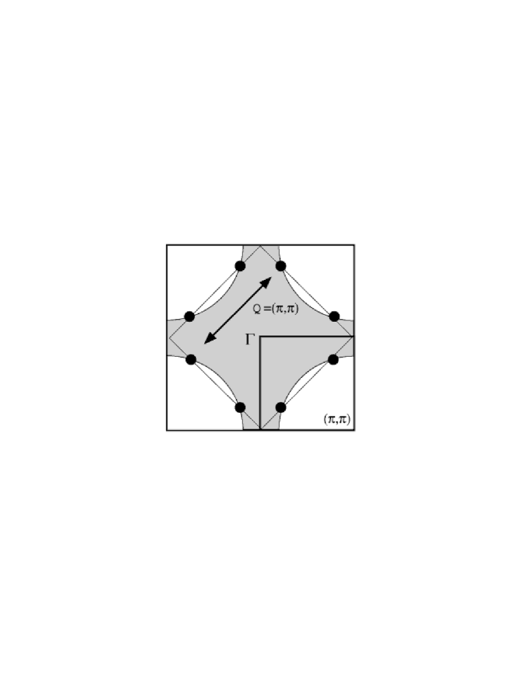
Figure 14: Fermi surface in the Brillouin zone and “hot spots” model. Magnetic zone appears in the presence of antiferromagnetic long – range order. “Hot spots” correspond to intersections of its borders with Fermi surface and are connected by the scattering vector of the order of ${\bf Q}=(\frac{\pi}{a},\frac{\pi}{a})$.

In the case of the Fermi surface shown in Fig.14 the appearance of antiferromagnetic long - range order, in accordance with general rules of the band theory, leads to the appearance of discontinuities of isoenergetic surfaces (e.g. Fermi surface) at crossing points with borders of new (magnetic) Brillouin zone due to gap opening at points connected by vector ${\bf Q}$. Note similarity of this picture with experimental data shown in Fig. 12.

In the region of cuprate phase diagram of interest to us antiferromagnetic long – range order is absent, however, a number of experiments support the existence (everywhere below the $T^{*}$ – line) of well developed fluctuations of antiferromagnetic short – range order which scatter electrons with characteristic momentum transfer of the order of ${\bf Q}$. In principle, it is not very important to consider AFM(SDW) fluctuations, similar effects may be due CDW fluctuations. There is no doubt, that such scattering processes exist (and dominate!) in cuprates in the whole pseudogap region. To convince yourself, just look at the data shown in Fig. 9!

For concreteness consider, however, the model of “nearly antiferromagnetic” Fermi – liquid [41, 42], where the effective interaction of electrons with spin fluctuations is described by dynamic spin susceptibility $\chi_{\bf q}(\omega)$, the form of which was determined by fitting to NMR experiments [43, 44]:

$$V_{eff}({\bf q},\omega)=g^{2}\chi_{\bf q}(\omega)\approx\frac{g^{2}\xi^{2}}{1+\xi^{2}({\bf q-Q})^{2}-i\frac{\omega}{\omega_{sf}}}$$ (11)

where $g$ is coupling constant, $\xi$ – correlation length of spin fluctuations, ${\bf Q}=(\pm\pi/a,\pm\pi/a)$ is vector of antiferromagnetic ordering in dielectric phase, $\omega_{sf}$ – characteristic frequency of spin fluctuations.

Dynamical spin susceptibility $\chi_{\bf q}(\omega)$ is peaked around wave vectors $(\pm\pi/a,\pm\pi/a)$, and this leads to appearance of “two types” of quasiparticles — “hot” one, with momenta in the vicinity of “hot spots” on the Fermi surface (Fig.14) and energies satisfying the inequality ($v_{F}$ – velocity at the Fermi surface):

$$|\varepsilon_{\bf k}-\varepsilon_{\bf k+Q}|<v_{F}/\xi,$$ (12)

and “cold” one with momenta close to the parts of the Fermi surface surrounding diagonals of Brillouin zone $|p_{x}|=|p_{y}|$ and not satisfying (12). This terminology is connected with strong scattering of quasiparticles in the vicinity of “hot spots” with momentum transfer of the order of ${\bf Q}$ due to interaction with spin fluctuations (11), while for quasiparticles with momenta far from “hot spots” this interaction is weak enough. In the following we shall call this “hot spots” model. Correlation length of fluctuations of short – range antiferromagnetic order $\xi$, described by (11), is an important parameter of this theory. Note that in real HTSC – systems this length is not very large, usually $2a<\xi<8a$ [45, 46].

Characteristic frequency of spin fluctuations $\omega_{sf}$, depending on the compound and doping level, is usually in the limits of $10-100K$ [45, 46], so that in most part of the pseudogap region on the phase diagram we have $2\pi T\gg\omega_{sf}$ and actually can neglect spin dynamics, limiting ourselves to quasistatic approximation:

$$V_{eff}({\bf q})=W^{2}\frac{\xi^{2}}{1+\xi^{2}({\bf q-Q})^{2}}$$ (13)

where $W$ is an effective parameter with dimensions of energy, which in the model of AFM fluctuations can be written as [47]:

$$W^{2}=g^{2}\frac{<{\bf S}_{i}^{2}>}{3}=g^{2}<(n_{i\uparrow}-n_{i\downarrow})^{2}>$$ (14)

where $g$ is interaction constant of electrons and spin fluctuations, $<{\bf S}_{i}^{2}>$ is the average square of spin on a lattice site, $n_{i\uparrow}$, $n_{i\downarrow}$ – operators of a number of electrons on a given site with appropriate spin direction. In this approximation, dynamic field of spin fluctuations is just replaced by the static Gaussian random field of “quenched” spins, antiferromagnetically correlated on lengths of the order of $\xi$.

It is clear that in the framework of our semiphenomenological approach, both correlation length $\xi$ and parameter $W$ are to be considered as some functions of carrier concentration (and temperature) to be determined from the experiment. In particular, $W$ determines the effective width of the pseudogap. Full microscopic theory of the pseudogap state is not our aim here, and in the following we shall deal only with simple modelling of appropriate transformation of electronic spectrum and its influence on different physical properties, e.g. on superconductivity.

Considerable simplification of calculations can be achieved if we substitute (13) by model interaction of the following form [48] (similar simplification was first used in Ref. [49]):

$$V_{eff}({\bf q})=W^{2}\frac{\xi^{-1}}{\xi^{-2}+(q_{x}-Q_{x})^{2}}\frac{\xi^{-1}}{\xi^{-2}+(q_{y}-Q_{y})^{2}}$$ (15)

In fact (15) is qualitatively quite similar to (13) and almost do not differ from it quantitatively in most interesting region of $|{\bf q-Q}|<\xi^{-1}$. This introduces effective one – dimensionality into our problem.

Scattering by antiferromagnetic fluctuations in HTSC – oxides is not always most intensive at commensurate vector ${\bf Q}=(\pi/a,\pi/a)$, in general case ${\bf Q}$ may correspond to incommensurate scattering (see e.g. insert at Fig. 2). Taking into account the observed topology of the Fermi surface with flat parts, as shown in Fig. 2, we can introduce another model of scattering by fluctuations of short – range order, which we call the “hot patches” model [50]. In this model we assume the Fermi surface of two – dimensional electronic system as shown in Fig. 15. The size of “hot patches” is determined by the angular parameter $\alpha$. It is well known that flat parts of the Fermi surface usually lead to instabilities towards formation of charge (CDW) or spin (SDW) density wave and formation of the appropriate long – range order and (dielectric) energy gap at these flat parts. We are interested in fluctuation region, when long – range order is not yet established.

Figure 15: Fermi surface with “hot patches”, which are shown by thick lines of the width $\sim\xi^{-1}$. The angle $\alpha$ determines the size of a “hot patch”, $\alpha=\pi/4$ corresponds to the square Fermi surface.

Fluctuations of the short – range order are again assumed to be static and Gaussian, and effective interaction is determined by (15), with scattering vectors $Q_{x}=\pm 2p_{F}$, $Q_{y}=0$ or $Q_{y}=\pm 2p_{F}$, $Q_{x}=0$. It is also assumed that fluctuations interact only with electrons from these flat (“hot”) parts of the Fermi surface, shown in Fig. 15, so that this scattering is in fact one – dimensional. In the case of $\alpha=\pi/4$ we have just a square Fermi surface and purely one – dimensional problem. For $\alpha<\pi/4$ there are also “cold” parts of the Fermi surface, where scattering is either absent or small. The choice of scattering vector ${\bf Q}=(\pm 2k_{F},0)$ or ${\bf Q}=(0,\pm 2p_{F})$ corresponds, in general, to the case of incommensurate fluctuations, as the Fermi momentum $p_{F}$ has no direct relation to the period of inverse lattice. Commensurate case can also be analyzed within this model [50].

Thus, the main idea of models under discussion reduces to the assumption of strong scattering by fluctuations of short – range order, which, according to (11), (15), is effective in a limited part of momentum space with characteristic size of the order of $\xi^{-1}$ around “hot” spots or patches, which leads to pseudogap transformation of the spectrum in these regions. It will be seen in the following, that within our assumptions these models can be solved “nearly exactly”, and much of the remaining discussion will be devoted to a description of this solution. Mostly we shall pay our attention to the discussion of the “hot spots” model as more “realistic” and not described in detail in previous reviews. As to “hot patches” model – detailed discussion and further references can be found in Ref. [21].

4 Elementary (“toy”) model of the pseudogap.

Before we go to the analysis of “realistic hot spots model” it may be useful to consider an elementary one – dimensional model of the pseudogap, which allows an exact solution in analytic form [51]. Consider an electron moving in one dimension in a random field of Gaussian fluctuations with correlation function (in momentum representation and identified with an interaction line in appropriate diagram technique) of the following form:

$$V_{eff}(Q)=2W^{2}\left\{\frac{\kappa}{(Q-2p_{F})^{2}+\kappa^{2}}+\frac{\kappa}{(Q+2p_{F})^{2}+\kappa^{2}}\right\}$$ (16)

where $\kappa=\xi^{-1}(T)$. The choice of scattering vector $Q\sim\pm 2p_{F}$, corresponds to the case of incommensurate fluctuations. An exact solution can be obtained in the asymptotic limit of $\xi\to\infty$ ($\kappa\to 0$), i.e. for very large correlation length of fluctuations of short range order. Now we can sum all Feynman diagrams of perturbation theory for an “interaction” of the form of (16), which in this limit reduces to:

$$V_{eff}(Q)=2\pi W^{2}\{\delta(Q-2p_{F})+\delta(Q+2p_{F})\}$$ (17)

Consider the simplest contribution to self – energy of an electron, described by diagram shown in Fig. 16, which we write in Matsubara representation:

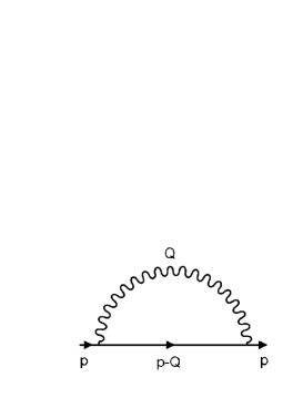
Figure 16: Simplest diagram for self – energy part of an electron. Wavy line denotes interaction $V_{eff}(Q)$.

$$\Sigma(\varepsilon_{n}p)=\int\frac{dQ}{2\pi}V_{eff}(Q)\frac{1}{i\varepsilon_{n}-\xi_{p-Q}}\approx 2W^{2}\int_{-\infty}^{\infty}\frac{dx}{2\pi}\frac{\kappa}{x^{2}+\kappa^{2}}\frac{1}{i\varepsilon_{n}+\xi_{p}-v_{F}x}=$$

$$=2W^{2}\int_{-\infty}^{\infty}\frac{dx}{2\pi}\frac{\kappa}{(x-i\kappa)(x+i\kappa)}\frac{1}{i\varepsilon_{n}+\xi_{p}-v_{F}x}=$$

$$=\frac{W^{2}}{i\varepsilon_{n}+\xi_{p}+iv_{F}\kappa}$$ (18)

where, for definiteness, we assumed $p\sim+p_{F}$, $\varepsilon_{n}>0$ and defined a new integration variable $x$ as $Q=2p_{F}+x$. We also used here “nesting” property of the spectrum $\xi_{p-2p_{F}}=-\xi_{p}$, which is always valid in one dimension for the standard $\xi_{p}=v_{F}(|p|-p_{F})$.

The limit of $\xi(T)\to\infty$ ($\kappa\to 0$) should be understood as:

$$v_{F}\kappa=v_{F}\xi^{-1}\ll Max\{2\pi T,\xi_{p}\}$$ (19)

or

$$v_{F}\kappa=v_{F}\xi^{-1}\ll 2\pi T,\qquad\xi(T)\gg|p-p_{F}|^{-1}$$ (20)

Then (18) reduces to:

$$\Sigma(\varepsilon_{n}p)\approx\frac{W^{2}}{i\varepsilon_{n}+\xi_{p}}$$ (21)

Now, for an “interaction” of the form of (17), there is no problem to write down the contribution of an arbitrary diagram of the type shown in Fig. 17. In such diagram, in the $n$ – th order in $V_{eff}(Q)$ we have $2n$ vertices, connected, in all possible ways, by interaction lines. These lines alternatively either “take away” or “bring” the momenta $Q=2p_{F}$. As a result, the appropriate analytic expression for our diagram contains alternating Green’s functions $\frac{1}{i\varepsilon_{n}-\xi_{p}}$ (entering $n$ times) and $\frac{1}{i\varepsilon_{n}+\xi_{p}}$ (also entering $n$ times) plus an extra (initial) $\frac{1}{i\varepsilon_{n}-\xi_{p}}$. Also we have to take an account of the factor $W^{2n}$. Finally, we can see, that contributions of all diagrams in a given order just coincide and their sum can be determined from pure combinatorics and is determined just by their number, which is equal to $n!$. It is obvious — there are $2n$ points (vertices) with “ingoing” or “outgoing” interaction lines. Out of these, $n$ points are connected with “outgoing” lines, which can “enter” the remaining “free” $n$ vertices in any of $n!$ ways. Use now the identity:

$$\sum_{n=0}^{\infty}n!z^{n}=\sum_{n=0}^{\infty}\int_{0}^{\infty}d\zeta e^{-\zeta}(\zeta z)^{n}=\int_{0}^{\infty}d\zeta e^{-\zeta}\frac{1}{1-\zeta z}$$ (22)

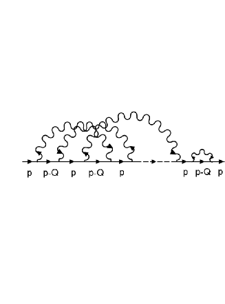
Figure 17: Diagram of an arbitrary order for the single – electron Green’s function.

Then we can easily sum the whole series for the Green’s function and obtain the following exact solution:

$$G(\varepsilon_{l}p)=\sum_{n=0}^{\infty}\frac{W^{2n}n!}{(i\varepsilon_{l}-\xi_{p})^{n}(i\varepsilon_{l}+\xi_{p})^{n}(i\varepsilon_{l}-\xi_{p})}\equiv\sum_{n=0}^{\infty}n!z^{n}(\varepsilon_{l},\xi_{p})G_{0}(\varepsilon_{l}\xi_{p})=$$

$$=\int_{0}^{\infty}d\zeta e^{-\zeta}\frac{i\varepsilon_{l}+\xi_{p}}{(i\varepsilon_{l})^{2}-\xi^{2}_{p}-\zeta W^{2}}\equiv<G_{\zeta W^{2}}(\varepsilon_{l}\xi_{p})>_{\zeta},\qquad\varepsilon_{l}=(2l+1)\pi T$$ (23)

where we have used the notation:

$$z(\varepsilon_{l},\xi_{p})=W^{2}G_{0}(\varepsilon_{l},\xi_{p})G_{0}(\varepsilon_{l},-\xi_{p})$$ (24)

Now, what has appeared is just the “normal” Green’s function of an insulator (of Peierls type):

$$G_{W^{2}}(\varepsilon_{l}p)=\frac{i\varepsilon_{l}+\xi_{p}}{(i\varepsilon_{l})^{2}-\xi^{2}_{p}-W^{2}}$$ (25)

under the “averaging” procedure of the form:

$$<...>_{\zeta}=\int_{0}^{\infty}d\zeta e^{-\zeta}...$$ (26)

It is easy to convince yourself (formal proof, as well as many other details on this model can be found in Ref. [53]) that (23) is just the Green’s function of an electron moving in an external field of the form $2V\cos(2p_{F}x+\phi)$, with amplitude “fluctuating” according to the so called Rayleigh distribution:

$${\cal P}(V)=\frac{2V}{W^{2}}e^{-\frac{V^{2}}{W^{2}}}$$ (27)

while the phase $\phi$ is distributed homogeneously on the interval from $0$ to $2\pi$.

Performing analytical continuation $i\varepsilon_{l}\to\varepsilon\pm i\delta$ from (23) we obtain (for $\varepsilon>0$):

$$ImG^{R,A}(\varepsilon\xi_{p})=\mp\pi(\varepsilon+\xi_{p})\int_{0}^{\infty}d\zeta e^{-\zeta}\delta(\varepsilon^{2}-\xi_{p}^{2}-\zeta W^{2})=$$

$$=\mp\frac{\pi}{W^{2}}(\varepsilon+\xi_{p})\theta(\varepsilon^{2}-\xi_{p}^{2})e^{-\frac{\varepsilon^{2}-\xi^{2}_{p}}{W^{2}}}$$ (28)

so that the spectral density

$$A(\varepsilon\xi_{p})=-\frac{1}{\pi}ImG^{R}(\varepsilon\xi_{p})$$ (29)

has “non Fermi – liquid like ” form, shown in Fig. 18.

Figure 18: Spectral density in the model of pseudogap state: (1)—$\xi_{p}=0$; (2)—$\xi_{p}=0.1W$; (3)—$\xi_{p}=0.5W$.

Figure 19: Density of states with pseudogap.

Let us stress, that our Green’s function does not have any poles on the real axis of $\varepsilon$, which may correspond to quasiparticle energies as required in Fermi – liquid theory.

Electronic density of states has the following form:

$$\frac{N(\varepsilon)}{N_{0}(E_{F})}=\left|\frac{\varepsilon}{W}\right|\int_{0}^{\frac{\varepsilon^{2}}{W^{2}}}d\zeta\frac{e^{-\zeta}}{\sqrt{\frac{\varepsilon^{2}}{W^{2}}-\zeta}}=2\left|\frac{\varepsilon}{W}\right|\exp\left(-\frac{\varepsilon^{2}}{W^{2}}\right)Erfi\left(\frac{\varepsilon}{W}\right)=$$

$$=\left\{\begin{array}[]{l}1\qquad\mbox{ }\qquad|\varepsilon|\to\infty\\ \frac{2\varepsilon^{2}}{W^{2}}\qquad\mbox{ }\qquad|\varepsilon|\to 0\end{array}\right.$$ (32)

where $N_{0}(E_{F})$ is the density of states of free electrons at the Fermi level, and $Erfi(x)=\int_{0}^{x}dxe^{x^{2}}$ is error function of imaginary argument. Characteristic form of this density of states is shown in Fig. 19 and demonstrate the presence of a “soft” pseudogap around the Fermi level. Obviously, this is just the density of states of one – dimensional insulator with the energy gap $2V$, averaged over fluctuations of this gap with probability distribution (27).

Remarkable property of this model is the possibility of obtaining an exact solution (sum all diagrams) also for the response function to an external electromagnetic field [51, 53]. The arbitrary diagram for the vertex part, describing the response to an external field, can be obtained from an arbitrary diagram for the Green’s function (of the type shown in Fig. 17) by an “insertion” of an external field line into any of electronic lines, as shown in Fig. 20.

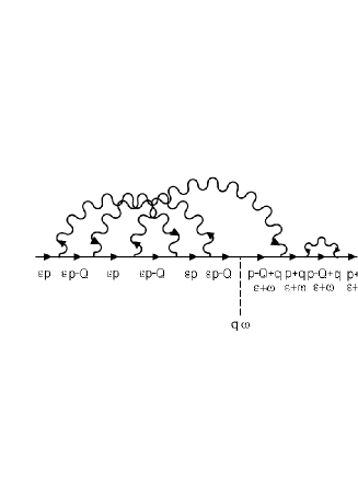
Figure 20: Diagram of an arbitrary order for the vertex part of an interaction with an external electromagnetic field.

Making such “insertions” into all diagrams of the series (23) it is possible (after some long, but direct calculations) to sum the whole series for the vertwx part and obtain closed expression for response functions, e.g. for polarization operator. Details can be found in Refs. [51, 53]). However, the structure of an answer is clear without any calculations — you must just calculate the response of an insulator with fixed gap $2V$ and afterwards average the result over gap fluctuations with distribution function (27). In particular, for polarization operator we obtain the following elegant expression $(\omega_{m}=2\pi mT)$:

$$\Pi({\bf q}\omega_{m})=\int_{0}^{\infty}d\zeta e^{-\zeta}2T\sum_{n}\int_{-\infty}^{\infty}\frac{dp}{2\pi}\left\{G_{\zeta W^{2}}(\varepsilon_{n}{\bf p})G_{\zeta W^{2}}(\varepsilon_{n}+\omega_{m}{\bf p+q})\right.+$$

$$\left.+F_{\zeta W^{2}}(\varepsilon_{n}{\bf p})F^{+}_{\zeta W^{2}}(\varepsilon_{n}+\omega_{m}{\bf p+q})\right\}=<\Pi_{\zeta W^{2}}({\bf q}\omega_{m})>_{\zeta}$$ (33)

where automatically appears the product of two “anomalous” Green’s functions:

$$F(\varepsilon_{n}p)=\frac{W^{*}}{(i\varepsilon_{n})^{2}-\xi_{p}^{2}-|W|^{2}},\quad F^{+}(\varepsilon_{n}+\omega_{m}p)=\frac{W}{(i\varepsilon_{n}+i\omega_{m})^{2}-\xi_{p}^{2}-|W|^{2}}$$ (34)

describing Umklapp processes in a system with long – range order [53]. Due to the absence of any long – range order in our model, the value of (34) vanishes after averaging over phase, while the average of pair of these functions in two – particle response (33) is non zero. Finally, under the averaging procedure over the gap fluctuations we have simply the polarization operator of an insulator (of Peierls type).

The real part of conductivity for such one – dimensional insulator with fixed gap $2W$ has the following form [53]:

$$Re\sigma_{W^{2}}(\omega)=\left\{\begin{array}[]{l}\frac{ne^{2}}{m\omega}\frac{\pi}{\sqrt{\frac{\omega^{2}}{4W^{2}}-1}}\frac{W}{\omega}\quad\mbox{ }\quad|\omega|>2W\\ 0\qquad\mbox{ }\qquad|\omega|<2W\end{array}\right.$$ (35)

It is seen, that absorption of electromagnetic energy is going through quasiparticle excitation via the energy gap and is non zero for $\omega>2W$. In the pseudogap state this expression must be averaged over fluctuations of $W$, described by distribution function (26) or (27). So finally, from (35) we get:

$$Re\sigma(\omega)=\frac{\omega_{p}^{2}}{4}\frac{W}{\omega^{2}}\int_{0}^{\frac{\omega^{2}}{4W^{2}}}d\zeta e^{-\zeta}\frac{\zeta}{\sqrt{\frac{\omega^{2}}{4W^{2}}-\zeta}}$$ (36)

Appropriate frequency dependence id shown in Fig. 21.

Figure 21: Frequency dependence of the real part of conductivity in the pseudogap state. Conductivity is given in units of $\frac{\omega_{p}^{2}}{4\pi W}$.

We can see characteristic smooth maximum of absorption through the pseudogap.

This elementary model of the pseudogap state is very useful for an analysis of a number of problems. It is easily generalized to two – dimensional case for the “hot patches” model [50]. This allows the analysis of the problem of formation of superconducting state on the “background” of this (dielectric) pseudogap [50, 54, 55, 59, 56]. In particular, due to the possibility of obtaining an exact solution in closed analytic form, it is possible to study rather fine problems of the absence of self – averaging property of superconducting order parameter in the random field of pseudogap fluctuations [54], showing the possible mechanism of formation of local inhomogeneities (“superconducting drops”) at temperatures higher than the mean – field critical temperature of superconducting transition. This may help to explain e.g. experimentally observed manifestations of superconductivity at these high temperatures (like anomalous Nernst effect), which are usually interpreted in the spirit of superconducting scenario of pseudogap formation. Possible direct connection with the picture of inhomogeneous superconductivity, observed in STM experiments [17, 18], is also obvious.

However, advantages of the model determine also its deficiencies. In particular, absolutely unrealistic is asymptotics of infinite correlation length of pseudogap fluctuations. In real systems, as was noted above, this correlation length is usually not larger than few interatomic spacings. Besides that, the growth of correlation length inevitably leads to the breaking of our assumption of the Gaussian nature of pseudogap fluctuations. Analysis of effects of finiteness of correlation length is actually a complicated problem. For one – dimensional model such generalization of the model under discussion was proposed in Ref. [57]. It was shown, that as correlation length $\xi$ becomes smaller, it leads to smooth “filling” of the pseudogap, due to the growth of the scattering parameter $v_{F}/\xi$, i.e. of the inverse time of flight of an electron through the region of the size of $\sim\xi$, where effectively we have “dielectric” ordering. The method used in Ref. [57] forms the basis of appropriate generalization to two dimensions [48, 47], which will be discussed below during our analysis of “hot spots” model. Let us also mention the simplified version of one – dimensional model with finite correlation length, similar in spirit to the model of Ref. [51, 57], proposed in Ref. [58] and used in Ref. [59] to analyze the problems of self – averaging properties of superconducting order parameter in the “hot patches” model.

5 “Hot spots” model.

5.1 “Nearly exact” solution for one – particle Green’s function.

Let us now describe our “nearly exact” solution for “hot spots” model. Consider first – order (in $V_{eff}$ (15)) contribution to electron self – energy, corresponding to simplest diagram, shown in Fig. 16:

$$\Sigma(\varepsilon_{n}{\bf p})=\sum_{\bf q}V_{eff}({\bf q})\frac{1}{i\varepsilon_{n}-\xi_{\bf p+q}}$$ (37)

For large enough correlation lengths $\xi$, the main contribution to the sum over ${\bf q}$ comes from the vicinity of ${\bf Q}=(\pi/a,\pi/a)$. Then we can write:

$$\xi_{\bf p+q}=\xi_{\bf p+Q+k}\approx\xi_{\bf p+Q}+{\bf v_{\bf p+Q}k}$$ (38)

where ${\bf v}_{\bf p+Q}=\frac{\partial\xi_{\bf p+Q}}{\partial{\bf p}}$ is the appropriate velocity of a quasiparticle on the Fermi surface. Then (37) is easily calculated and we get:

$$\Sigma(\varepsilon_{n}{\bf p})=\frac{W^{2}}{i\varepsilon_{n}-\xi_{\bf p+Q}+i(|v^{x}_{\bf p+Q}|+|v^{y}_{\bf p+Q}|)\kappa sign\varepsilon_{n}}$$ (39)

where $\kappa=\xi^{-1}$. Let us stress that both here and below “linearization” of the quasiparticle spectrum (38) under the integral (37) is performed only over small, due to large enough $\xi$, correction (of the order of $v_{F}\xi^{-1}$) to the spectrum close to the Fermi surface, while the forms of the spectrum itself $\xi_{\bf p}$ and $\xi_{\bf p+Q}$ are given by the general expression (10) with $\xi_{\bf p}=\varepsilon_{\bf p}-\mu$.

Consider now correction of the second order, shown in Fig. 22.

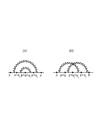
Figure 22: Diagrams of second order in effective interaction with pseudogap fluctuations.

Using (15) we obtain:

$$\Sigma(a)=\Delta^{4}\int\frac{d{\bf k_{1}}}{\pi^{2}}\int\frac{d\bf k_{2}}{\pi^{2}}\frac{\kappa}{\kappa^{2}+k_{1x}^{2}}\frac{\kappa}{\kappa^{2}+k_{1y}^{2}}\frac{\kappa}{\kappa^{2}+k_{2x}^{2}}\frac{\kappa}{\kappa^{2}+k_{2y}^{2}}$$

$$\frac{1}{i\varepsilon_{n}-\xi_{\bf p+Q}-v^{x}_{\bf p+Q}k_{1x}-v^{y}_{\bf p+Q}k_{1y}}\frac{1}{i\varepsilon_{n}-\xi_{\bf p}-v^{x}_{\bf p}(k_{1x}+k_{2x})-v^{y}_{\bf p}(k_{1y}+k_{2y})}$$

$$\frac{1}{i\varepsilon_{n}-\xi_{\bf p+Q}-v^{x}_{\bf p+Q}k_{1x}-v^{y}_{\bf p+Q}k_{1y}}$$ (40)

$$\Sigma(b)=\Delta^{4}\int\frac{d{\bf k_{1}}}{\pi^{2}}\int\frac{d\bf k_{2}}{\pi^{2}}\frac{\kappa}{\kappa^{2}+k_{1x}^{2}}\frac{\kappa}{\kappa^{2}+k_{1y}^{2}}\frac{\kappa}{\kappa^{2}+k_{2x}^{2}}\frac{\kappa}{\kappa^{2}+k_{2y}^{2}}$$

$$\frac{1}{i\varepsilon_{n}-\xi_{\bf p+Q}-v^{x}_{\bf p+Q}k_{1x}-v^{y}_{\bf p+Q}k_{1y}}\frac{1}{i\varepsilon_{n}-\xi_{\bf p}-v^{x}_{\bf p}(k_{1x}+k_{2x})-v^{y}_{\bf p}(k_{1y}+k_{2y})}$$

$$\frac{1}{i\varepsilon_{n}-\xi_{\bf p+Q}-v^{x}_{\bf p+Q}k_{2x}-v^{y}_{\bf p+Q}k_{2y}}$$ (41)

where we have used the explicit form of the spectrum (10), from which it follows, in particular, that $\xi_{\bf p+2Q}=\xi_{\bf p}$, ${\bf v}_{\bf p+2Q}={\bf v}_{\bf p}$ for ${\bf Q}=(\pi/a,\pi/a)$. If the signs of $v_{\bf p}^{x}$ and $v_{\bf p+Q}^{x}$, as well as of $v_{\bf p}^{y}$ and $v_{\bf p+Q}^{y}$ coincide, the integrals in (40) and (41) are completely determined by contributions from the poles of Lorentzians, which describe interaction with fluctuations of short – range order, so that after elementary contour integration we get:

$$\Sigma(a)=\Sigma(b)=\frac{1}{[i\varepsilon_{n}-\xi_{\bf p+Q}+i(|v_{\bf p+Q}^{x}|+|v_{\bf p+Q}^{y}|)\kappa]^{2}}\frac{1}{i\varepsilon_{n}-\xi_{\bf p}+i2(|v_{\bf p}^{x}|+|v_{\bf p}^{y}|)\kappa}$$ (42)

Here and in the following, for definiteness, we assume $\varepsilon_{n}>0$.

It is not difficult to convince yourself, that in case of coinciding signs of velocity projections at “hot spots”, similar calculation is valid for an arbitrary diagram of higher order.

Thus, in case of coinciding signs of velocity projections at the Fermi surface $v^{x}_{\bf p}$ and $v^{x}_{\bf p+Q}$, and those of $v^{y}_{\bf p}$ and $v^{y}_{\bf p+Q}$, Feynman integrals in any diagram of arbitrary order are determined only by contributions form the poles of Lorentzians in (15) and are easily calculated. Similar situation holds also in the case of velocities at “hot spots”, connected by vector ${\bf Q}$, are perpendicular to each other. In this case the contribution of an arbitrary diagram of $N$ – th order in (15) for electron self – energy has the following form:

$$\Sigma^{(N)}(\varepsilon_{n}{\bf p})=W^{2N}\prod_{j=1}^{2N-1}\frac{1}{i\varepsilon_{n}-\xi_{j}({\bf p})+in_{j}v_{j}\kappa}$$ (43)

where $\xi_{j}({\bf p})=\xi_{\bf p+Q}$ and $v_{j}=|v_{\bf p+Q}^{x}|+|v_{\bf p+Q}^{y}|$ for odd $j$ and $\xi_{j}({\bf p})=\xi_{\bf p}$ and $v_{j}=|v_{\bf p}^{x}|+|v_{\bf p}^{y}|$ for even $j$. Here $n_{j}$ is the number of interaction lines, surrounding $j$ – th Green’s function (counting from the first one in diagram) and we again take $\varepsilon_{n}>0$.

In Ref. [48] we have studied in detail when these conditions on velocity projections are satisfied in the points of the Fermi surface connected by vector ${\bf Q}$ (“hot spots”) and have presented explicit examples of appropriate geometries of the fermi surface, which can be realized for specific relations between parameters $t$ and $t^{\prime}$ in (10). In these cases expression (43) is exact, with only limitation being related to our use of “linearization” (38). In all other cases (for other relations between $t$ and $t^{\prime}$) we use (43) as rather successful Ansatz for the contribution of an arbitrary order, obtained by simple continuation of spectrum parameters $t$ and $t^{\prime}$ to the region of interest to us. Even in most inappropriate one – dimensional case [57], corresponding to square Fermi surface, appearing for (10) if $t^{\prime}=0$ and $\mu=0$, the use of this Ansatz produces results (e.g. for the density of state) which are very close quantitatively [60] to the results of an exact numerical simulation of this problem [61].

Generally speaking, note that in standard diagrammatic approaches we usually perform summation some subseries of diagrams, which are considered as dominant over some smallness parameter. Here we are dealing with much more rare situation — we can sum the whole diagram series, though contribution of each diagram is calculated probably approximately. It is in this sense that we use the term “nearly exact” solution.

Using Ansatz (43) we can see, that the contribution of an arbitrary diagram with intersecting interaction lines is actually equal to the contribution of some diagram of the same order without intersections of these lines [57]. Thus, in fact we can limit ourselves to consideration of only diagrams without intersecting interaction lines, taking the contribution of diagrams with intersections into account with the help of additional combinatorial factors, which are attributed to “initial” vertices or just interaction lines [57]. As a result we obtain the following recursion relation (continuous fraction representation [57]), which gives an effective algorithm for numerical computations [48]:

$$G_{k}(\varepsilon_{n}\xi_{\bf p})=\frac{1}{i\varepsilon_{n}-\xi_{k}({\bf p})+ikv_{k}\kappa-\Sigma_{k+1}(\varepsilon_{n}\xi_{\bf p})}\equiv$$

$$\equiv\left\{G^{-1}_{0k}(\varepsilon_{n}\xi_{\bf p})-\Sigma_{k+1}(\varepsilon_{n}\xi_{\bf p})\right\}^{-1}$$ (44)

$$\Sigma_{k}(\varepsilon_{n}\xi_{\bf p})=W^{2}\frac{v(k)}{i\varepsilon_{n}-\xi_{k}({\bf p})+ikv_{k}\kappa-\Sigma_{k+1}(\varepsilon_{n}\xi_{\bf p})}$$ (45)

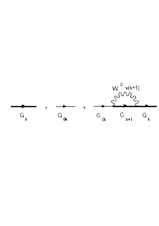
Figure 23: Graphical representation of recursion relation for the single – particle Green’s function.

Graphically this recursion relation for the Green’s function is shown in Fig. 23. The “physical” Green’s function is obtained as: $G(\varepsilon_{n}\xi_{\bf p})=G_{k=0}(\varepsilon_{n}\xi_{\bf p})$. In (44) we also defined:

$$G_{0k}(\varepsilon_{n}\xi_{\bf p})=\frac{1}{i\varepsilon_{n}-\xi_{k}({\bf p})+ikv_{k}\kappa}$$ (46)

Combinatorial factor:

$$v(k)=k$$ (47)

for the case of commensurate fluctuations with ${\bf Q}=(\pi/a,\pi/a)$ [57], if we don not take into spin structure od interaction (CDW – type fluctuations). For incommensurate CDW fluctuations [57]:

$$v(k)=\left\{\begin{array}[]{cc}\frac{k+1}{2}&\mbox{for odd $k$}\\ \frac{k}{2}&\mbox{for even $k$}\end{array}\right.$$ (48)

If we take into account (Heisenberg) spin structure of interaction with pseudogap fluctuations in “nearly antiferromagnetic Fermi – liquid” (spin – fermion model [47]), combinatorics of diagrams becomes more complicated. Thus, spin – conserving scattering processes obey commensurate combinatorics, while spin – flip scattering is described by diagrams of incommensurate case (“charged” random field in terms of Ref. [47]). In this model recursion relation for the Green’s function again is given by (45), but combinatorial factor $v(k)$ takes now the following form [47]:

$$v(k)=\left\{\begin{array}[]{cc}\frac{k+2}{3}&\mbox{for odd $k$}\\ \frac{k}{3}&\mbox{for even $k$}\end{array}\right.$$ (49)

The obtained solution for the single – particle Green’s function is asymptotically exact in the limit of $\xi\to\infty$, when solution can be found also in analytical form [51, 47]. It is also exact in trivial limit of $\xi\to 0$, when for fixed values of $W$ interaction (15) just vanishes. For all intermediate values of $\xi$ our solution gives, as already noted, very good interpolation, being practically exact for certain geometries of the Fermi surface, appearing for certain relations between parameters of the spectrum (10) [48]. Note also that our formalism can be easily used also to describe pseudogap within superconducting scenario [48, 62]. Our preference for “dielectric” scenario is based mainly on physical considerations.

Using (44) we can easily perform numerical calculations of single – electron spectral density:

$$A(E{\bf p})=-\frac{1}{\pi}ImG^{R}(E{\bf p})$$ (50)

which can also be determined from ARPES experiments [21]. In (50) $G^{R}(E{\bf p})$ represents retarded Green’s function obtained by the usual analytic continuation of (44) from Matsubara frequencies to the real axis of $E$. Analogously we cam compute single – particle density of states as:

$$N(E)=\sum_{\bf p}A(E{\bf p})=-\frac{1}{\pi}\sum_{\bf p}ImG^{R}(E{\bf p})$$ (51)

Details of these calculations and discussion of the results for our two – dimensional model can be found in Refs. [47, 48]. Here we shall demonstrate only few most important results.

As a typical example in Fig. 24 we show the results [48] for spectral density of electrons for the incommensurate (CDW) case.

Figure 24: Spectral density in the “hot spots” model, the case of incommensurate fluctuations, $\kappa a=0.01$: (1) – at the “hot spot” $p_{x}a/\pi=0.142,p_{y}a/\pi=0.587$, (2) – close to “hot spot” at $p_{x}a/\pi=0.145,p_{y}a/\pi=0.843$, (3) – far from “hot spot” at $p_{x}a/\pi=p_{y}/\pi=0.375$.

We can see that spectral density close to the “hot spot” has an expected non Fermi – liquid like form and there are no well defined quasiparticle peaks. Far from the “hot spot” spectral density is characterized by a narrow peak, corresponding to well defined quasiparticles (Fermi – liquid). In Fig. 25 from Ref. [47] we show the product of the Fermi distribution and spectral density at different points of the “renormalized” Fermi surface, defined by the equation $\varepsilon_{\bf p}-Re\Sigma(E=0{\bf p})=0$, where the “bare” spectrum $\varepsilon_{\bf p}$ is given by (10) with $t=-0.25eV,t^{\prime}=-0.35t$ and for hole concentration $n_{h}=0.16$, with coupling constant in (11) $g=0.8eV$ and correlation length $\xi=3a$ (commensurate case, spin – fermion model). We can clearly see complete qualitative agreement with ARPES data discussed above with quite different behavior close and far from the “hot spot”.

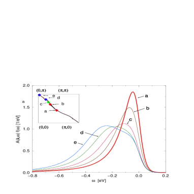
Figure 25: The product of spectral density and Fermi distribution function at different points on the Fermi surface, shown at the insert. Spin – fermion model, correlation length $\xi=3a$.

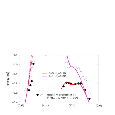
Figure 26: Positions of the maximum of the spectral density for different values of correlation length $\xi$ and hole concentrations, calculated for spin – fermion model and compared with ARPES data for $Bi_{2}Sr_{2}Ca_{1-x}Dy_{x}Cu_{2}O_{8+\delta}$ with $x=1$ (triangles) and $x=0.175$ (diamonds).

Finally, in Fig. 26 taken from Ref. [47] we show calculated (for spin fermion – model) positions of the maximum of $A(\omega{\bf k})$ for two different concentrations of holes compared with appropriate experimental ARPES data of Ref. [63] for $Bi_{2}Sr_{2}Ca_{1-x}Dy_{x}Cu_{2}O_{8+\delta}$. The point is, that positions of the maxima of spectral density in the plane of $(\omega,{\bf k})$, determined from ARPES, in an ideal system of the Fermi – liquid type define dispersion (spectrum) of quasiparticles (cf. Fig. 5(a)). For overdoped system the values of $n_{h}=0.22$ and $\xi=a$ were assumed during these calculations. The results obtained demonstrate rather well defined dispersion curves both along the diagonal of Brillouin zone, and in the direction $(0,0)-(\pi,0)$. For underdoped system it was assumed that $n_{h}=0.16$ and $\xi=3a$. In this case, in diagonal direction we again see spectral curve crossing the Fermi level, while close to “hot spots” (in the vicinity of $(\pi,0)$) there is seen only a smeared maximum of spectral density remaining approximately $200\ meV$ below the Fermi level (pseudogap). In general, agreement between theory and experiment is rather satisfactory.

Ley us now consider the single – electron density of states, defined by the integral of the spectral density $A(E{\bf p})$ over the whole Brillouin zone. Detailed calculations of the density of states in “hot spots” model were performed in Ref. [48]. As an example, in Fig. 27 we show appropriate data for the Fermi surface topology typical for HTSC – systems.

Figure 27: Single – electron density of states (in units of $1/ta^{2}$) for for different combinatorics of diagrams and $t^{\prime}/t=-0.4$, $\mu/t=-1.3$, which is typical for HTSC – cuprates: (1) — incommensurate case, (2) — commensurate case, (3) — combinatorics of spin – fermion model, (4) — in the absence of pdeudogap fluctuations. We assume $W/t=1$ and correlation length $\kappa a=0.1$. At the insert: Density of states for commensurate combinatorics and: (1)—$\kappa a=0.1$; (2)—$\kappa a=0.01$

We can see, that for typical value $t^{\prime}/t=-0.4$ there is a shallow minimum in the density of states (pseudogap), which is only slightly dependent on the value of correlation length $\xi$. At the same time, e.g. for $t^{\prime}/t=-0.6$ (which is untypical for HTSC – cuprates) there are “hot spots” on the Fermi surface, but pseudogap in the density of states is practically unobservable [48]. We can see only smearing of Van Hove singularity, which is present for an ideal case in the absence of pseudogap scattering. In this sense most clear manifestations of the pseudogap behavior are not in the density of states, but in spectral density, which is in general accordance with experiments.

5.2 Recurrence relations for the vertex part and optical conductivity.

To calculate optical conductivity we need to know the vertex part, describing electromagnetic response of our system. This vertex part can be found using the method, proposed for similar one – dimensional model in Refs. [64, 65]. Below we are following Ref. [66]. Above we have seen, that any diagram for irreducible vertex part can be obtained by the insertion of an external field line in appropriate diagram for electron self – energy [51]. As in our model it is sufficient to take account only of self – energy diagrams without intersecting interaction lines with additional combinatorial factors $v(k)$ in “initial” vertices, to calculate vertex corrections it is possible to limit ourselves only to diagrams of the type shown in Fig. 28. Diagrams with intersecting interaction lines are also accounted for automatically.

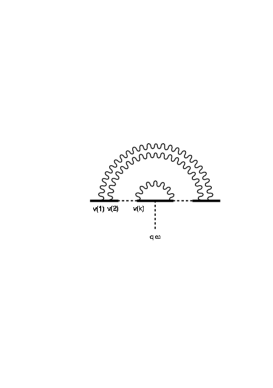
Figure 28: General form of higher order correction to the vertex part.

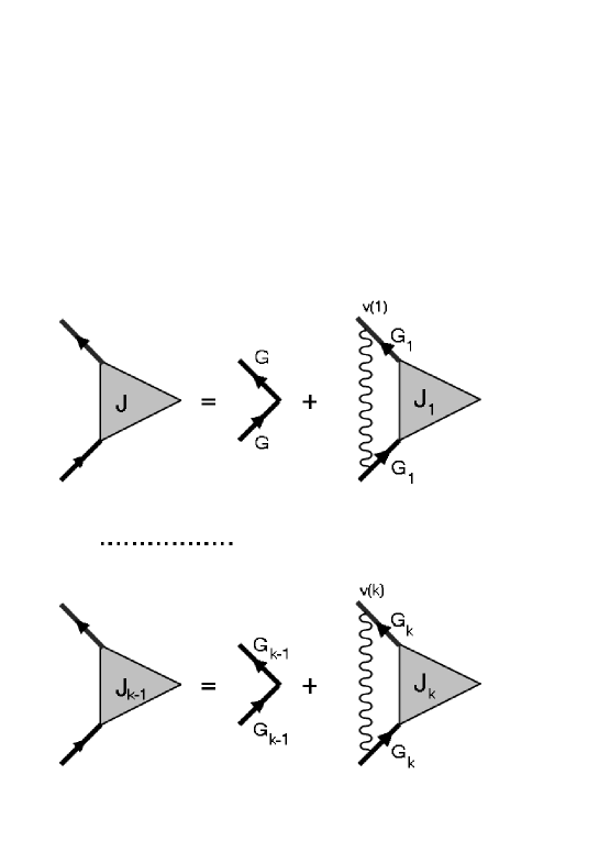
Figure 29: Recursion relations for the vertex part.

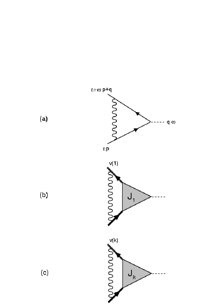
Figure 30: Simplest corrections to the vertex parts.

Now we immediately obtain the system of recursion equations for the vertex parts, shown graphically in Fig. 29. To obtain appropriate analytic expressions, consider the simplest vertex correction, shown in Fig. 30 (a). Performing calculations for $T=0$ in $RA$ – channel, we can easily obtain its contribution as:

$${\cal J}_{1}^{(1)RA}(\varepsilon{\bf p};\varepsilon+\omega{\bf p+q})=\sum_{\bf K}V_{eff}({\bf K})G_{00}^{A}(\varepsilon\xi_{\bf p-K})G_{00}^{R}(\varepsilon+\omega\xi_{\bf p-K+q})=$$

$$=W^{2}\left\{G_{00}^{A}(\varepsilon,\xi_{1}({\bf p})+iv_{1}\kappa)-G_{00}^{R}(\varepsilon+\omega,\xi_{1}({\bf p+q})-iv_{1}\kappa)\right\}\frac{1}{\omega+\xi_{1}({\bf p})-\xi_{1}({\bf p+q})}=$$

$$=W^{2}G_{00}^{A}(\varepsilon,\xi_{1}({\bf p})+iv_{1}\kappa)G_{00}^{R}(\varepsilon+\omega,\xi_{1}({\bf p+q})-iv_{1}\kappa)\left\{1+\frac{2iv_{1}\kappa}{\omega+\xi_{1}({\bf p})-\xi_{1}({\bf p+q})}\right\}\equiv$$

$$\equiv W^{2}G_{01}^{A}(\varepsilon,\xi_{\bf p})G_{01}^{R}(\varepsilon+\omega,\xi_{\bf p+q})\left\{1+\frac{2iv_{1}\kappa}{\omega+\xi_{1}({\bf p})-\xi_{1}({\bf p+q})}\right\}$$ (52)

where, during calculations of integrals, we have used the following identity, valid for free – particle Green’s functions:

$$G_{00}^{A}(\varepsilon\xi_{\bf p})G_{00}^{R}(\varepsilon+\omega\xi_{\bf p+q})=\left\{G_{00}^{A}(\varepsilon\xi_{\bf p})-G_{00}^{R}(\varepsilon+\omega\xi_{\bf p+q})\right\}\frac{1}{\omega-\xi_{\bf p+q}+\xi_{\bf p}}$$ (53)

“Dressing” internal electronic lines we obtain diagram, shown in Fig. 30 (b), and using the identity:

$$G^{A}(\varepsilon\xi_{\bf p})G^{R}(\varepsilon+\omega\xi_{\bf p+q})=\left\{G^{A}(\varepsilon\xi_{\bf p})-G^{R}(\varepsilon+\omega\xi_{\bf p+q})\right\}\times$$

$$\times\frac{1}{\omega-\xi_{\bf p+q}+\xi_{\bf p}-\Sigma^{R}_{1}(\varepsilon+\omega\xi_{\bf p+q})+\Sigma^{A}_{1}(\varepsilon\xi_{\bf p})}$$ (54)

valid for full Green’s functions, we can write down the contribution of this diagram as:

$${\cal J}_{1}^{RA}(\varepsilon{\bf p};\varepsilon+\omega{\bf p+q})=W^{2}v(1)G_{1}^{A}(\varepsilon,\xi_{\bf p})G_{1}^{R}(\varepsilon+\omega,\xi_{\bf p+q})\Biggl{\{}1+$$

$$\left.+\frac{2iv_{1}\kappa}{\omega-\xi_{1}({\bf p+q})+\xi_{1}({\bf p})-\Sigma_{2}^{R}(\varepsilon+\omega\xi_{\bf p+q})+\Sigma^{A}_{2}(\varepsilon\xi_{\bf p})}\right\}J_{1}^{RA}(\varepsilon{\bf p};\varepsilon+\omega{\bf p+q})$$

(55)

Here we assumed, that interaction line in the vertex correction diagram of Fig. 30 (b) “transforms” self – energies $\Sigma_{1}^{R,A}$ of internal electronic lines into $\Sigma_{2}^{R,A}$, in accordance with our main approximation for self – energies used above (cf. Fig. 23).

Now it is not difficult to write down similar expression for the diagram of general form, shown in Fig. 30 (c):

$${\cal J}_{k}^{RA}(\varepsilon{\bf p};\varepsilon+\omega{\bf p+q})=W^{2}v(k)G_{k}^{A}(\varepsilon,\xi_{\bf p})G_{k}^{R}(\varepsilon+\omega,\xi_{\bf p+q})\Biggl{\{}1+$$

$$\left.+\frac{2iv_{k}\kappa k}{\omega-\xi_{k}({\bf p+q})+\xi_{k}({\bf p})-\Sigma_{k+1}^{R}(\varepsilon+\omega\xi_{\bf p+q})+\Sigma^{A}_{k+1}(\varepsilon\xi_{\bf p})}\right\}J_{k}^{RA}(\varepsilon{\bf p};\varepsilon+\omega{\bf p+q})$$

(56)

Accordingly, we can write dowm the following fundamental recursion relation for the vertex part, shown in Fig. 23:

$$J_{k-1}^{RA}(\varepsilon{\bf p};\varepsilon+\omega{\bf p+q})=1+W^{2}v(k)G_{k}^{A}(\varepsilon,\xi_{\bf p})G_{k}^{R}(\varepsilon+\omega,\xi_{\bf p+q})\Biggl{\{}1+$$

$$\left.+\frac{2iv_{k}\kappa k}{\omega-\xi_{k}({\bf p+q})+\xi_{k}({\bf p})-\Sigma_{k+1}^{R}(\varepsilon+\omega\xi_{\bf p+q})+\Sigma^{A}_{k+1}(\varepsilon\xi_{\bf p})}\right\}J_{k}^{RA}(\varepsilon{\bf p};\varepsilon+\omega{\bf p+q})$$

(57)

“Physical” vertex $J^{RA}(\varepsilon{\bf p};\varepsilon+\omega{\bf p+q})$ is defined as $J^{RA}_{k=0}(\varepsilon{\bf p};\varepsilon+\omega{\bf p+q})$. Recursion procedure (57) takes into account all diagrams of perturbation theory for the vertex part. For $\kappa\to 0\quad(\xi\to\infty)$ (57) redoces to the series. studied in Refs. [51] (see also Ref. [47]), which can be summed exactly in analytic form. Standard “ladder” approximation is obtained from our scheme putting all combinatorial factors $v(k)$ in (57) to unity [65].

Conductivity is expressed via retarded density – density response function $\chi^{R}(q\omega)$ [67]:

$$\sigma(\omega)=e^{2}\lim_{q\to 0}\left(-\frac{i\omega}{q^{2}}\right)\chi^{R}(q\omega)$$ (58)

where $e$ is electronic charge,

$$\chi^{R}(q\omega)=\omega\left\{\Phi^{RA}(0q\omega)-\Phi^{RA}(00\omega)\right\}$$ (59)

where two – particle Green’s function $\Phi^{RA}(\varepsilon q\omega)$ is defined by loop diagram shown in Fig. 31.

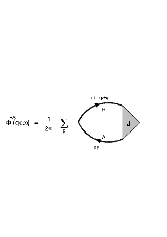
Figure 31: Diagrammatic representation for two – particle function $\Phi^{RA}(q\omega)$.

Direct numerical computations confirm, that the recurrence procedure (57) satisfies an exact relation, which directly follows (for $\omega\to 0$) from the Ward identity [67]:

$$\Phi^{RA}(00\omega)=-\frac{N(E_{F})}{\omega}$$ (60)

where $N(E_{F})$ is the density of states at the Fermi level $E_{F}=\mu$. Actually, this is our main motivation for the Ansatz, used during the derivation of (55), (56) and (57).

Finally, conductivity is written in the following symmetrized form, convenient for numerical computations:

$$\sigma(\omega)=\frac{e^{2}\omega^{2}}{\pi}\lim_{q\to 0}\frac{1}{q^{2}}\sum_{\bf p}\left\{G^{R}\left(\frac{\omega}{2},{\bf p}+\frac{{\bf q}}{2}\right)J^{RA}\left(\frac{\omega}{2},{\bf p}+\frac{{\bf q}}{2};-\frac{\omega}{2},{\bf p}-\frac{{\bf q}}{2}\right)G^{A}\left(-\frac{\omega}{2},{\bf p}-\frac{{\bf q}}{2}\right)-\right.$$

$$\left.-G^{R}\left(\frac{\omega}{2},{\bf p}\right)J^{RA}\left(\frac{\omega}{2},{\bf p};-\frac{\omega}{2},{\bf p}\right)G^{A}\left(-\frac{\omega}{2},{\bf p}\right)\right\}$$

(61)

where we also accounted for an extra factor of 2, due to summation over spin.

Direct numerical calculations [66] were performed, for different values of parameters of the “bare” spectrum (10), using (61), (57), (44), with recursion procedure starting at some high value of $k$, where all $\Sigma_{k}$ and $J_{k}$ were assumed to be zero. Integration in (61) was made over the Brillouin zone. Integration momenta are naturally made dimensionless with the help of lattice constant $a$, all energies below are given in units of transfer integral $t$. Conductivity is measured in units of universal conductivity of two – dimensional system: $\sigma_{0}=\frac{e^{2}}{\hbar}=2.5\ 10^{-4}$ Ohm^-1, and density of states — in units of $1/ta^{2}$. For definiteness, below we always take $W=t$.

First let us consider Fermi surfaces close to the case of half – filled band $\mu=0$ and $t^{\prime}=0$, shown (in the first quadrant of Brillouin zone) in Fig. 32 (a).

Figure 32: Fermi surfaces for different values of $t^{\prime}$ and chemical potential $\mu$. (a) corresponds to $\mu=0$ and the following values of $t^{\prime}/t$: 0 – I; -0.2 – II; -0.4 – III; -0.6 – IV. (b) corresponds to $t^{\prime}=0$ and the following values of $\mu/t$: 0 – I; -0.3 – II; -0.5 – III; -0.6 – IV. At the inserts we show energy dependences of spectral densities for spin – fermion model for $\kappa a=0.1$ at points of the momentum space denotes by stars.

We know that for $\mu=0$ and $t^{\prime}=0$ Fermi surface is simply square (complete ”nesting”), so that we practically are dealing with one – dimensional case, analyzed long ago in Refs. [51, 64, 65]. Results of our calculations for real part of optical conductivity in our two – dimensional model, for the case of spin – fermion diagram combinatorics and different values of correlation length of AFM short – range order (parameter $\kappa=\xi^{-1}$, where $\xi$ is measured in units of lattice constant $a$) are shown in Fig. 33.

Figure 33: Real part of optical conductivity in spin – fermion model for the case of square Fermi surface ($\mu=0$, $t^{\prime}=0$) for different values of inverse correlation length ${\kappa a}$: 0.1 – 1; 0.2 – 2; 0.5 – 3. At the insert we show appropriate densities of states.

Qualitative behavior of conductivity is quite similar to those found for one – dimensional model (for the case of incommensurate fluctuations of CDW – type) in Refs. [64, 65]. It is characterized by the presence of large pseudogap absorption maximum (appropriate densities of states with pseudogap close to the Fermi level are shown at the insert in Fig. 33) at $\omega\sim 2W$ and also by a maximum at small frequencies, connected with carrier localization in static (in our approximation) random field of AFM fluctuations. Localization nature of this maximum is confirmed by its transformation into characteristic “Drude – like” peak (with maximum at $\omega=0$) if we perform calculations in “ladder” approximation, when combinatorial factors $v(k)=1$, which corresponds to “switching off” the contribution from diagrams with intersecting interaction lines, leading to two – dimensional Anderson localization [67, 68]. Qualitative form of conductivity in this case is also quite similar to those found in Ref. [65]. Narrowing of localization peak with diminishing correlation length of fluctuations can be explained, as was noted in Ref. [65], by suppression of effective interaction (15) for small $\xi$ (with fixed value of $W$), leading to general suppression of scattering, also on the “cold” part of the Fermi surface. Note that general behavior of the density of states and optical conductivity obtained here is in complete qualitative agreement with the results, obtained for the similar two – dimensional model of Peierls transition by quantum Monte – Carlo calculations in Ref. [69].

Now, if we keep $\mu=0$ and “switch on” the transfer integral $t^{\prime}$ between second nearest neighbors in (10), we shall obtain Fermi surfaces different from square one, as shown in Fig. 32 (a). At the insert on this figure we also show the energy dependence of spectral density (50) at several typical points on these Fermi surfaces. It is seen that spectral density demonstrates characteristic “non Fermi – liquid” behavior, of the type studied in Refs. [47, 48], practically everywhere on the Fermi surface, until this surface is not very different from the square, despite the fact that the “hot spot” in this case lies precisely at the intersection of the Fermi surface with diagonal of the Brillouin zone. Appropriate dependences of the real part of optical conductivity are shown in Fig. 34.

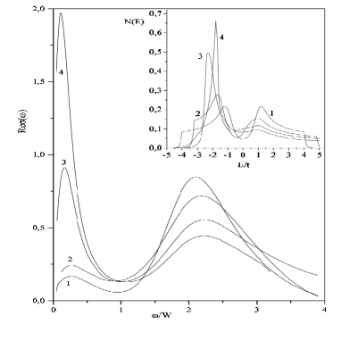
Figure 34: Real part of optical conductivity in spin – fermion model for $\mu=0$ and ${\kappa a}=0.1$ and for different Fermi surfaces, obtained from the square after “switching on” the transfer integral $t^{\prime}/t$: 0 – 1; -0.2 – 2; -0.4 – 3; -0.6 – 4. At the insert — appropriate densities of states.

At the insert in this figure we show appropriate densities of states. It is seen that as we move away from the complete “nesting”, pseudogap absorption maximum becomes more shallow, while localization peak (in accordance with the general sum rule for conductivity) grows. Note, however, that pseudogap absorption remains noticeable even when pseudogap in the density of states is practically invisible (curves 4 in Fig. 34).

Let us return now to the case of $t^{\prime}=0$ and change the value of $\mu$, so that Fermi surfaces are close to the square, as shown in Fig. 32 (b). Strictly speaking, “hot spots” on these surfaces are absent, but spectral density shown at the insert on Fig. 32 (b), is still typically pseudogap like. Appropriate dependences of the real part of optical conductivity are shown in Fig. 35.

Figure 35: Real part of optical conductivity in spin – fermion model for $t^{\prime}=0$ and ${\kappa a}=0.1$ and for different Fermi surfaces, obtained from square as we move from the case of half – filled band. Chemical potential $\mu/t$: 0 – 1; -0.3 – 2; -0.5 – 3; -0.6 – 4.

Consider now geometry of the Fermi surface with “hor spots” typical for most of HTSC – oxides, like that shown in Fig. 14. First, in Fig. 36 we show the real part of optical conductivity, calculated (for different combinatorics of diagrams) for characteristic value of $t^{\prime}=-0.4t$ and for chemical potential $\mu=0$, when “hot spots” are on the diagonals of the Brillouin zone. It is seen that pseudogap behavior of conductivity is conserved even in the case of practically absent pseudogap in the density of states (shown at the insert in Fig. 36).

Figure 36: Real part of optical conductivity for $t^{\prime}/t=-0.4$ and $\mu=0$ for ${\kappa a}=0.1$ and for different combinatorics of diagrams: 1 – spin – fermion combinatorics; 2 – commensurate case. Dashed curve — “ladder” approximation. At the insert — appropriate densities of states.

Dashed curve in Fig. 36 shows the result of “ladder” approximation, demonstrating disappearance of two – dimensional localization. In general, as correlation length of the short – range order diminishes, we observe “smearing” of the pseudogap maximum in conductivity.

For most copper oxide superconductors characteristic geometry of the Fermi surface can be described by $t^{\prime}=-0.4t$ and $\mu=-1.3t$ [47]. In this case, results of our calculations of optical conductivity for different values of inverse correlation length $\kappa$ are shown in Fig. 37 (for the case of spin – fermion combinatorics).

Figure 37: Real part of optical conductivity in spin – fermion model for $t^{\prime}/t=-0,4$ and $\mu/t=-1.3$ and for different values of correlation length ${\kappa a}$: 0.05 – 1; 0.1 – 2; 0.2 – 3. Damping factor ${\gamma/t}=0.005$.

here we introduced additional weak scattering due to inelastic processes via standard replacement $\omega\to\omega+i\gamma$ [70], which leads to the appearance of a narrow “Drude – like” peak for $\omega<\gamma$ (destruction of two – dimensional localization due to phase decoherence). It is easy to see that with the growth of inelastic scattering rate $\gamma$, localization peak is completely “smeared” and transformed to the “usual” Drude – like peak at small frequencies. Pseudogap absorption maximum becomes more pronounced with the growth of correlation length $\xi$ (diminishing $\kappa$). Similar results for the “hot patches” model were obtained in Ref. [71]

Direct correspondence of these results with experimental data shown in Fig. 4 [28] is obvious. Simple estimates show that characteristic values of conductivity in theory and experiment are also of the same order of magnitude. In principle, it is quite possible to make quantitative fit to the experiment, varying parameters of our model.

5.3 Interaction vertex for superconducting fluctuations.

Now we are going to discuss superconductivity formation on the “background” of pseudogap fluctuations. To take into account pseudogap fluctuations during the analysis of Cooper instability and derivation of Ginzburg – Landau expansion we need knowledge of the vertex part, describing electron interaction with an arbitrary fluctuation of superconducting order parameter (gap) of a given symmetry [72]:

$$\Delta({\bf p},{\bf q})=\Delta_{\bf q}e({\bf p})$$ (62)

where the symmetry factor determining the type (symmetry) of pairing is:

$$e({\bf p})=\left\{\begin{array}[]{ll}1&(\mbox{ $s$ -- wave pairing})\\ \cos p_{x}a-\cos p_{y}a&(\mbox{ $d_{x^{2}-y^{2}}$ -- pairing})\end{array}.\right.$$ (63)

and we always assume singlet pairing.

Almost immediately we can write down recursion relations [72, 73] for “triangular” vertices in Cooper channel, similar to those introduced above during the analysis of response to electromagnetic field [66]. The vertex part of interest to us can be defined as:

$$\Gamma(\varepsilon_{n},-\varepsilon_{n},{\bf p},{\bf-p+q})\equiv\Gamma_{\bf p}(\varepsilon_{n},-\varepsilon_{n},{\bf q})e({\bf p})$$ (64)

Then $\Gamma_{\bf p}(\varepsilon_{n},-\varepsilon_{n},{\bf q})$ is determined by the recursion procedure of the following form:

$$\Gamma_{{\bf p}k-1}(\varepsilon_{n},-\varepsilon_{n},{\bf q})=1\pm W^{2}r(k)G_{k}(\varepsilon_{n},{\bf p+q})G_{k}(-\varepsilon_{n},{\bf p})\Biggl{\{}1+$$

$$+\frac{2ik\kappa v_{k}}{G^{-1}_{k}(\varepsilon_{n},{\bf p+q})-G^{-1}_{k}(-\varepsilon_{n},{\bf p})-2ik\kappa v_{k}}\Biggr{\}}\Gamma_{{\bf p}k}(\varepsilon_{n},-\varepsilon_{n},{\bf q})$$ (65)

which is represented by diagrams shown in Fig. 38.

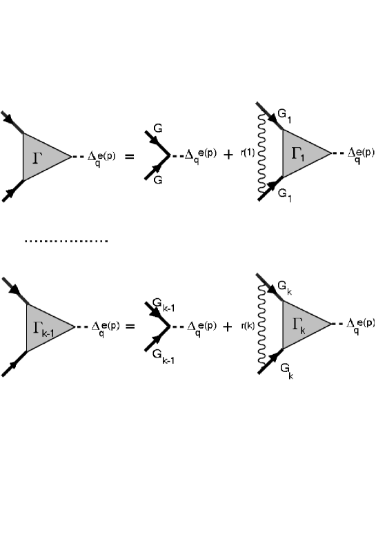
Figure 38: Recursion equations for “triangular” vertex in Cooper channel.

“Physical” vertex corresponds to $\Gamma_{{\bf p}k=0}(\varepsilon_{n},-\varepsilon_{n},{\bf q})$. Additional combinatorial factor $r(k)=v(k)$ for the simplest case of charge (or Ising like spin) pseudogap fluctuations analyzed in Ref. [72]. For the most interesting case of Heisenberg spin (SDW) fluctuations, which are mainly considered below, this factor is given by [47, 73]:

$$r(k)=\left\{\begin{array}[]{ll}k&\mbox{for even $k$}\\ \frac{k+2}{9}&\mbox{for odd $k$}\end{array}\right.$$ (66)

The choice of the sign before $W^{2}$ in the r. h. s. of (65) depends on the symmetry of superconducting order parameter and the type of pseudogap fluctuations [72, 73]. Summary of all variants is given in Table I.

Table I. The choice of sign in recursion procedure for the vertex part. Pairing CDW SDW (Ising) SDW (Heisenberg) $s$ $+$ $-$ $+$ $d$ $-$ $+$ $-$

From this table we can see, that in most interesting case of $d$ – wave pairing and Heisenberg pseudogap fluctuations this sign is “$-$”, so that we have recursion procedure with alternating signs. At the same time, for the case of $s$ – wave pairing and the same type of fluctuations we have to take this sign “$+$” and signs in recursion procedure are always the same. In Ref. [72] it was shown that this difference in types of recursion procedure leads to two different variants of qualitatively different behavior of all the main characteristics of superconductors.

5.4 Impurity scattering.

Scattering by normal (nonmagnetic) impurities is easily taken into account in self – consistent Born approximation, writing down “Dyson’s equation” shown diagrammatically in Fig. 39 (a), where in addition to Fig. 38, we have added impurity scattering contribution to electron self – energy.

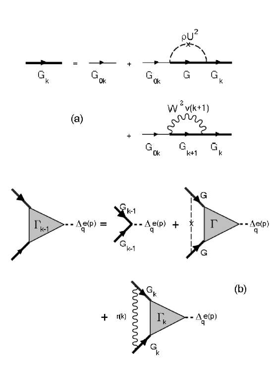
Figure 39: Recursion equations for the Green’s function (a) and “triangular” vertex (b) with the account of scattering by impurities.

As a result, recursion equation for the Green’s function is written as:

$$G_{k}(\varepsilon_{n}{\bf p})=\frac{1}{G^{-1}_{0k}(\varepsilon_{n}{\bf p})-\rho U^{2}\sum_{\bf p}G(\varepsilon_{n}{\bf p})-W^{2}v(k+1)G_{k+1}(\varepsilon_{n}{\bf p})}$$ (67)

where $\rho$ is the concentration of impurities with point – like potential $U$, and impurity scattering self – energy contains full Green’s function $G(\varepsilon_{n}{\bf p})=G_{k=0}(\varepsilon_{n}{\bf p})$, which is to be determined self – consistently by our recursion procedure. A contribution to impurity scattering self – energy form the real part of Green’s function reduces, as usual, to irrelevant renormalization of the chemical potential, so that (67) reduces to:

$$G_{k}(\varepsilon_{n}{\bf p})=\frac{1}{i(\varepsilon_{n}-\rho U^{2}\sum_{\bf p}ImG(\varepsilon_{n}{\bf p})+kv_{k}\kappa)-\xi_{k}({\bf p})-W^{2}v(k+1)G_{k+1}(\varepsilon_{n}{\bf p})}$$ (68)

Thus, in comparison with impurity free case, we have just a substitution (renormalization):

$$\varepsilon_{n}\to\varepsilon_{n}-\rho U^{2}\sum_{\bf p}ImG(\varepsilon_{n}{\bf p})\equiv\varepsilon_{n}\eta_{\epsilon}$$ (69)

$$\eta_{\epsilon}=1-\frac{\rho U^{2}}{\varepsilon_{n}}\sum_{\bf p}ImG(\varepsilon_{n}{\bf p})$$ (70)

If we do not perform fully self – consistent calculations of impurity self – energy, in the simplest approximation we simply have:

$$\varepsilon_{n}\to\varepsilon_{n}-\rho U^{2}\sum_{\bf p}ImG_{00}(\varepsilon_{n}{\bf p})\equiv\varepsilon_{n}\eta_{\epsilon}=\varepsilon_{n}+\gamma_{0}sign\varepsilon_{n}$$ (71)

$$\eta_{\epsilon}=1+\frac{\gamma_{0}}{|\varepsilon_{n}|}$$ (72)

where $\gamma_{0}=\pi\rho U^{2}N_{0}(0)$ is the standard Born impurity scattering rate ($N_{0}(0)$ is the density of states of free electrons at the Fermi level).

For “triangular” vertices of interest to us, recursion equations with the account of impurity scattering is shown diagrammatically in Fig. 39 (b). For the vertex, describing electron interacting with superconducting order parameter fluctuation (62) with $d$ – wave symmetry (63), this equation is considerably simplified, as the contribution of the second diagram in the r. h. s. of Fig. 39 (b) in fact vanishes due to $\sum_{\bf p}e({\bf p})=0$ (cf. discussion of similar situation in Ref. [50]). Then the recursion equation for the vertex takes the form (65), where $G_{k}(\pm\varepsilon_{n}{\bf p})$ are given by (67), (68), i.e. are just Green’s functions “dressed” by impurity scattering, determined gy diagrams of Fig. 39 (a). For the vertex describing interaction with order parameter fluctuations with $s$ – wave symmetry, we have the following equation:

$$\Gamma_{{\bf p}k-1}(\varepsilon_{n},-\varepsilon_{n},{\bf q})=1+\rho U^{2}\sum_{\bf p}G(\varepsilon_{n},{\bf p+q})G(-\varepsilon_{n},{\bf p})\Gamma_{\bf p}(\varepsilon,-\varepsilon_{n},{\bf q})\pm$$

$$\pm W^{2}r(k)G_{k}(\varepsilon_{n},{\bf p+q})G_{k}(-\varepsilon_{n},{\bf p})\Biggl{\{}1+$$ (73)

$$+\frac{2ik\kappa v_{k}}{G^{-1}_{k}(\varepsilon_{n},{\bf p+q})-G^{-1}_{k}(-\varepsilon_{n},{\bf p})-2ik\kappa v_{k}}\Biggr{\}}\Gamma_{{\bf p}k}(\varepsilon_{n},-\varepsilon_{n},{\bf q})$$

where $G_{k}(\pm\varepsilon_{n}{\bf p})$ is again given by (67), (68), and the sign before $W^{2}$ is determined according to the rules formulated above. The difference with the case of the vertex, describing interaction with $d$ – wave fluctuations, is in the appearance of the second term in the r. h. s. of (73), so that we have to substitute:

$$1\to\eta_{\Gamma}=1+\rho U^{2}\sum_{\bf p}G(\varepsilon_{n},{\bf p+q})G(-\varepsilon_{n},{\bf p})\Gamma_{\bf p}(\varepsilon,-\varepsilon_{n},{\bf q})$$ (74)

Now the self – consistent procedure look as follows. We start from “zeroth” approximation $G=G_{00}$, $\Gamma_{\bf p}=1$, then in Eqs. (68), (73) we just have $\eta_{\varepsilon}=\eta_{\Gamma}=1-\rho U^{2}/\varepsilon_{n}\sum_{\bf p}ImG_{00}(\varepsilon_{n}{\bf p})$. Then perform recursions (starting from some big enough value of $k$) and determine new values of $G=G_{k=0}$ and $\Gamma_{\bf p}=\Gamma_{k=0}$. Again calculate $\eta_{\varepsilon}$ and $\eta_{\Gamma}$ using (70) and (74), put these into (68), (73) etc., until convergence.

While analyzing vertices with $d$ – wave symmetry, we have simply to put $\eta_{\Gamma}=1$ at all stages of calculation. In fact, in these case there is no serious need to perform fully self – consistent calculation, because it leads only to insignificant corrections to the results of non self – consistent calculation, using only simplest substitution (71) [75].

As an illustration, in Fig. 40 we show comparison of ARPES data of Ref. [36] for momentum dependence of $a=Im\Sigma(E=0,{\bf p})$, taken from Fig. 10 (c), with the results of non self – consistent calculation using (68), (71), (72). Assumed values of parameters, typical for HTSC, are shown on the figure, for the parameters of the spectrum (10) we have taken $t=0.25eV$,  $t^{\prime}=-0.4t$, while chemical potential was calculated for two limiting doping levels. It can be seen that we obtain correct order of magnitude estimate of anisotropy in momentum space, but the general form of this dependence is only qualitatively similar to that observed in the experiment, which lies in between two calculated curves. More or less similar results are obtained also in the case of spin – fermion combinatorics.

Figure 40: Comparison of ARPES data for the static contribution to the imaginary part of electron self – energy $a=Im\Sigma(E=0,{\bf p})$ with calculated results for the “hot spots” model with impurity scattering, for typical set of model parameters, shown in the figure. Shown are the results for commensurate combinatorics and two values of doping: $0\%$ and $20\%$. Momentum $k_{x}$ is given in units of $\frac{\pi}{a}$, and its change between 0 and 1 corresponds to measurement point moving along the Fermi surface from the diagonal of the Brillouin zone towards the vicinity of the point $(0,\pi)$.

In principle, rather approximate agreement of calculated results with experiment is not very surprising. Our model is certainly oversimplified, and experimental data are also not very precise. Besides, we practically know nothing about the values of parameters of the model, appropriate for the system, studied in these experiments.

5.5 Superconducting transition temperature and Ginzburg – Landau expansion.

Critical temperature of superconducting transition is determined by the equation for Cooper instability of the normal phase:

$$1-V\chi(0;T)=0$$ (75)

where generalized Cooper susceptibility is defined by diagram shown in Fig. 41 and is equal to:

$$\chi({\bf q};T)=-T\sum_{\varepsilon_{n}}\sum_{\bf p}G(\varepsilon_{n}{\bf p+q})G(-\varepsilon_{n},-{\bf p})e^{2}({\bf p})\Gamma_{\bf p}(\varepsilon_{n},-\varepsilon_{n},{\bf q})$$ (76)

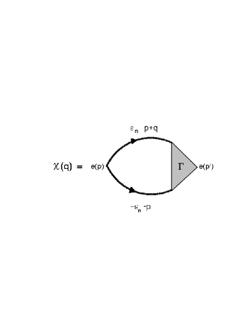
Figure 41: Diagrammatic representation for generalized susceptibility $\chi({\bf q})$ in Cooper channel.

Pairing coupling constant $V$ is assumed to be nonzero in some layer of the width of $2\omega_{c}$ around the Fermi level and determines the “bare” transition temperature $T_{c0}$ in the absence of the pseudogap fluctuations via standard BCS equation:

$$1=\frac{2VT}{\pi^{2}}\sum_{n=0}^{\bar{m}}\int_{0}^{\pi/a}dp_{x}\int_{0}^{\pi/a}dp_{y}\frac{e^{2}({\bf p})}{\xi^{2}_{\bf p}+\varepsilon^{2}_{n}}$$ (77)

where $\bar{m}=[\frac{\omega_{c}}{2\pi T_{c0}}]$ is dimensionless cut – off parameter of the sum over Matsubara frequencies. All calculations [72, 73] were performed for the typical spectrum of quasiparticles (10), for different relations between $t$, $t^{\prime}$ and $\mu$. Choosing, rather arbitrarily, $\omega_{c}=0.4t$ and $T_{c0}=0.01t$, we can easily find the appropriate value of pairing interaction $V$ in (77), leading to this given value of $T_{c0}$ for different types of pairing. In particular, for $t^{\prime}/t=-0.4$, $\mu/t=-1.3$ and for $s$ – wave pairing we get $\frac{V}{ta^{2}}=1$, while for $d_{x^{2}-y^{2}}$ – pairing we obtain $\frac{V}{ta^{2}}=0.55$.

To determine $T_{c}$ we need only the knowledge of Cooper susceptibility for $q=0$ which considerably simplifies all calculations [72]. In general case, e.g. to derive coefficients of Ginzburg – Landau expansion we need to know $\chi(q;T)$ for arbitrary (small) $q$.

Ginzburg – Landau expansion for the difference of free energies of superconducting and normal states is written in the following standard form:

$$F_{s}-F_{n}=A|\Delta_{\bf q}|^{2}+q^{2}C|\Delta_{\bf q}|^{2}+\frac{B}{2}|\Delta_{\bf q}|^{4}$$ (78)

and is determined by the loop expansion of free energy of an electron in the field of fluctuations of suoerconducting order parameter (62), shown in Fig. 42.

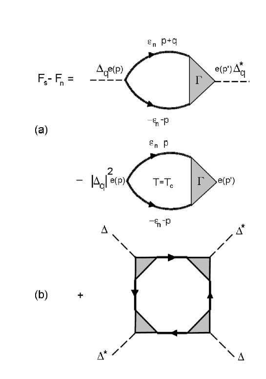
Figure 42: Diagrammatic representation of Ginzburg – Landau expansion.

It is convenient to normalize Ginzburg – Landau coefficients $A,B,C$ by their values in the absence of pseudogap fluctuations, writing the following representation [72]:

$$A=A_{0}K_{A};\qquad C=C_{0}K_{C};\qquad B=B_{0}K_{B},$$ (79)

$$A_{0}=N_{0}(0)\frac{T-T_{c}}{T_{c}}<e^{2}({\bf p})>;\quad C_{0}=N_{0}(0)\frac{7\zeta(3)}{32\pi^{2}T_{c}^{2}}<|{\bf v}({\bf p})|^{2}e^{2}({\bf p)}>;$$

$$B_{0}=N_{0}(0)\frac{7\zeta(3)}{8\pi^{2}T_{c}^{2}}<e^{4}({\bf p})>,$$ (80)

where the angular brackets denote the usual averaging over the Fermi surface: $<\ldots>=\frac{1}{N_{0}(0)}\sum_{p}\delta(\xi_{\bf p})\ldots$, where $N_{0}(0)$ – density of states on the Fermi level for free electrons.

Then we obtain the following general expressions [72]:

$$K_{A}=\frac{\chi(0;T)-\chi(0;T_{c})}{A_{0}}$$ (81)

$$K_{C}=\lim_{q\to 0}\frac{\chi({\bf q};T_{c})-\chi(0;T_{c})}{q^{2}C_{0}}$$ (82)

$$K_{B}=\frac{T_{c}}{B_{0}}\sum_{\varepsilon_{n}}\sum_{\bf p}e^{4}({\bf p})(G(\varepsilon_{n}{\bf p})G(-\varepsilon_{n},-{\bf p}))^{2}(\Gamma_{\bf p}(\varepsilon_{n},-\varepsilon_{n},0))^{4}$$ (83)

which were used for direct numerical calculations. In the presence of impurities all Green’s functions and vertices, entering these expressions, should be calculated using Eqs. (68) and (73), derived above.

The knowledge of the coefficients of Ginzburg – Landau expansion allows to determination of all major characteristics of a superconductor close to the transition temperature $T_{c}$. Coherence length is defined as:

$$\frac{\xi^{2}(T)}{\xi_{BCS}^{2}(T)}=\frac{K_{C}}{K_{A}},$$ (84)

where $\xi_{BCS}(T)$ is the value of this length in the absence of the pseudogap. Penetration depth is:

$$\frac{\lambda(T)}{\lambda_{BCS}(T)}=\left(\frac{K_{B}}{K_{A}K_{C}}\right)^{1/2},$$ (85)

where we again normalized to the value of $\lambda_{BCS}(T)$ in the absence of pseudogap fluctuations. Analogously, normalized slope of the upper critical field close to $T_{c}$ is:

$$\frac{\left|\frac{dH_{c2}}{dT}\right|_{T_{c}}}{\left|\frac{dH_{c2}}{dT}\right|_{T_{c0}}}=\frac{T_{c}}{T_{c0}}\frac{K_{A}}{K_{C}}.$$ (86)

Specific heat discontinuity at the transition:

$$\Delta C=\frac{(C_{s}-C_{n})_{T_{c}}}{(C_{s}-C_{n})_{T_{c0}}}=\frac{T_{c}}{T_{c0}}\frac{K_{A}^{2}}{K_{B}}.$$ (87)

Results of these calculations for the cases of charge (CDW) and Ising like spin (SDW) fluctuations of short range order can be found in Ref. [72]. Here we shall concentrate mainly on the analysis of most important and interesting case of Heisenberg spin (SDW) fluctuations and also on the discussion of the role of impurity scattering (disordering) [73, 74]. Due to particular importance of the case of $d$ – wave pairing in the physics of copper oxide high – temperature superconductors, more attention will be given to this case.

In the following we give the results of calculations made for typical values of spectrum parameters $t^{\prime}/t=-0.4$, $\mu/t=-1.3$, while for correlation length we assume $\kappa a=0.2$. To spare space we do not show the results for dimensionless GL – coefficients $K_{A},\ K_{B},\ K_{C}$, but restrict ourselves to demonstration of more important dependences of all major physical characteristics.

When we are dealing with dependences on the effective width of the pseudogap, all characteristics are normalized to their values at $T=T_{c0}$, while in case of dependences on the impurity scattering rate $\gamma_{0}$ we normalize to the values at $T=T_{c0}(W)$, i.e. at the value of the “bare” transition temperature at a given value of $W$, but in the absence of impurity scattering ($\gamma_{0}=0$).

5.5.1 $d$ – wave pairing.

In Fig. 43 we show the dependence of superconducting transition temperature $T_{c}$ on the effective pseudogap width $W$ for several values of impurity scattering rate. It is seen that pseudogap fluctuations lead to significant suppression of superconductivity, and in the presence of finite disorder we always obtain some “critical” value of $W$, where the value of $T_{c}$ vanishes. This suppression of $T_{c}$ is naturally due to a partial “dielectrization” of electronic spectrum in the vicinity of “hot spots”. [47, 48].

Figure 43: Dependence of $T_{c}$ on the effective width of the pseudogap $W$ in the case of $d$ – wave pairing, for several values of impurity scattering rate $\gamma_{0}/T_{c0}$: 0 – 1; 0.18 – 2; 0.64 – 3. Inverse correlation length $\kappa a$=0.2

Similar dependences for the slope of the upper critical field and specific heat discontinuity at the transition point are shown in Fig. 44. Typically we see fast suppression of these characteristics by pseudogap fluctuations.

Figure 44: Dependence of the slope of the upper critical field and specific heat discontinuity at the transition on the effective width of the pseudogap $W$ in case of $d$ – wave pairing, for several values of impurity scattering rate $\gamma_{0}/T_{c0}$: 0 – 1; 0.18 – 2; 0.64 – 3.

Dependence on the value of correlation length of pseudogap fluctuations is more slow — in all cases the growth of $\xi$ (drop of $\kappa$) enhances the effect of pseudogap fluctuations. We drop appropriate results to spare space.

In Fig. 45 we show the dependences of superconducting transition temperature $T_{c}$ on impurity scattering rate $\gamma_{0}$ for several values of the effective pseudogap width. We note that in the presence of pseudogap fluctuations, suppression of $T_{c}$ by disorder is significantly faster, than in their absence ($W=0$), when $T_{c}$ dependence on $\gamma_{0}$ in case of $d$ – wave pairing is described by the standard Abrikosov – Gorkov curve (first obtained for $s$ – wave pairing and scattering by magnetic impurities) [76, 77]. Similar dependences for the slope of $H_{c2}(T)$ and specific heat discontinuity are shown in Fig. 46. Again we see, that impurity scattering (disorder) leads to the fast drop of these two characteristics, i.e. enhances similar effect of pseudogap fluctuations.

Figure 45: Dependence of $T_{c}$ on impurity scattering rate (disorder) $\gamma_{0}$ for the case of $d$ – wave pairing, for several values of the effective pseudogap width: $W/T_{c0}$: 0 – 1; 2.8 – 2; 5.5 – 3.

Figure 46: Dependence of the slope of the upper critical field and specific heat discontinuity at the transition on impurity scattering rate (disorder) $\gamma_{0}$ in case of $d$ – wave pairing, for several values of effective pseudogap width $W/T_{c0}$: 0 – 1; 2.8 – 2; 5.5 – 3.

Similar dependences were obtained in Ref. [72] for the case of pseudogap fluctuations of CDW type, when we also obtain recursion procedure for the vertex part wit alternating signs. At the same time, in this case we observe some quantitative difference in the behavior of all characteristics due to another combinatorics of diagrams.

Dependences obtained in our model are in qualitative agreement with most of the experimental data on superconductivity in the pseudogap region (underdoped region of the phase diagram of cuprates). Below we shall show that these results may be used for direct modelling of a typical phase diagram of a high – temperature superconductor.

5.5.2 $s$ – wave pairing.

The case of $s$ – wave pairing is interesting to us mainly with the aim of demonstration of major differences from the case of $d$ – wave case. There are no experimental evidence for $s$ – wave superconductivity in systems with pseudogap, though such systems may well be discovered in some future.

Our calculation show that pseudogap fluctuations suppress superconducting transition temperature also in this case (Fig. 47), though characteristic scale of these fluctuations, necessary for significant suppression of superconductivity here is much larger, than in the case of $d$ – wave pairing. This result was obtained in Ref. [72], but we must note the absence (in the case of Heisenberg (SDW) pseudogap fluctuations) of characteristic “plateau” in the dependence of $T_{c}$ on $W$, which was obtained for the case of scattering by pseudogap fluctuations of CDW type in Ref. [72]. On the same scale of $W$ we also observe here the suppression of specific heat discontinuity at the transition, which is shown at the insert in Fig. 47.

Figure 47: Dependence of $T_{c}$ on effective width of the pseudogap $W$ for the case of $s$ – wave pairing, for two values of impurity scattering rate: $\gamma_{0}/T_{c0}$: 0 – 1; 20 – 2. Inverse correlation length $\kappa a$=0.2. At the insert – characteristic behavior of specific heat discontinuity for the same parameters.

As to dependence of $T_{c}$ on impurity scattering rate (disorder), we can see that besides relatively small effect of $T_{c}$ suppression due to [75] disorder “smearing” of the density of states at the Fermi level, even some weak effect of $T_{c}$ enhancement with the growth of $\gamma_{0}$ can be also observed, apparently due to the “filling” the pseudogap in the density of states induced by impurity scattering [73].

In Fig. 48 we show the influence of impurity scattering (disorder) on the slope of the upper critical field and specific heat discontinuity. Specific heat discontinuity is significantly suppressed by disorder, while the slope of $H_{c2}(T)$ behaves qualitatively different from the case of $d$ – wave pairing: the growth of disorder leads to the growth of this characteristic, as in the case of standard theory of “dirty” superconductors [16], and pseudogap fluctuations enhance the slope of $H_{c2}(T)$. In the absence of pseudogap fluctuations, similar differences between $s$ – wave and $d$ – wave superconductors in behavior of the slope of $H_{c2}(T)$ under disordering were discussed in Ref. [76].

Figure 48: Dependence of the slope of the upper critical field and specific heat discontinuity at the transition on impurity scattering rate (disorder) $\gamma_{0}$ in case of $s$ – wave pairing, for two values of pseudogap width: $W/T_{c0}$: 0 – 1; 15 – 2.

6 Modeling of the phase diagram of cuprates.

This model for the influence of pseudogap fluctuations on superconductivity allows to perform a simple modeling of typical phase diagram of HTSC cuprates [73, 74] First attempt of such modeling in quite simplified version of our model was undertaken in Ref. [56]. Basic idea is to identify our parameter $W$ with experimentally observable effective width of the pseudogap (temperature of crossover into pseudogap region on the phase diagram) $E_{g}\approx T^{*}$, determined from numerous experiments [24, 21]. This characteristic, as was already noted above, drops almost linearly with the growth of the concentration of doping impurity (concentration of carriers), starting from the values of the order of $10^{3}$K and vanishing at some critical concentration $x_{c}\approx 0.19..0.22$, slightly higher than “optimal” value $x_{o}\approx 0.15..0.17$ [24, 78]. Accordingly, we can assume similar concentration dependence of our pseudogap width $W(x)$. In this sense we can say that $W(x)$ is determined directly from the experiment. Then, the only parameter we need remains concentration dependence of the “bare” temperature of superconducting transition $T_{c0}(x)$, which would have been existing in the absence of pseudogap fluctuations. Its knowledge would allow us to determine the concentration dependence of the observable transition temperature $T_{c}(x)$, solving the equations of our model. Unfortunately, concentration dependence $T_{c0}(x)$ is, generally, unknown and is not determined by any known experiment, remaining just free fitting parameter of our theory.

Following Ref. [56] we can assume, that $T_{c0}(x)$ can also be described by linear function of $x$, going to zero at $x=0.3$, and choosing the value of $T_{c0}(x=0)$, which give us experimentally observed $T_{c}(x=x_{o})$. Then we can calculate the whole “observed” dependence $T_{c}(x)$. Results of such calculation for the case of $d$ – wave pairing and scattering by charge (CDW) pseudogap fluctuations [72], using typical $W(x)$ dependence, are shown in Fig. 49.

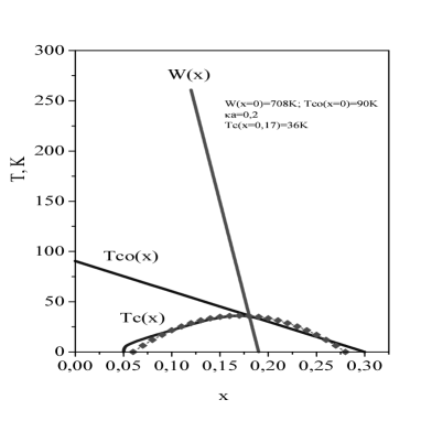
Figure 49: Model phase diagram for the case of scattering by pseudogap fluctuations of CDW – type ($d$ – wave pairing) and “bare” superconducting transition temperature $T_{c0}$ linear in carrier concentration.

We see that even with such arbitrary assumptions the “hot spots” model allows to obtain $T_{c}(x)$ dependence, which is rather close to experimentally observable. Similar calculations for Ising like model of spin fluctuations (leading to the absence of sign alternation in the recursion procedure for the vertex part [72]) show, that reasonable values for $T_{c}(x)$ can be obtained only for unrealistic values of $W(x)$, at least an order of magnitude larger than observed in the experiments.

In the framework of our BCS – like model for the “bare” $T_{c0}$, an assumption of its strong concentration dependence seems rather unrealistic. Thus, let us assume that the value of $T_{c0}$ does not depend on carrier concentration $x$ at all, but take into account the fact that introduction of doping impurity inevitably leads to appearance random impurity scattering (internal disorder), which can be described by appropriate linear dependence of $\gamma(x)$. Let us assume that it is this growth of disorder, which leads to complete suppression of $d$ – wave pairing at $x=0.3$, in accordance with Abrikosov – Gorkov dependence [76, 77]. Results of our modeling of the phase diagram for the system of the type of $La_{2-x}Sr_{x}CuO_{4}$, for the case of Heisenberg pseudogap fluctuations, with the account of the abovementioned role of internal disorder, are shown in Fig. 50.

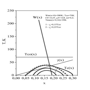
Figure 50: Model phase diagram for the case of scattering by Heisenberg (SDW) pseudogap fluctuations ($d$ – wave pairing) and “bare” temperature of superconducting transition $T_{c0}$ independent of carrier concentration, with the account of internal disorder linear in concentration of doping impurity $\gamma(x)$.

The values of different parameters used in this calculation are also shown at the same figure. “Experimental” values of $T_{c}(x)$, shown at this figure (as well as at Fig. 49) by “diamonds”, were obtained from empirical relation [78, 79]:

$$\frac{T_{c}(x)}{T_{c}(x=x_{o})}=1-82.6(x-x_{o})^{2}$$ (88)

which gives rather good fit to experimental data on concentration dependence of $T_{c}$ for a number of HTSC cuprates. It is seen, that in the whole underdoped region our model gives practically ideal description of “experimental” data with very reasonable values of $W(x)$. At the end of overdoped region agreement is less good, but you must take into account, that Eq. (88) also usually does not give very good fit here, and the obvious crudeness of our assumptions for underdoped region. Also note, that we have not undertaken any special attempts to improve agreement in this region.

It is interesting to analyze the behavior of superconducting transition temperature $T_{c}$ under additional disordering of our system at different compositions (carrier concentrations). There are many experimental studies [16], where such an additional disordering was introduced by chemical substitutions (impurities) [81, 82] or by irradiation with fast neutrons [80] or electrons [83, 84]. However, special discussion of the role of this additional disordering in the context of the studies of the pseudogap state was made only in Ref. [82].

In our model, such disordering may be simulated by introduction of additional “impurity” scattering parameter $\gamma_{0}$, which is just added to the parameter of internal disorder $\gamma(x)$. Results of our calculations of superconducting critical temperature for two values of this parameter are also shown in Fig. 50. We see, that in complete agreement with experiments [82], introduction of “impurities” (disorder) leads to fast narrowing of the superconducting region on the phase diagram. Also in complete accordance with our conclusions made above with respect to Fig. 45, and also with experiments [80, 82], superconductivity suppression by disorder in the underdoped region (pseudogap state) is significantly faster, than at optimal composition. We could have expected that introduction of “normal” disorder. obviously leading to some suppression of the pseudogap in the density of states, could also lead to certain “slowing” down of $T_{c}$ suppression. However, in case of $d$ – wave pairing, this effect is apparently absent.

The problem, however, is that in all cases our suppression of $T_{c}$ by disorder is faster than that described by the standard Abrikosov – Gorkov dependence for the case of $d$ – wave pairing [77]. At the same time, attempts to fit the results of majority of experiments on disordering in HTSC cuprates to this dependence show [81, 83, 84], that such suppression actually is significantly slower, than predicted by Abrikosov – Gorkov dependence. This, still unsolved, problem remains one of the major problems of the theory of high – temperature superconductors [16]. One possible solution may be connected with consistent description of the role of disorder in superconductors, which belong to the crossover region from “large” pairs of BCS theory to “compact” Bosons, appearing in the limit of very strong coupling [85]. Another interesting possibility to explain such “slowing down” of $T_{c}$ suppression is connected with the role of anisotropy of elastic scattering by impurities analyzed in Refs. [76, 86]. This last effect can be rather easily included in our calculational scheme. It is of particular interest in connection with established fact of rather strong anisotropy of elastic scattering (with $d$ – wave symmetry), which was observed in ARPES experiments on $Bi_{2}Sr_{2}CaCu_{2}O_{8+\delta}$ [36]. Appropriate scattering rate in these experiments changed in the interval of $20-60\ meV$ (cf. Fig. 10 (c)) [36], which is nearly an order of magnitude larger than maximal value of $\gamma(x)$, used in our calculations. This is an additional evidence of unusual stability of $d$ – wave pairing in cuprates towards static disorder. Note that our model for electron self – energy in fact describes similar anisotropy of elastic scattering, corresponding to its growth in the vicinity of “hot spots”, yet the effect of “slowing down” of $T_{c}$ suppression under disordering is not observed.

Our results show that despite the obvious crudeness of our assumptions, the “hot spots” model rather easily leads to a reasonable (sometimes even semiquantitative) description of superconductivity region on the phase diagram of HTSC cuprates. The main shortcoming this approach remains considerable arbitrariness of our “scenario” of the origin of concentration dependence of the “bare” superconducting transition temperature.

7 Conclusion.

Our discussion demonstrates the variety of results, which can be obtained in this class of models of the pseudogap state. We must stress once again quite simplified nature of our approximations, though allowing to obtain what was called “nearly exact” solution. This solution is interesting, first of all, from purely theoretical point of view, as rare enough example of the problem, when it is possible to sum the complete Feynman perturbation theory series (though, in general, certain classes of higher order diagrams are calculated approximately). Probably the main theoretical “lesson” to learn is, that the results of such complete summation are rather radically different from the results, obtained by one or other “partial” summation (e.g. of simple geometrical progression).

Probably the main shortcoming of our approach is the neglect of dynamics of fluctuations of short – range order. This is justified, as was shown above, only for high enough temperatures, which is bad, e.g. from the point of view of description of superconducting state for $T\ll T_{c}$

Another shortcoming, as was mentioned many times [57, 48], is our limitation to Gaussian fluctuations, which is also justified only for high enough temperatures. In some sense it is only technical limitation, though it is quite important for the formal structure of our solution.

We already mentioned that in this class of models we can demonstrate the breaking of the fundamental property of self – averaging of superconducting order parameter [54, 59]. Unfortunately, this can be done only in rather unrealistic case of infinite correlation length of pseudogap fluctuations [54], or in very special model with finite correlation length [58, 59], and in an oversimplified model with “hot patches” on the fermi surface. Qualitative picture emerging from this analysis demonstrates the possibility of formation of “superconducting drops” at temperatures higher than mean – field $T_{c}$ [19, 54, 59], which may have direct relation to the existence of the “low energy” pseudogap (signatures of superconducting response at $T>T_{c}$) and experimentally observed inhomogeneous superconductivity in cuprates [17, 18]. In the “hot spots” model this kind of analysis is still to be done.

At the same time, we have seen that in some cases we can make even direct comparison of predictions of these simplified models with the experiments, and the results of such comparison are rather promising. In this sense the “hot spots” model can pretend to give quasi realistic description of the properties of the pseudogap state in high – temperature superconductors.

The author is grateful to E.Z.Kuchinskii and N.A.Kuleeva (Strigina) for their collaboration during our work on the “hot spots” model. This work was supported in part by RFBR grant 02-02-16031 and programs of the Presidium of the Russian Academy of Sciences (RAS) “Quantum macrophysics” and of the Division of Physical Sciences of the RAS “Strongly correlated electrons in semiconductors, metals, superconductors and magnetic materials”.

References

- [1] J.Annett, N.Goldenfeld, A.J.Leggett. Physical Properties of High Temperature Superconductors. Vol. 5, p. 375 (Ed. by D.M.Ginsberg), World Scientific, Singapore, 1996. ArXiv: cond-mat/9601060
- [2] C.C.Tsui, J.R.Kirtley. Rev. Mod. Phys. 72, 969 (2000)
- [3] Z.-X.Shen, D.S.Dessau. Phys. Reports 253, 1 (1995)
- [4] A.Damasceli, Z.Hussain, Z.-X.Shen. Rev. Mod. Phys. 75, 475 (2003)
- [5] X.J.Zhou, T.Yoshida, D.-H.Lee, W.L.Yang, V.Brouet, F.Zhou, W.X.Ti, J.W.Xiong, Z.X.Zhao, T.Sasagawa, T.Kakeshita, H.Eisaki, S.Uchida, A.Fujimori, Z.Hussain, Z.-X.Shen. Phys. Rev. Lett. 92, 187001 (2004).
- [6] E.G.Maksimov. Physics – Uspekhi 43, 965 (2000)
- [7] M.Kuliĉ. Phys. Reports 338, 1 (2000)
- [8] M.Kuliĉ. ArXiv: cond-mat/0404287
- [9] D.J.Scalapino. Phys. Reports 250, 329 (1995)
- [10] T.Moriya, K.Ueda. Adv. Phys. 49, 555 (2000)
- [11] A.V.Chubukov, D.Pines, J.Schmalian. The Physics of Superconductors. (Ed. K.-H.Bennemann and J.B.Ketterson), Springer 2002. ArXiv: cond-mat/0201140
- [12] Y.Yanase, T.Jugo, T.Nomura, H.Ikeda, T.Hotta, K.Yamada. Phys. Reports 387, 1 (2004). ArXiv: cond-mat/0309094
- [13] P.W.Anderson. The Theory of Superconductivity in the High – Cuprates. Princeton University Press, Princeton, 1997
- [14] E.Demler, W.Hanke, Shou-Cheng Zhang. ArXiv: cond-mat/0405038
- [15] C.M.Varma, Z.Nussinov, Wim van Saarlos. Phys. Reports 361, 267 (2002)
- [16] M.V.Sadovskii. Superconductivity and Localization. World Scientific, Singapore 2000.
- [17] S.H.Pan, J.P.O’Neil, R.L.Badzey, C.Chamon, H.Ding, J.R.Engelbrecht, Z.Wang, H.Eisaki, S.Uchida, A.K.Gupta. Nature 413, 282 (2001)
- [18] K.McElroy, D.-H.Lee, J.E.Hoffman, K.M.Lang, E.W.Hudson, H.Eisaki, S.Uchida, J.Lee, J.C.Davis. ArXiv: cond-mat/0404005
- [19] L.N.Bulaevskii, S.V.Panyukov, M.V.Sadovskii. JETP 65, 380 (1987)
- [20] T.Timusk, B.Statt. Rep.Progr.Phys. 62, 61 (1999)
- [21] M.V.Sadovskii. Physics – Uspekhi 44, 5i5 (2001)
- [22] N.F.Mott, E.A.Davis. Electronic Pocesses in Non – Crystalline materials. Clarendon Press, Oxford. 1971
- [23] J.L.Tallon, J.W.Loram, Physica C349, 53 (2001), ArXiv: cond-mat/0005063
- [24] J.W.Loram, K.A.Mirza, J.R.Cooper, J.L.Tallon. Physica C 282-287, 1405 (1997)
- [25] C.Renner, B.Revaz, J.Y.Genoud, K.Kadowaki, Ø.Fisher. Phys.Rev.Lett. 80, 149 (1998)
- [26] V.M.Krasnov, A.Yurgens, D.Winkler, P.Delsing, T.Claeson. Phys.Rev.Lett. 84, 5860 (2000)
- [27] V.M.Krasnov, A.E.Kovalev, A.Yurgens, D.Winkler, Phys. Rev. Lett. 86, 2657 (2001)
- [28] Y.Onose, Y.Taguchi, K.Ishizaka, Y,Tokura. Phys. Rev. Lett. 87, 217001 (2001); Preprint (2003)
- [29] D.N.Basov, A.V.Puchkov, R.A.Hughes, T.Strach, J.Preston, T.Timusk. Phys.Rev. B49, 12165 (1994)
- [30] D.N.Basov, B.Dabrowski, T.Timusk. Phys.Rev.Lett. 81, 2132 (1998)
- [31] E.J.Singley, D.N.Basov, K.Kurahashi, T.Uefuji, K.Yamada. Phys. Rev. B64, 224503 (2001)
- [32] M.R.Norman, H.Ding, M.Randeria, J.C.Campuzano, T.Yokoya, T.Takeuchi, T.Takahashi, T.Mochiku, K.Kadowaki, P.Guptasarma, D.G.Hinks. Nature 392, 157 (1998)
- [33] H.Ding T.Yokoya, J.C.Campuzano, T.Takahashi, M.Randeria, M.R.Norman, T.Mochiku, K.Kadowaki, J.Giapintzakis. Nature 382, 51 (1996)
- [34] M.R.Norman, M.Randeria, H.Ding, J.C.Campuzano. Phys.Rev. B57, R11093 (1998)
- [35] A.Kaminski, J.Mesot, H.Fretwell, J.C.Campuzano, M.R.Norman, M.Randeria, H.Ding, T.Sato, T.Takahashi, T.Mochiku, K.Kadowaki, H.Hoechst. Phys. Rev. Lett. 84, 1788 (2000)
- [36] A.Kaminski, H.M.Fretwell, M.R.Norman, M.Randeria, S.Rosenkranz, J.C.Campuzano, J.Mesot, T.Sato, T.Takahashi, T.Terashima, M.Takano, K.Kadowaki, Z.Z.Li, H.Raffy. ArXiv: cond-mat/0404385
- [37] A.A.Kordyuk, S.V.Borisenko, A.Koitzsch, J.Fink, M.Knupfer, B.Büchner, H.Berger, G.Margaritondo, C.T.Lin, B.Keimer, S.Ono, Y.Ando. Phys. Rev. Lett. 92, 257006 (2004)
- [38] N.P.Armitage, D.H.Lu, C.Kim, A.Damascelli, K.M.Shen, F.Ronning, D.L.Feng, P.Bogdanov, Z.-X.Shen. Phys.Rev.Lett. 87, 147003 (2001)
- [39] J.R.Schrieffer, X.G.Wen, S.C.Zhang. Phys.Rev. B39, 11663 (1989)
- [40] Yu.A.Izyumov. Physics – Uspekhi 34, 935 (1991)
- [41] P.Monthoux, A.Balatsky, D.Pines. Phys.Rev. B46, 14803 (1992)
- [42] P.Monthoux, D.Pines. Phys.Rev. B47, 6069 (1993); Phys.Rev. B48, 4261 (1994)
- [43] A.Millis, H.Monien, D.Pines. Phys.Rev. B42, 1671 (1990)
- [44] Yu.A.Izyumov. Physics – Uspekhi 42, 215 (1999)
- [45] V.Barzykin, D.Pines. Phys.Rev. B52, 13565 (1995)
- [46] D.Pines. Z.Phys. B103, 129 (1997)
- [47] J.Schmalian, D.Pines, B.Stojkoviĉ. Phys.Rev.Lett. 80, 3839(1998); Phys.Rev. B60, 667 (1999)
- [48] E.Z.Kuchinskii, M.V.Sadovskii. JETP 88, 968 (1999)
- [49] A.P.Kampf, J.R.Schrieffer. Phys.Rev. B41,6399(1990), B42,7967(1990)
- [50] A.I.Posazhennikova, M.V.Sadovskii. JETP 88, 347 (1999)
- [51] M.V.Sadovskii. JETP 39, 845 (1974); Sov. Phys. - Solid State 16, 743 (1974)
- [52] W.Wonneberger, R.Lautensschlager. J.Phys. C 9, 2865 (1976)
- [53] M.V.Sadovskii. Diagrammatics (Lectures on selected problems of condensed matter theory). Moscow – Izhevsk, 2004; http://sadovski.iep.uran.ru/ENGLISH/Diagramm.ps (pdf) – in Russian
- [54] E.Z.Kuchinskii, M.V.Sadovskii. JETP 90, 535 (2000)
- [55] E.Z.Kuchinskii, M.V.Sadovskii. JETP 92, 480 (2001)
- [56] A.Posazhennikova, P.Coleman. Phys.Rev. B67, 165109 (2003)
- [57] M.V.Sadovskii. JETP 50, 989 (1979)
- [58] L.Bartosch, P.Kopietz. Eur. Phys. J. B17, 555 (2000)
- [59] E.Z.Kuchinskii, M.V.Sadovskii. JETP 94, 654 (2002)
- [60] M.V.Sadovskii. Physica C341-348, 811 (2000)
- [61] L.Bartosch, P.Kopietz. Phys.Rev. B60, 15488 (1999)
- [62] Y.Yanase. J. Phys. Soc. Jpn. 73, 1000 (2004)
- [63] D.S.Marshall, D.S.Dessau, A.G.Loeser, C-H.Park, A.Y.Matsuura, J.N.Eckstein, I.Bozovic, D.Fournier, A.Kapitulnik, W.E.Spicer, Z.-X.Shen. Phys.Rev.Lett. 76, 4841 (1996)
- [64] M.V.Sadovskii, A.A.Timofeev. Superconductivity – Phys. Chem. Technol. 4, 9 (1991)
- [65] M.V.Sadovskii, A.A.Timofeev. J.Moscow Phys.Soc. 1, 391 (1991)
- [66] M.V.Sadovskii, N.A.Strigina. JETP 95, 526 (2002)
- [67] D.Vollhardt, P.Wolfle. Phys.Rev. B22, 4666 (1980)
- [68] L.P.Gorkov, A.I.Larkin, D.E.Khmelnitskii. JETP Lett. 30, 228 (1979)
- [69] P.Monthoux, D.J.Scalapino. Phys. Rev. B65, 235104 (2002)
- [70] A.A.Gogolin, G.T.Zimanyi. Sol.St.Comm. 46, 469 (1983)
- [71] M.V.Sadovskii. JETP Lett. 69, 483 (1999); Physica C341-348, 939 (2000)
- [72] E.Z.Kuchinskii, M.V.Sadovskii, N.A.Strigina. JETP 98, 748 (2004)
- [73] N.A.Kuleeva, E.Z.Kuchinskii, M.V.Sadovskii. JETP (to be published); ArXiv: cond-mat/0406156
- [74] E.Z.Kuchinskii, N.A.Kuleeva, M.V.Sadovskii. J. Phys. Chem. Solids (to be published); ArXiv: cond-mat/0405691
- [75] N.A.Kuleeva, E.Z.Kuchinskii. Fiz. Tverd. Tela 46, 1557 (2004)
- [76] A.I.Posazhennikova, M.V.Sadovskii. JETP Lett. 63, 358 (1996); JETP 85, 1162 (1997)
- [77] R.J.Radtke, K.Levin, H.-B.Schüttler, M.R.Norman. Phys.Rev. B 48, 653 (1993)
- [78] S.H.Naqib, J.R.Cooper, J.L.Tallon, R.S.Islam, R.A.Chakalov. ArXiv:cond-mat/0312443
- [79] M.R.Presland, J.L.Tallon, R.G.Buckley, R.S.Liu, N.E.Flower. Physica C 176, 95 (1991)
- [80] A.E.Karkin, S.A.Davydov, B.N.Goshchitskii, S.V.Moshkin, M.Yu.Vlasov. Fiz. Met. Metallogr. 76, 103 (1993)
- [81] Y.Fukuzumi, K.Mizuhashi, K.Takenaka, S.Uchida. Phys.Rev.Lett. 76, 684 (1996)
- [82] J.L.Tallon, C.Bernhard, G.V.M.Williams, J.W.Loram. Phys.Rev.Lett. 79, 5294 (1997)
- [83] S.K.Tolpygo, J.-Y.Lin, M.Gurvitch, S.Y.Hou, J.M.Phillips. Phys.Rev. B 53, 12454, 12462 (1996)
- [84] F.Rullier-Albenque, H.Alloul, R.Tourbot. Phys.Rev.Lett. 91, 047001 (2003)
- [85] A.I.Posazhennikova, M.V.Sadovskii. JETP Lett. 65, 270 (1997)
- [86] G.Haran, A.D.S.Nagy. Phys.Rev. 54, 15463 (1996)