Orbital-controlled magnetic transition between gapful and gapless phases
in the Haldane system with $t_{\rm 2g}$-orbital degeneracy

Abstract

In order to clarify a key role of orbital degree of freedom in the spin $S$=1 Haldane system, we investigate ground-state properties of the $t_{\rm 2g}$-orbital degenerate Hubbard model on the linear chain by using numerical techniques. Increasing the Hund’s rule coupling in multi-orbital systems, in general, there occurs a transition from an antiferromagnetic to a ferromagnetic phase. We find that the antiferromagnetic phase is described as the Haldane system with spin gap, while in the ferromagnetic phase, there exists the gapless excitation with respect to orbital degree of freedom. Possible relevance of the present results to actual systems is also discussed.

Since the Haldane conjecture,Haldane quasi-one-dimensional Heisenberg antiferromagnets with spin $S$$>$1/2 have attracted considerable attention in the research field of condensed matter physics. At first, it was unacceptable that the integer-spin chain exhibits an energy gap in the spin excitation and the spin correlation decays exponentially in contrast to the half-odd-integer-spin chain. However, the prediction has been confirmed to be correct after examined by theoretical,AKLT ; Kennedy-Tasaki ; Oshikawa numerical,QMC-S1 ; ED-S1 ; DMRG-S1 and experimental investigations.NENP-1 ; NENP-2 ; NENP-3 Especially, the valence-bond-solid (VBS) picture has clarified the microscopic mechanism of the gapped ground state,AKLT and the Haldane gap has been actually observed for spin $S$=1 compounds such as Ni(C₂HgN)₂NO₂(ClO₄) abbreviated NENP.NENP-1 It has been also found that when a magnetic field is applied to NENP, finite magnetic moment begins to grow at a critical field corresponding to the Haldane gap.NENP-2

Now the existence of the Haldane gap is confirmed in the spin $S$=1 system, but in LiVGe₂O₆, a quasi-one-dimensional spin $S$=1 system, antiferromagnetic (AFM) transition occurs at a Néel temperature $T_{\rm N}$=22K and the expected Haldane gap is absent or strongly suppressed.Millet To understand the suppression contrary to the Haldane conjecture, a scenario has been proposed based on biquadratic interaction of neighboring spins. In fact, the susceptibility has been reproduced by the bilinear-biquadratic $S$=1 Heisenberg chain, in combination with the effect of impurity contribution.Lou The biquadratic interaction has been derived by the fourth-order perturbation in terms of the electron hopping,Milla assuming a significant value of the level splitting in $t_{\rm 2g}$ orbitals of V³⁺ ion. However, the splitting has been found to be much smaller than previously considered,Vonlanthen indicating that orbital fluctuations may play a crucial role in LiVGe₂O₆.

Here let us reconsider the Haldane system from an electronic viewpoint. As recognized in the VBS picture, spin $S$=1 is decomposed into a couple of $S$=1/2 electrons. In actual systems, the spin $S$=1 state is stabilized by the Hund’s rule coupling among electrons in different orbitals. For Ni²⁺ ion in NENP, two electrons in $e_{\rm g}$ orbitals form $S$=1 and orbital degree of freedom is inactive. On the other hand, V³⁺ ion contains two electrons in three $t_{\rm 2g}$ orbitals. When the level splitting among $t_{\rm 2g}$ orbitals is small, as actually observed in LiVGe₂O₆, orbital degree of freedom remains active after forming $S$=1, in contrast to Ni²⁺ ion. Significance of $t_{\rm 2g}$-orbital degree of freedom has been also emphasized to understand the peculiar magnetic behavior of cubic vanadate YVO₃.Sirker Similar situation may occur in one-dimensional ruthenium compounds, since the low-spin state of Ru⁴⁺ ion with $4d^{4}$ configuration includes two holes. In the Haldane system, we have learned that distinctive features originate from strong quantum effects of the spin. We believe that it is fascinating to consider further orbital degree of freedom in the Haldane system. In particular, it is important to clarify how orbital degeneracy affects magnetic properties such as the gapful nature of the spin-only system.

In this paper, we investigate ground-state properties of the $t_{\rm 2g}$-orbital degenerate Hubbard model on the linear chain by numerical techniques such as the Lanczos diagonalization and the density matrix renormalization group (DMRG) method.White When the Hund’s rule coupling is small, an AFM phase with ferro-orbital (FO) ordering appears. This phase is well described by the spin $S$=1 AFM Heisenberg model and thus, the Haldane gap exists. On the other hand, increasing the Hund’s rule coupling, there occurs a ferromagnetic (FM) phase with antiferro-orbital (AFO) correlation, in which the system is described by the pseudo-spin $T$=1/2 AFO Heisenberg model with the gapless orbital excitation. Namely, the low-energy physics drastically changes between gapful and gapless phases as a result of orbital ordering.

Let us consider a chain of ions including four electrons per site, where the local spin $S$=1 state is expected to form in $t_{\rm 2g}$ orbitals. Here we envisage Ru⁴⁺ chain, but due to the electron-hole symmetry, the results are also applicable to V³⁺ chain with two electrons in $t_{\rm 2g}$ orbitals per site. Note that the direction of the chain is set to be the $x$-axis, but the result does not depend on the chain direction due to the cubic symmetry. The orbital degenerate Hubbard model is given by

$$H = \sum_{i,\gamma,\gamma^{\prime},\sigma}t_{\gamma\gamma^{\prime}}d_{i\gamma\sigma}^{{\dagger}}d_{i+1\gamma^{\prime}\sigma}$$ (1)

$$+ U\sum_{i,\gamma}\rho_{i\gamma\uparrow}\rho_{i\gamma\downarrow}+U^{\prime}/2\sum_{i,\sigma,\sigma^{\prime},\gamma\neq\gamma^{\prime}}\rho_{i\gamma\sigma}\rho_{i\gamma^{\prime}\sigma^{\prime}}$$

$$+ J/2\sum_{i,\sigma,\sigma^{\prime},\gamma\neq\gamma^{\prime}}d_{i\gamma\sigma}^{{\dagger}}d_{i\gamma^{\prime}\sigma^{\prime}}^{{\dagger}}d_{i\gamma\sigma^{\prime}}d_{i\gamma^{\prime}\sigma}$$

$$+ J^{\prime}/2\sum_{i,\sigma\neq\sigma^{\prime},\gamma\neq\gamma^{\prime}}d_{i\gamma\sigma}^{{\dagger}}d_{i\gamma\sigma^{\prime}}^{{\dagger}}d_{i\gamma^{\prime}\sigma^{\prime}}d_{i\gamma^{\prime}\sigma},$$

where $d_{i\gamma\sigma}$ is an annihilation operator for an electron with spin $\sigma$ in the orbital $\gamma$ (=$xy$, $yz$, $zx$) at site $i$, $t_{\gamma\gamma^{\prime}}$ is the nearest-neighbor hopping between adjacent $\gamma$ and $\gamma^{\prime}$ orbitals, and $\rho_{i\gamma\sigma}$=$d_{i\gamma\sigma}^{{\dagger}}d_{i\gamma\sigma}$. Note that hopping amplitudes are given as $t_{xy,xy}$=$t_{zx,zx}$=$t$ and zero for other combinations of orbitals. Since we consider the chain along the $x$-axis, there is no hopping for $yz$ orbitals. Hereafter, $t$ is taken as the energy unit. In the interaction terms, $U$ is the intra-orbital Coulomb interaction, $U^{\prime}$ the inter-orbital Coulomb interaction, $J$ the inter-orbital exchange interaction (the Hund’s rule coupling), and $J^{\prime}$ is the pair-hopping amplitude between different orbitals. Note the relation $U$=$U^{\prime}$+$J$+$J^{\prime}$ due to the rotation symmetry in the orbital space and $J^{\prime}$=$J$ is also assumed due to the reality of the wavefunction.

First we show the results of the Lanczos diagonalization for the 4-site chain with the anti-periodic boundary condition. Although the system size is very small and it is necessary to pay due attention to a relation with actual materials, there are advantages that we can quickly accumulate lots of results and easily gain insight into ground-state properties. In Fig. 1, the ground-state phase diagram is shown in the ($U_{\rm eff}$, $J$) plane with $U_{\rm eff}$=$U^{\prime}$$-$$J$. The phase boundary is determined by comparing the energies for the phases of $S_{\rm tot}^{z}$=0$\sim$4, where $S_{\rm tot}^{z}$ is the $z$-component of total spin. Here two types of the ground state are observed. In the region of small $J$, the lowest-energy state is characterized by $S_{\rm tot}^{z}$=0, indicating the spin singlet state regarded as the one-dimensional AFM phase. On the other hand, the maximally spin-polarized FM phase appears in the region of large $J$, where the energies for the phases with $S_{\rm tot}^{z}$=0$\sim$4 are degenerate.

In order to obtain an intuitive explanation for the appearance of both phases, we show the electron configuration in $t_{\rm 2g}$ orbitals for the AFM and FM phases in the insets of Fig. 1. In the AFM phase, since there is no hopping between adjacent $yz$ orbitals along the $x$-axis, $xy$ and $zx$ orbitals should be singly occupied to gain the kinetic energy by electron hopping, while $yz$ orbital is doubly occupied and localized. The Hund’s rule coupling stabilizes the local spin $S$=1 state consisting of two electrons with parallel spin in $xy$ and $zx$ orbitals, which are antiferromagnetically coupled between nearest neighbor sites. Note that the electron configuration in the AFM phase is well understood from the VBS picture: Due to the hopping connection, it is natural that a spin singlet pair should be formed on adjacent $xy$ and $zx$ orbitals. Considering that the spin singlet pair is alternately assigned to $xy$ or $zx$ orbital, the uniform VBS state is constructed. On the other hand, in the FM phase, three up-spin electrons occupy different orbitals due to the Pauli principle. One down-spin electron can be accommodated in any of three orbitals in principle, but in order to gain the kinetic energy, down-spin electrons occupy $xy$ or $zx$ orbital alternately. By introducing $T$=1/2 pseudo-spin operators representing $xy$ and $zx$ orbitals, the AFO structure is expressed as an alternating correlation of the pseudo-spin.

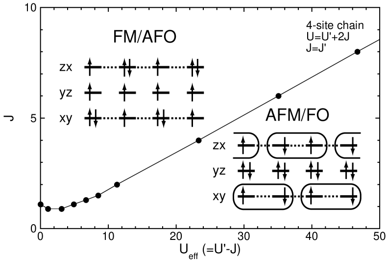
Figure 1: Ground-state phase diagram for the 4-site chain. Insets indicate schematic views for electron configurations in the AFM and FM phases. Oval enclosures represent the spin singlet pair for the VBS picture.

From the above discussion on the electron configuration, it is useful to consider the effective model in the strong-coupling region to clarify ground-state properties. For the AFM phase, the effective model is given by

$$H_{\rm AFM}=J_{\rm AFM}\sum_{i}({\bf S}_{i}\cdot{\bf S}_{i+1}-1),$$ (2)

where ${\bf S}_{i}$ indicates the $S$=1 operator and the AFM coupling $J_{\rm AFM}$ is expressed as $J_{\rm AFM}$=$2t^{2}/(U+J)$. On the other hand, the effective model in the FM phase is given by the $T$=1/2 AFO Heisenberg model

$$H_{\rm FM}=2J_{\rm FM}\sum_{i}({\bf T}_{i}\cdot{\bf T}_{i+1}-1/4),$$ (3)

with $J_{\rm FM}$=$2t^{2}/U_{\rm eff}$. We define pseudo-spin operator as ${\bf T}_{i}$=$(1/2)\sum_{\gamma,\gamma^{\prime},\sigma}d_{i\gamma\sigma}^{{\dagger}}\bm{\sigma}_{\gamma\gamma^{\prime}}d_{i\gamma^{\prime}\sigma}$, where $\bm{\sigma}$=$(\sigma_{x},\sigma_{y},\sigma_{z})$ are Pauli matrices and the summation for $\gamma$ and $\gamma^{\prime}$ is taken for $xy$ and $zx$ orbitals. Here we arrive at the following interesting conclusion: The AFM phase of the $t_{\rm 2g}$-orbital degenerate Hubbard model is the $gapped$ Haldane phase, well described by the spin $S$=1 AFM Heisenberg model $H_{\rm AFM}$. On the other hand, the FM phase is described by the pseudo-spin $T$=1/2 AFO Heisenberg model $H_{\rm FM}$ with the $gapless$ excitation.

We believe that the characteristics grasped within the small 4-site chain are physically meaningful, but it is highly required to confirm them without finite size effects. In order to consider numerically the problem in the thermodynamic limit, we employ the infinite-system DMRG method with open boundary condition.White Note that one site consists of three $t_{\rm 2g}$ orbitals and the number of bases is 64 for one site, indicating that the matrix size becomes very large. In the present calculation, the number of states kept for each block $m$ is up to $m$=160 and the truncation error is estimated as $10^{-5}$ at most.

In Fig. 2, the ground-state energy is plotted for $S_{\rm tot}^{z}$=0 and $N$ (the number of sites, i.e., the maximally polarized state). Here we fix $J$=6 to consider the strong-coupling region. Note that the energy is shifted by the constant of on-site Coulomb interactions $5U^{\prime}+U-3J$ for comparison with the effective model. In the AFM phase, the lowest-energy state is characterized by $S_{\rm tot}^{z}$=0 (solid circle), which is in agreement with the exact energy of $H_{\rm AFM}$ (dashed curve).note1 On the other hand, the energies for $S_{\rm tot}^{z}$=0 and $N$ are degenerated in the FM phase. The DMRG results (open circle) are compared with the exact energy of $H_{\rm FM}$ (solid curve).note2 The agreement is fairly well, except for a little discrepancy for small $U_{\rm eff}$, since the strong-coupling limit is appropriate for large $U_{\rm eff}$. Therefore, we conclude that the ground-state energy is well reproduced by the effective model in the strong-coupling region. Note that the phase transition takes place at a critical point $U_{\rm c}$$\simeq$33, which is similar to the value of the 4-site chain $U_{\rm c}(N$=$4)$$\simeq$35.

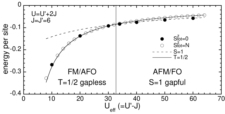
Figure 2: Ground-state energy per site as a function of $U_{\rm eff}$ for $J$=6 in the thermodynamic limit. Note that the origin of the energy is shifted (see the maintext). Dashed and solid curves denote exact ground-state energies for the $S$=1 AFM and $T$=1/2 AFO Heisenberg chains, respectively.

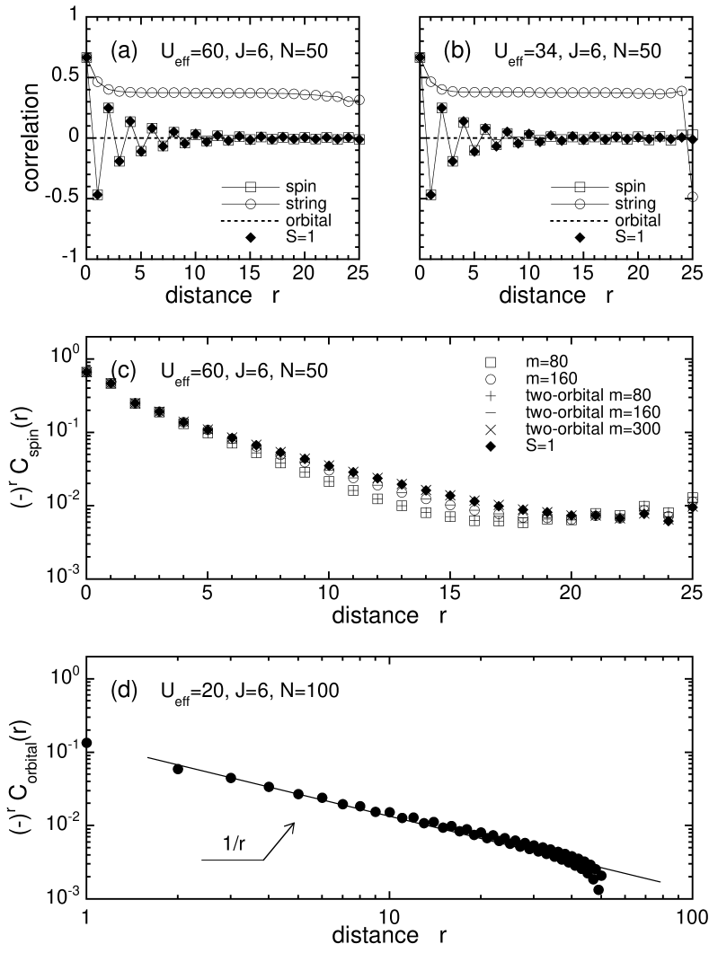
Figure 3: (a) Spin, string, and orbital correlation functions measured from the center of the chain for the AFM state. Here $r$ denotes the distance from the center position. Solid diamonds denote the spin correlation function of $H_{\rm AFM}$. (b) Correlation functions for $U_{\rm eff}$=34. (c) The linear-log plot of the spin correlation function in Fig. 3(a) and the two-orbital model. (d) The log-log plot of the orbital correlation function for the FM state.

In order to verify that ground-state properties are described by the effective model from the microscopic viewpoint, it is quite important to investigate correlation functions. For the AFM state, we evaluate the spin correlation function, $C_{\rm spin}(j,k)$=$\langle S_{j}^{z}S_{k}^{z}\rangle$, the string correlation function,Nijs-Rommelse $C_{\rm string}(j,k)$=$\langle S_{j}^{z}\exp[i\pi\sum_{l=j}^{k-1}S_{l}^{z}]S_{k}^{z}\rangle$, and the orbital correlation function, $C_{\rm orbital}(j,k)$=$\langle T_{j}^{z}T_{k}^{z}\rangle$. Here $\langle\cdots\rangle$ indicates the average using the ground-state wavefunction. In Fig. 3(a), we show correlation functions for $U_{\rm eff}$=60. We also depict $C_{\rm spin}$ of $H_{\rm AFM}$ obtained by the quantum Monte Carlo (QMC) method with the loop algorithm.note-qmc We observe that $C_{\rm spin}$ rapidly decays in accordance with the QMC results and the string long-range order exists, indicating that the characteristics of $H_{\rm AFM}$ are reproduced and the system has the gapful nature with respect to the spin. Note that the orbital has no effect on the low-lying excitation due to the localization of $yz$ orbital, as shown by dashed line in Fig. 3(a). For $U_{\rm eff}$=34 (near the phase boundary), the behavior of correlation functions in the bulk is also described by $H_{\rm AFM}$, as shown in Fig. 3(b). Note that anomaly due to open boundary condition appears just at the chain edge, since an orbital singlet dimer state with FM spin structure is stabilized to gain energy locally at the chain edge.

In Fig. 3(c), we show $C_{\rm spin}$ in the linear-log scale, indicating evidence of the exponential decay, although there is slight deviation from that of the QMC result for $H_{\rm AFM}$. In the DMRG calculation for $H$, the truncation error is about 10^-7 for $m$=160 and the energy is evaluated in this accuracy. However, in order to evaluate $C_{\rm spin}$ in the same accuracy, it is necessary to increase $m$ further and check the convergence with respect to $m$. Unfortunately, it is quite difficult to perform such tasks due to the large matrix size. Instead, here we introduce a two-orbital Hubbard model composed of $xy$ and $zx$ orbitals, in order to reduce the matrix dimension effectively. When we compare the results of the effective two-orbital model and the original Hamiltonian for $m$=80 and 160, good agreement is obtained as shown in Fig. 3(c), indicating that the two-orbital model well reproduces ground-state properties of $H$ in the AFM region. Further increasing $m$ up to $m$=300 in the two-orbital model to improve the precision of the finite-system DMRG method, we confirm that $C_{\rm spin}$ of the two-orbital model converges to that of $H_{\rm AFM}$. Then, it is highly believed that the same convergence should be observed for the original $t_{\rm 2g}$-orbital model.

For the FM state, we evaluate $C_{\rm orbital}$. Note that $C_{\rm spin}$ is constant depending on $S_{\rm tot}^{z}$ in the maximally spin-polarized FM phase. In Fig. 3(d), we observe the power-law decay of $C_{\rm orbital}$, which is characteristic of the half-odd-integer-spin chain. Namely, the system is described by $H_{\rm FM}$ and quantum fluctuation with respect to the orbital gives the gapless excitation. Further, the spin-wave excitation presents due to FM ordering and thus, both spin- and orbital-wave excitations are expected to exist.

Now we discuss relevance of our results to actual systems. We have performed the DMRG calculations for large value of $J$=6, to discuss the behavior in the strong-coupling region. However, we have confirmed that for the small 4-site chain, spin and orbital structures show characteristic behavior in each phase even in the weak-coupling region with small $U_{\rm eff}$ and $J$. In addition, as mentioned above, the phase boundary for $J$=6 is almost the same as that obtained in the 4-site chain. Namely, it is expected that the phase diagram in Fig. 1 does not change so much even in the thermodynamic limit, although the AFM region may somewhat extend. If we assume $t$=0.4eV, $U$=7eV, and $J$=1eV as typical values for transition metal oxides,Dagotto-review we obtain $U_{\rm eff}/t$=10 and $J/t$=2, where the system is expected to be near the phase boundary. Thus, the transition from gapful AFM to gapless FM phases may be controlled by chemical pressure.

In addition to the control of the Coulomb interactions or the bandwidth, it is possible that the magnetic field induces ferromagnetism in the Haldane system.comment The system is in the singlet ground state below a critical field due to the Haldane gap, indicating that magnetic moment is suppressed. At the critical field, finite value of magnetic moment begins to grow. Note that in actual systems, spin-canted AFM phase occurs. Increasing further the magnetic field, the saturated FM state should occur, when we apply a high magnetic field corresponding to 4$J_{\rm AFM}$.note3 For instance, this value may be estimated as 200 Teslas for LiVGe₂O₆, but smaller in other Haldane systems. The gapless excitation with respect to the orbital is expected to be observed in a similar way that the orbital-wave excitation has been revealed by Raman scattering measurements in LaMnO₃.orbiton

In summary, ground-state properties of the $t_{\rm 2g}$-orbital degenerate Hubbard model have been investigated in order to clarify effects of orbital degeneracy in the spin $S$=1 Haldane system. In the AFM phase, the spin $S$=1 AFM Heisenberg model is reproduced, while in the FM phase, the system is described by the pseudo-spin $T$=1/2 AFO Heisenberg model. Thus, we conclude that the low-energy physics is drastically changed due to the interplay of spin and orbital degrees of freedom. In particular, the gapless orbital excitation exists in the FM state. It may be interesting to observe such orbital excitation in the Haldane system under the high magnetic field.

The authors thank K. Kakurai and K. Yoshimura for discussions and comments. One of the authors (T.H.) is supported by a Grant-in-Aid from the Ministry of Education, Culture, Sports, Science and Technology of Japan.

References

- (1) F. D. M. Haldane, Phys. Lett. 93A, 464 (1983); Phys. Rev. Lett. 50, 1153 (1983).
- (2) I. Affleck et al., Phys. Rev. Lett. 59, 799 (1987); Commun. Math. Phys. 115, 477 (1988).
- (3) T. Kennedy and H. Tasaki, Phys. Rev. B 45, 304 (1992); Commun. Math. Phys. 147, 431 (1992).
- (4) M. Oshikawa, J. Phys.: Condens. Matter 4, 7469 (1992).
- (5) M. P. Nightingale and H. W. J. Blöte, Phys. Rev. B 33, 659 (1986).
- (6) T. Sakai and M. Takahashi, Phys. Rev. B 42, 1090 (1990).
- (7) S. R. White and D. A. Huse, Phys. Rev. B 48, 3844 (1993).
- (8) J. P. Renard et al., Europhys. Lett. 3, 945 (1987).
- (9) K. Katsumata et al., Phys. Rev. Lett. 63, 86 (1989).
- (10) M. Hagiwara et al., Phys. Rev. Lett. 65, 3181 (1990).
- (11) P. Millet et al., Phys. Rev. Lett. 83, 4176 (1999).
- (12) J. Lou et al., Phys. Rev. Lett. 85, 2380 (2000).
- (13) F. Milla and F. C. Zhang, Eur. Phys. J. B 16, 7 (2000).
- (14) P. Vonlanthen et al., Phys. Rev. B 65, 214413 (2002).
- (15) J. Sirker and G. Khaliullin, Phys. Rev. B 67, 100408(R) (2003) and references therein.
- (16) S. R. White, Phys. Rev. Lett. 69, 2863 (1992); Phys. Rev. B 48, 10345 (1993).
- (17) For the effective model (2), we adopt =1.4015, obtained by the quantum Monte Carlo simulation.
- (18) For the effective model (3), the Bethe-Hulthén solution, =+1/4, is available. See H. A.Bethe, Z. Physik 71, 205 (1931); L. Hulthén, Arkiv Mat. Astron. Fysik 26A, 1 (1938).
- (19) M. den Nijs and K. Rommelse, Phys. Rev. B 40, 4709 (1989).
- (20) H. G. Evertz, Adv. Phys. 52, 1 (2003). Here we have performed QMC simulations for the open-boundary chain at sufficiently low temperature /=0.01, and the data are sampled within the subspace of =0.
- (21) See, e.g., E. Dagotto et al., Phys. Rep. 344, 1 (2001).
- (22) Note that this is the direct transition between the AFM and FM phases. Here we emphasize that -orbital degeneracy could remain effective in the FM phase of the Haldane system, leading to gapless excitation.
- (23) The saturation field is given by the energy difference between the fully polarized states with the total spin = and 1, i.e., /==4.
- (24) E. Saitoh et al., Nature 410, 180 (2001).