Non-Hermitian Luttinger liquids and flux line pinning in planar superconductors

Abstract

As a model of thermally excited flux liquids connected by a weak link, we study the effect of a single line defect on vortex filaments oriented parallel to the surface of a thin planar superconductor. This problem can be mapped onto the physics of a Luttinger liquid of interacting bosons in 1 spatial dimension with a point impurity. When the applied magnetic field is tilted relative to the line defect, the corresponding quantum boson Hamiltonian is non-Hermitian. We analyze this problem using a combination of analytic and numerical (density matrix renormalization group) methods, uncovering a delicate interplay between enhancement of pinning due to Luttinger liquid effects and depinning due to the tilted magnetic field. Interactions allow a single columnar defect to be very effective in suppressing vortex tilt when the Luttinger liquid parameter $g\leq 1.$

I Introduction

The past fifteen years have seen much work on the statistical mechanics and dynamics of thermally excited vortices in Type II high temperature superconductors.bishop92 ; blatter94 ; tauber97 ; nattermann00 The competition between interactions, pinning and thermal fluctuations gives rise to a wide range of novel phenomena, including a first order melting transition of the Abrikosov flux lattice into an entangled liquid of vortex filaments,nelson88 a proposal for a highly disordered vortex glass dominated by point pinning,fisher89a a theory of a Bose glass phase with vortices strongly pinned to columnar defects,nelson92 and a distinct Bragg glass where point disorder converts Bragg peaks associated with crystalline order into power law singularities.giamarchi94

Much progress can be made on these problems using a classical continuum elastic theory.blatter94 An alternative approach, useful for treating parallel columnar defects, is to regard each vortex as an imaginary-time world line of a boson in a Feynman path integral, corresponding to a quantum theory of interacting bosons.nelson88 ; fisher89b Here the imaginary time direction $\tau$ is parallel to the columnar defects. A hydrodynamic treatment of this quantum model leads naturally to the same continuum elastic theory, where the classical free energy is now a classical action. If the direction of the external magnetic field does not coincide with that of columnar defects, it is convenient to separate the transverse component of the field $H_{\bot}$ from the parallel component $H_{||}$ along ${\bf{\hat{\tau}}}.$ When $H_{\bot}<<H_{||}$, the transverse component $H_{\bot}$ plays the role of a constant imaginary vector potential for the bosons.nelson92 ; hatano97 The corresponding fictitious quantum Hamiltonian is non-Hermitian, with new and interesting properties. Stimulated by vortex physics, there has been considerable work on non-Hermitian models of non-interacting bosons in a constant imaginary vector potential, $h\propto H_{\bot}$, and a disordered site-diagonal pinning.efetov97 ; brouwer97 ; mudry98 Since the Hamiltonian is non-Hermitian, the energy eigenvalues can be either real or complex. As discussed in [hatano97, ], all states with complex eigenvalues are extended, whereas those with real eigenvalues are usually localized.

Less is known about non-Hermitian models with interactions.nelson92 ; hatano97 A disordered array of parallel columnar defects leads to a strongly pinned low temperature Bose glass phase. For $h$ less than a critical value $h_{c}$, this phase exhibits a “transverse Meissner effect”, such that the vortex filaments remain pinned to the columns even though the external field is tilted away from the column direction. Although the transverse Meissner effect has now been observed in many high $T_{c}$ superconductors with correlated disorder, recent measurementsphuoc02 of the flux flow resistivity for $h_{\bot}\gtrsim h_{c}$ disagree with a simple theory which assume that vortices tilt from column to column via kink excitations.hwa93 Interactions combined with vortex pinning for a periodic array of columnar defects were studied using a non-Hermitian boson Hubbard model in [lehrer98, ]. Here, tilting the field drives a transition out of a low temperature “Mott insulator” phase (periodic array of vortices attached to the columns with an energy gap) into a “superfluid” phase, i.e., an entangled flux liquid. The corresponding non-Hermitian boson Hubbard model with site-diagonal disorder was studied in $(1+1)$-dimensions using a Hartree-Bogoliubov approximation in [kim01, ].

In this paper, we study the effect of a single columnar pin on the statistical mechanics of thermally fluctuating vortex lines confined in a thin, superconducting slab. (See Fig. (1).) The external field can tilt away from the direction of the column, leading to statistical physics controlled by a non-Hermitian quantum Hamiltonian. As discussed below, the physics is equivalent to a Luttinger liquid of interacting bosons with a point impurity. Tilting the field introduces a constant imaginary vector potential.

Figure 1: Vortices with a single columnar pin (heavy vertical line) and parallel magnetic field with displacement field $u(x,\tau)$ defined.

This problem is interesting for a number of reasons. If the average spacing between columnar defects is $d$, this is the regime $H>>B_{\phi}=\phi_{0}/d^{2}$ where $B_{\phi}$ is the “matching field” and $\phi_{0}\approx 2.07\times 10^{-7}{\rm G\,cm^{2}}$ is the flux quantum. As emphasized by Radzihovsky,radzihovsky95 the large number of “interstitial” vortices between columnar defects could be locally crystalline or melted into a flux liquid. A third possibility is vortices in an immediate “supersolid” phase, which is both crystalline but nevertheless entangled, due to a finite concentration of line-like vacancy or interstitial defects.frey94 By studying the response to a single columnar pin we can better understand the response in these phases to a dilute concentration of columnar defects. A dilute concentration of twin planes, a common occurance in bulk samples of YBCO, provides a related example of correlated pinning.

We examine here a similar regime in $(1+1)$- dimensions, when only a single columnar pin is present. The feasibility of studying vortex physics in samples which are effectively $(1+1)$-dimensional was demonstrated by Bollé et. albolle99 , who used micromechanical oscillators to track the entry of quantized vortex filaments near $H_{c1}$ in a thin sample of the low $T_{c}$ superconductor ${\rm NbSe_{2}}$. The observed behavior could be described in the framework of interacting vortex lines in a $(1+1)$-dimensional random potential representing the effects of point disorder.

Similar experiments might be possible on thin high - $T_{c}$ platelet samples, with temperatures high enough to allow vortex interactions to screen out the effect of the point disorder. The effect of a single columnar pin might be mimicked by gouging a long straight scratch or notch on one side of a thin sample.zeldov A $(1+1)$ dimensional array of flux lines could be created by a field $\vec{H}$, approximately parallel to the notch, and strong enough to insert a single layer of flux lines into a sample with a thickness given roughly by the London penetration depth. As discussed below, $(1+1)$–dimensional arrays of vortex lines show algebraic decay of both translational order and the boson order parameter. Thus, experiments and theory on this $(1+1)$–dimensional problem might give some insight into the effect of a dilute concentration of columnar pins on a supersolid phase in $(2+1)$-dimensions. Because of the long range correlations, a single columnar defect can have a large effect on the flux liquid, similar to the screening cloud surrounding a Kondo impurity in a metal.

A related problem in $(2+1)$-dimensions concerns the effect of a single twin plane or grain boundary on vortex matter. A dense array of such planes parallel to the field direction leads to a Bose glass phase at low temperatures and a flux liquid at high temperatures.nelson92 A single such plane should have an interesting influence on the vortex matter which surrounds it. Consider the effect of a small tilt on the vortex configurations. The “motion” of the tilted vortex configurations across the twin plane is an imaginary time version of particle transport across a Josephson junction. The “transport” process is likely to be quite different, depending on whether the surrounding vortex matter is in a flux liquid, vortex crystal or supersolid phase. A single planar defect in $(2+1)$-dimensions would also have a strong effect on the flux flow resistivity in response to a current parallel to the plane leading to a Lorentz force which is approximately perpendicular to it. Motion of the Bragg planes of the Abrikosov flux lattice across such a defect is reminiscent of transport in materials with charge density waves.lee

The single defect, (1+1) dimensional physics problem is very tractible using the continuum elastic field theory approach. Its quantum hydrodynamic formulation corresponds to a single component “Luttinger liquid”.Haldane The resulting field theory, when the field is parallel to the defect, is identical to one studied earlierKane in the context of interacting one-dimensional (spinless) fermions with a point defect and of a defect in an S=1/2 Heisenberg antiferromagnetic chain.Eggert We directly apply these results to the present situation. These results depend crucially on a dimensionless parameter, $g$ which controls all critical properties of the model.Kane For instance the density correlations (with no defects) exhibit power law decay with an exponent $\eta=2g$. For interacting fermions $g<1$ corresponds to repulsive interactions and $g>1$ attractive interactions. In the bosonic case the dependence of $g$ on microscopic parameters is more subtle, as we discuss. When $g>1$ a defect is an irrelevant perturbation at long length scales, in the renormalization group (RG) sense, whereas when $g<1$ it is relevant, effectively flowing to infinity in the long wavelength limit. As was first suggested by DeGennes,deGennes in the dilute limit our vortex problem is equivalent to free fermions, $g=1$ .deGennes ; Pokrovskii ; Coppersmith ; Haldane We show that a transverse magnetic field defines a characteristic length scale, $\propto 1/h$, which acts as an infrared cut off scale in the renormalization group flow equations. Thus even when $g<1$, a defect is ultimately an irrelevant perturbation at sufficiently long length scales.

We also study a tight-binding version of the non-Hermitian 1D quantum model using the Density Matrix Renormalization Group (DMRG) method generalized to treat non-Hermitian Hamiltonians. This powerful method provides valuable checks on our RG arguments and more detailed information about the model.

We focus on the vortex density (i.e. magnetic field) oscillations set up by a single columnar pin as well as on the transverse Meissner effect. These correspond, respectively, to generalized Friedel oscillations and an imaginary current in the quantum problem. While these Friedel oscillations have power-law decay for a parallel field, they decay exponentially when $h\neq 0$. The imaginary current can be expressed in terms of a “pinning number”, $N_{p}$, which measures how many bosons are stuck in the vicinity of the defect at any given “time”. We find that $N_{p}$ can diverge as $h\to 0$, with different critical behavior in the cases $g\leq 1$ and $g>1$.

A real sample would always contains some density of point defects in addition to one or more line defect. We show that any finite density of point defects alters the critical behavior associated with the line defect at sufficiently large length scales. Thus to observe the critical behavior caused by a single line defect it will be neccessary to have sufficiently clean samples.

In the next section we briefly review the classical continuum elastic theory of fluctuating lines and the approach based on mapping into a quantum model. We also discuss the value of $g$, showing that it goes to $1$ at low densities and $0$ at higher densities. We note that $g$ need not be a monotonic function of density for vortex arrays. It is possible that $g$ passes through unity at some finite density as well. In Sec. III we study the $g=1$ case, which occurs in the dilute limit, by exploiting the correspondence to non-interacting fermions. In Sec. IV we study general values of $g$ using renormalization group and numerical methods, extending earlier resultsKane ; Eggert to the non-Hermitian case. Sec. V contains a discussion of point defects. Sec. VI contains our conclusions.

Appendix A derives a result for interacting bosons in one dimension of general applicability. While it is well known that $g\to 1$ in the dilute limit, corresponding to free fermions, we study the leading correction to this behavior at small finite density, $n_{0}$. We find that the result can be conveniently expressed in terms of the even channel scattering length, $a$. This quantity is determined entirely from the 2-body scattering problem, and is straightforward to calculate for any particular 2-body interaction. Our new general result is:

$$g\approx 1-2an_{0}+O(n_{0}^{2}).$$ (1)

The scattering length, $a$, can be positive or negative depending on the details of the interactions, even though they are always assumed to be purely repulsive.

Appendix B discusses determination of the value of $g$ for our tight-binding model. In Appendix C we present results on the correlation function of the boson creation operator which is useful in confirming the RG picture regarding the relevance or irrelevance of a defect. Appendix D discusses the difference in ground state energy for periodic versus anti-periodic boundary conditions, another useful diagnostic for relevance or irrelevance of a defect. Appendix E contains some estimates of the effects of point disorder. Appendix F points out the connection between our model and one which has recently attracted attention from the string theory community.

A brief summary of these results appeared earlier.Hofstetter

II Classical and quantum formulations of interacting flux lines in (1+1) dimensions

Following, e.g., [hwa93, ] we consider a model free energy $F$ for $N$ flux lines in an extreme type II superconducting sample of thickness $L_{\tau}$ in the $\tau$ direction in the presence of a single columnar defect aligned in the $\tau$ direction and located at $x=0$:

$$F=\int^{L_{\tau}}_{0}d\tau\left\{\sum_{i=1}^{N}\left[{{\tilde{\epsilon}_{1}}\over 2}\left[{{dx_{i}(\tau)}\over{d\tau}}\right]^{2}-\epsilon_{d}\cdot\delta[x_{i}(\tau)]-{{\phi_{0}H_{\perp}}\over{4\pi}}\cdot{{dx_{i}(\tau)}\over{d\tau}}\right]+{1\over 2}\sum_{i\neq j}V_{\hbox{int}}[|x_{i}(\tau)-x_{j}(\tau)|]\right\}$$ (2)

where $x_{i}(\tau)$ denotes the trajectory of the $i^{th}$ vortex line, $V_{\hbox{int}}(x)$ is the repulsive interaction potential between flux lines, which can be taken to be local in $\tau$. We don’t expect this locality assumption to qualitatively change the long distance physics in the dilute limit. The coupling $\epsilon_{d}$ measures the (attractive) interaction between a flux line and the columnar defect. The tilt modulus, in the dilute limit, $n_{0}\lambda<<1$, where $n_{0}$ is the vortex density and $\lambda$ is the penetration depth, (i.e. $H\gtrsim H_{c1}$), for a planar sample which is invariant under rotations in the plane is

$$\tilde{\epsilon}_{1}=\left({{\phi_{0}}\over{4\pi\lambda}}\right)^{2}\ln\>\kappa,$$ (3)

where $\kappa=\lambda/\xi$ is the ratio of the London penetration depth $\lambda$ and the coherence length $\xi$. The canonical partition function for a system of $N$ lines is given by the Boltzmann integral:

$$Z={1\over N!}\Pi^{N}_{i=1}\int{\mathcal{D}}[x_{j}(z)]\>e^{-F[\{x_{i}(z)\}]/T},$$ (4)

where we have set $k_{B}=1$.

From here it is possible to pass directly to a continuum elastic formulation of this model or else to use a quantum description where we regard $x_{j}(\tau)$ as the trajectory of a particle and the classical Boltzmann sum as a Feynman path integral. We pursue the first direction in sub-section A and the second in sub-section B. Upon using a quantum hydrodynamics approximation to the quantum model we obtain the same continuum field theory. This field theory contains some parameters which we estimate, starting from the underlying vortex model, in sub-section C.

II.1 Classical continuum elastic theory

It is very convenient to pass to a continuum approximation using a coarse-grained displacement field, $u(x,\tau)$, like that used to describe a two-dimensional smectic liquid crystal in an external field.Domb A standard way of doing this is to write the trajectory of the $j^{\hbox{th}}$ vortex as:

$$x_{j}(\tau)=ja_{0}+u_{j}(\tau),$$ (5)

(see Fig. 1a) where $a_{0}=n_{0}^{-1}$ is the average vortex spacing in the $x$-direction and define $u(x,\tau)$ at the “equilibrium” positions of the vortices by:

$$u(ja_{0},\tau)=u_{j}(\tau).$$ (6)

This identification implies that the coarse grained density is:

$$n(x,\tau)\approx n_{0}\left[1-{\partial u\over\partial x}\right].$$ (7)

While this definition of $u$ is standard also in higher dimensions, there is another way of defining it, special to 1 dimension which has certain advantages but is essentially equivalent. We first define a field $A(x,\tau)$ by the requirement that the position of the $j^{\hbox{th}}$ vortex along a constant $\tau$ slice is the point $x$ where $A(x,\tau)=j$. Thus $A(x,\tau)$ can be taken to be a smooth monotonic function of $x$ varying from $0$ to $N$ where $N$ is the number of vortices. [An arbitrary smooth interpolation of $A$ can be chosen between the points where it is integer-valued.] It thus follows that the density is:

$$n(x,\tau)\equiv\sum_{j=1}^{N}\delta[x-x_{j}(\tau)]={\partial\over\partial x}\sum_{j=-\infty}^{\infty}\theta[A(x,\tau)-j],$$ (8)

where $\theta(x)$ is the step function. ($\theta(x)=0$ for $x<0$ and $\theta(x)=1$ for $x>0$.) Note that this definition implies that the number of vortex lines, along a constant $\tau$ slice, between $x_{1}$ and $x_{2}$ is:

$$\int_{x_{1}}^{x_{2}}n(x,\tau)dx=[A(x_{2},\tau)]-[A(x_{1},\tau)],$$ (9)

where $[A]$ denotes the integer part. On the other hand, Eqs. (5) and (7) imply that this quantity is:

$$\int_{x_{1}}^{x_{2}}n(x,\tau)dx\approx n_{0}\{(x_{2}-x_{1})-[u(x_{1},\tau)-u(x_{2},\tau)]\}.$$ (10)

Thus we write:

$$A(x,\tau)=n_{0}[x-u(x,\tau)],$$ (11)

and see that these two definitions of $u(x,\tau)$ are equivalent in a coarse-grained limit.

Upon using the Poisson summation formula, the density in Eq. (8)can be written:

$$n(x,\tau)={\partial A\over\partial x}\sum_{j=-\infty}^{\infty}\delta[A(x,\tau)-j]={\partial A\over\partial x}\sum_{m=-\infty}^{\infty}e^{2\pi imA(x,\tau)}.$$ (12)

When reexpressed in terms of $u$ this identity becomes:

$$n(x,\tau)=n_{0}\left[1-{\partial u\over\partial x}\right]\sum_{m=-\infty}^{\infty}e^{iG_{m}x}e^{-iG_{m}u(x,\tau)}.$$ (13)

Here the reciprocal lattice vectors, $\{G_{m}\}$ are

$$G_{m}=2\pi m/a_{0},\ \ m=0,\pm 1.\ldots$$ (14)

We neglect the columnar pin for the moment and use the standard continuum elastic energy for a set of tilted vortex lines in (1+1)–dimensions, namelyblatter94 ; fisher89a ; hwa93

$$F_{0}=\int dxd\tau\left[\frac{1}{2}c_{44}\left(\partial_{\tau}u\right)^{2}+\frac{1}{2}c_{11}\left(\partial_{x}u\right)^{2}-(n_{0}\phi_{0}H_{\perp}/4\pi)\left(\partial_{\tau}u\right)\right]$$ (15)

where $c_{11}$ and $c_{44}$ are the compressional and tilt moduli respectively. We see from Eqs. (2) and (5) that:

$$c_{44}\approx n_{0}\tilde{\epsilon}_{1}.$$ (16)

Although the $T=0$ value of $c_{11}$ is determined by vortex interactions as

$$c_{11}\approx n_{0}^{2}\int dyV_{\hbox{int}}(y),$$ (17)

thermal fluctuations and confinement entropy of interacting vortex lines lead to a value,Coppersmith

$$c_{11}\propto T^{2}n_{0}^{3}/\tilde{\epsilon}_{1},$$ (18)

in the limit $n_{0}\to 0$, where the dimensionless constant of proportionality is independent of the vortex interactions. The shear elastic constant $c_{66}$, necessary to describe a triangular Abrikosov flux lattice in (2+1)–dimensions, is absent. Elastic moduli such as $c_{11}$ and $c_{44}$ can be nonlocal (i.e., wavevector dependent in Fourier-spaceblatter94 ), but for the large distance physics of interest to us here, we can take them to be constants, equal to their values on scales much larger than the particle spacing or the range of the interaction.

Including the columnar pin simply adds a term to F:

$$F\to F-\epsilon_{d}\int d\tau n(0,\tau).$$ (19)

We can include this in our elastic free energy by using Eq. (13) to express $n(0,\tau)$. Many long wavelength properties of the vortex-pin system can be studied using this continuum free energy. However, for some purposes it is convenient to use the quantum mechanical formulation of the model, outlined in the next sub-section.

We note that the elastic continuum free energy of Eq. (15), with its adjustable constants $c_{\hbox{44}}$ and $c_{\hbox{11}}$, modified as appropriate to account for point and/or columnar defects, is expected to give a valid description of the long distance physics of the vortex lattice for essentially arbitrary vortex densities. On the other hand, the simple free energy of Eq. (2) is only valid at low vortex densities, $n_{0}<\lambda^{-1}$, corresponding to fields not to far above $H_{c1}$. At higher fields nonlocal couplings are required to capture the physics at all length scales. Consequently, the estimate of $c_{44}$ in Eq. (16) is only expected to be valid at low densities.

II.2 Quantum formulation

Let us return to the original discrete formulation of our free energy, Eq. (2). We may regard $x_{j}(\tau)$, $j=1,2,3,\ldots N$ as the trajectories of $N$ particles. To describe a physical sample containing vortices, the Boltzmann sum in Eq. (4) could be done by first holding the entry and exit points of the $N$ vortices at the top and bottom of the sample fixed. The Boltzmann sum includes summing over all permutations of which vortex $i$, enters and exits at each of the prescribed entry and exit points. The $1/N!$ factor is then neccesary to avoid over-counting. This expression can readily be seen to be the Feynman path integral for a density matrix of a system of $N$ bosons.nelson88 Eq. (4) can be rewritten in terms of the imaginary-time evolution operator $e^{-L_{\tau}{\hat{H}}/\hbar}$ as

$$Z=\left<\psi^{f}|e^{-L_{\tau}{\hat{H}}/\hbar}|\psi^{i}\right>,$$ (20)

where the bra and ket vectors are the initial and final states, respectively, obtained by summing over all entry and exit points. The quantum Hamiltonian $\hat{H}$ describes an ensemble of interacting bosons and is given by

$$\hat{H}=-{\hbar^{2}\over 2m}\int dx\psi^{\dagger}\left({d\over dx}-h\right)^{2}\psi+{1\over 2}\int dx\,dy\,\hat{n}(x)\,V(|x-y|)\,\hat{n}(y)-\epsilon_{0}\hat{n}(0).$$ (21)

where $\psi(x)$ is the bosonic annihilation operator and

$$\hat{n}(x)\equiv\psi^{\dagger}(x)\psi(x),$$ (22)

is the boson number density. To account for tilting of the external field away from the direction of the pin, an imaginary vector potential $ih$ has been included, thus making the Hamiltonian non-Hermitian. In the following we will set $\hbar=1$. We measure time, $\tau$, as well as position, $x$, in units of length. Thus various parameters in the quantum model have unusual dimensions.

Table 1: Correspondence between quantities in classical vortex line problem and quantum boson problem. $\mu$ is the boson chemical potential. $\hbar$ is Planck’s constant but $h$ is the transverse field. Although the dimensions of corresponding quantites do not match, they do upon forming physically relevant combinations such as $\hbar^{2}/2m\leftrightarrow T^{2}/2\tilde{\epsilon}_{1}$.

Vortex Lines	Bosons
$\tilde{\epsilon}_{1}$	$m$
$V_{\hbox{int}}(x)$	V(x)
$\epsilon_{d}$	$\epsilon_{0}$
$L_{\tau}$	$\beta\hbar$
$H_{||}w/{\phi_{0}}$	$n_{0}$
$\phi_{0}H_{||}/(4\pi)-\tilde{\epsilon}_{1}$	$\mu$
$\phi_{0}H_{\perp}/(4\pi)$	$h$
$T$	$\hbar$

In Table (1) we show the correspondences between various physical quantities in the classical vortex and quantum boson models. Here $n_{0}=a_{0}^{-1}$ is the average number of bosons per unit length in the one-dimensional (1D) quantum system and $w$ is the thickness of the slab.

For numerical simulations it is convenient to define a lattice regularization of the model (21):

$$\hat{H}=\sum_{i=0}^{L-1}\left[-t\left(b^{\dagger}_{i}b_{i+1}e^{-h}+b^{\dagger}_{i+1}b_{i}e^{h}\right)+{U\over 2}\hat{n}_{i}(\hat{n}_{i}-1)+V\hat{n}_{i}\hat{n}_{i+1}-\epsilon_{0}\hat{n}_{0}\right].$$ (23)

although this lattice has no physical meaning. Here $\hat{n}_{i}\equiv b^{\dagger}_{i}b_{i}$ denotes the boson density on lattice site $i$. The equivalence between (21) and (23) holds for low densities per lattice site $n_{0}<<1$. For numerical convenience, the Hilbert space is restricted so that there can only be 0, 1 or 2 bosons on each site. We normally impose periodic boundary conditions:

$$b_{L}\equiv b_{0}.$$ (24)

In the low density limit, small $h$ limit, Eq. (23) reduces to the continuum model (21) with:

$$t=1/2m.$$ (25)

To obtain a quantitative understanding of the analytical approximations used in this paper, and to determine numerically the Luttinger liquid parameter $g$, we have applied a non-hermitian generalization of the density matrix renormalization group (DMRG) algorithm to the tight-binding Hamiltonian (23). The DMRG methodWhite92 was originally invented to determine in a quasi-exact fashion numerically the properties (order parameters, correlations, structure functions) of the ground or low lying excited states of one-dimensional, strongly correlated quantum Hamiltonians, preferably with short-ranged interactions. In contrast to many other techniques, DMRG performance is typically enhanced by strong interactions. System sizes that can be studied for Heisenberg or Hubbard-type models reach up to the order of a thousand sites. A good introduction and overview of many of the original DMRG applications may be found in Ref. (Peschel99, ).

The key idea of DMRG is to grow iteratively, starting from some very small system size which can still be diagonalized exactly, a sequence of systems of linearly increasing size while carrying out reduced basis transformations at each growth step to keep the size of the underlying Hilbert space fixed. This reduced basis transformation is chosen such as to introduce the minimal error in the representation of the physical state of interest, most often the ground state. This is achieved by determining this state $|\psi\rangle$ by some large sparse matrix diagonalization algorithm, and partitioning the entire system into two blocks $A$, $B$ for which density matrices are derived by tracing out the states of the other block in the pure state projector, $\hat{\rho}_{A(B)}={\rm Tr}_{B(A)}|\psi\rangle\langle\psi|$. The eigenvalue spectra of the density matrices determine the new reduced bases for the system parts by choosing as new bases for the blocks a fixed number $m$ of eigenstates of the density matrices characterized by the largest eigenvalues.

This fundamental idea of the DMRG was generalized to renormalize not just quantum Hamiltonians, but also classical transfer matrices for statistical mechanics problems in two dimensionsNishino95 and quantum transfer matrices to study the thermodynamic properties of one-dimensional quantum systemsBursill96 , complementing the $T=0$ results of the original method. Carlon, Henkel and SchollwöckCarlon99 have generalized the DMRG method to renormalize strongly non-hermitian transition matrices that originate in a master equation formulation of reaction-diffusion problems. The steady-state behaviour of these systems can then be derived from the left and right eigenstates corresponding to the eigenvalue with the smallest real part which are thus the “ground state” pair of that problem. This DMRG variant can be directly applied to determining the ground state eigenfunction pair of a non-hermitian quantum mechanics problem.

The main numerical problem in the generalization of the DMRG to non-hermitian systems is given by the observation that non-hermitian diagonalization of large sparse matrices is much less stable than in the hermitian case. While eigenvalues can be obtained with satisfactory precision, eigenstates show small numerical inaccuracies that tend to accumulate during DMRG runs as these eigenstates are at the basis of the reduced basis transformations carried out in each DMRG step. In the unsymmetric Lanczos algorithm we have usedGolub96 , the origin of these inaccuracies is mainly due to the inevitable loss of the global biorthonormality of the sets of Lanczos ansatz states for right and left eigenstates. We have achieved good numerical stability by applying a selective, very time-efficient re(bi)orthogonalization procedure introduced by DayDay97 .

In determining the density matrices for the non-hermitian DMRG, there is a further arbitrariness: there are both symmetric and nonsymmetric density matrices, defined by partial traces, $\hat{\rho}_{symm}=(1/2){\rm Tr}(|\psi_{R}\rangle\langle\psi_{R}|+|\psi_{L}\rangle\langle\psi_{L}|)$ and $\hat{\rho}_{nonsymm}={\rm Tr}|\psi_{R}\rangle\langle\psi_{L}|$ respectively, where $\langle\psi_{L}|$ and $|\psi_{R}\rangle$ are the left and right eigenstates of interest for the total system. The reduced basis transformations derived from the two choices are not identical. There is no clear-cut preference in non-hermitian DMRG: In the case of the quantum transfer matrix DMRG, which also suffers from (weak) non-hermiticity, the unsymmetric choice was found to be superior in precisionNishino99 , whereas in another non-hermitian DMRG version, the stochastic transfer matrix DMRG, only the symmetric choice yields useful informationKemper01 ; Enss01 . Studies we have carried out for our problem of interest indicate that both approaches are feasible for high accuracy, but that numerical stability concerns favor the symmetric choice.

With these choices made, we have studied system sizes up to $L=256$ sites with up to $N=64$ bosons, the particle density being at or below a quarter. Up to $m=300$ states have been kept in the reduced Hilbert spaces and found to give effectively converged results for currents, energies, and local quantities such as particle densities. The low particle density, leading to a strong arbitrariness in the insertion of particles during system growth, and the presence of an impurity mandate the application of the so-called finite-size DMRG algorithm,White92 which has been applied up to 11 times to achieve converged results.

In applying DMRG to bosonic systems, the possibly divergent number of bosons per site has to be truncated algorithmically to some maximum number. As we are considering superconductors in the low flux line density limit, we fixed the maximum number of bosons per site to be 2. This constraint is consistent with average particle densities of no more than $0.25$; the validity of this truncation has been checked for selected parameter sets by increasing the maximum number of bosons per site. It should be mentioned that these findings are not at variance with the statement that in Luttinger liquids with $g<1$ impurities correspond to relevant perturbations and scale to infinity in effective field theories under renormalization group (RG) flow.Kane ; Eggert In the underlying lattice model, the resulting perfect pinning is effected by the generation of a very long-ranged effective local pinning potential whose strength decays only as a power law away from the impurity, but whose scale is essentially that of the original impurity.Meden02 Hence, we do not expect a particularly strong enhancement of the local boson density at the impurity site, as confirmed by our numerical results; in all runs, even at the impurity site, the boson density is well below 1 for all impurity strengths considered in this paper.

We now pass to a quantum hydrodynamic formulation of this model.Haldane We may express the boson density operator in terms of a quantum field, $u(x)$, using Eq. (13). In order to conform to more standard notation in the quantum literature, we replace the displacement field, $u(x,\tau)$, which has dimensions of length, with a dimensionless field, $\theta(x,\tau)$:

$$\theta(x,\tau)\equiv-n_{0}u(x,\tau).$$ (26)

Thus Eq. (13) for the density operator becomes:

$$\hat{n}(x)=\left(n_{0}+{d\theta\over dx}\right)\sum_{m=-\infty}^{\infty}e^{2\pi im[n_{0}x+\theta(x)]}.$$ (27)

We write the boson creation operator in the form:

$$\psi^{\dagger}(x)\propto\sqrt{n_{0}+{d\theta\over dx}}\sum_{m=-\infty}^{\infty}e^{2\pi im[n_{0}x+\theta(x)]}e^{i\phi(x)},$$ (28)

with, of course, the Hermitian conjugate expression for the operator, $\psi(x)$. Note that this formula is consistent with $\hat{n}=\psi^{\dagger}\psi$ using the fact that $\delta^{2}(x)\approx\Lambda\delta(x)$ where $\Lambda$ is an ultra-violet cut-off with dimensions of wave-vector. We have introduced another bosonic field, $\phi(x,t)$, which represents the phase of $\psi^{\dagger}$. We generally keep only the most relevant terms (in a renormalization group sense) in these expressions, writing:

$$\hat{n}(x) \approx n_{0}+{d\theta\over dx}+\hbox{constant}\times\cos\{2\pi[n_{0}x+\theta(x)]\}$$

$$\psi^{\dagger}(x) \propto \hbox{constant}\times e^{i\phi(x)}.$$ (29)

The $\theta$ and $\phi$ fields do not commute. In fact, in order to correctly reproduce the continuum commutation relations between $\hat{n}(x)$ and $\psi^{\dagger}(x)$, namely

$$[\hat{n}(x),\psi^{\dagger}(y)]=\delta(x-y)\psi^{\dagger}(x),$$ (30)

we require:

$$[d\theta(x)/dx,\phi(y)]=-i\delta(x-y).$$ (31)

Thus, we can identify:

$$d\theta/dx=\hat{\Pi},$$ (32)

as the momentum operator conjugate to $\phi$. Upon integrating Eq. (31) we obtain:

$$[\phi(x),\theta(y)]=(-i/2)\ \hbox{sgn}(x-y),$$ (33)

where sgn$(x)$ is the sign function, $\hbox{sgn}(x)=x/|x|$. Thus we see that $[d\phi/dx,\theta(y)]=-i\delta(x-y)$ and hence the conjugate momentum to $\theta$ is

$$\hat{\Pi}_{\theta}=d\phi/dx.$$ (34)

We may now write a long wavelength low energy approximation to the Hamiltonian of Eq. (21) (ignoring, for the moment, the tilt field and pinning potential) in terms of these phonon and phase variables. Keeping only terms of quadratic order in the fields and their derivatives, the Hamiltonian density less the chemical potential times the particle density may be written, for convenience, in terms of two new parameters, a phonon velocity $c$ and a dimensionless “Luttinger liquid parameter” $g$:

$$\hat{\cal H}_{\phi}(x)-\mu\hat{n}(x)={c\over 2}\left[{g\over\pi}\left({d\phi\over dx}\right)^{2}+{\pi\over g}\hat{\Pi}^{2}\right].$$ (35)

The first term comes from the kinetic energy in Eq. (21) implying that

$${cg\over\pi}={n_{0}\over m}.$$ (36)

The second term comes from the interaction term, which leads to:

$${c\pi\over g}\approx\int dxV(|x|).$$ (37)

Upon canonically transforming to the Lagrangian and then going to imaginary time: $\tau\equiv it$, we have:

$${\partial\phi\over\partial t}={\pi c\over g}\hat{\Pi},$$ (38)

and the imaginary time action

$$S_{\phi}=\int_{0}^{L}dx\int d\tau{\cal L}_{\phi}(x,\tau),$$ (39)

where the Lagrangian density is

$${\cal L}_{\phi}(x,\tau)={g\over 2\pi}\left[{1\over c}\left({\partial\phi(x,\tau)\over\partial\tau}\right)^{2}+c\left({\partial\phi(x,\tau)\over\partial x}\right)^{2}\right].$$ (40)

Alternatively, we may write $\hat{H}$ in terms of the phonon field, $\theta$. With the help of Eqs. (32) and (34) we see that the Hamiltonian density can also be written as:

$$\hat{\cal H}_{\theta}-\mu\hat{n}={c\over 2}\left[{g\over\pi}\hat{\Pi}_{\theta}^{2}+{\pi\over g}\left({d\theta\over dx}\right)^{2}\right].$$ (41)

Another canonical transformation gives:

$${\partial\theta\over\partial t}={gc\over\pi}\hat{\Pi}_{\theta}$$ (42)

and hence the action in terms of the $\theta$-field reads:

$$S_{\theta}=\int_{0}^{L}dx\int d\tau{\cal L}_{\theta}(x,\tau),$$ (43)

with

$${\cal L}_{\theta}(x,\tau)={\pi\over 2g}\left[{1\over c}\left({\partial\theta(x,\tau)\over\partial\tau}\right)^{2}+c\left({\partial\theta(x,\tau)\over\partial x}\right)^{2}\right].$$ (44)

Eq. (44) is, of course, just the result obtained from classical continuum elastic theory, Eq. (15), with:

$$g = {\pi Tn_{0}^{2}\over\sqrt{c_{11}c_{44}}}$$

$$c = \sqrt{c_{11}\over c_{44}}.$$ (45)

It is straightforward to add the imaginary vector potential, $h$, in the quantum hydrodynamic formulation of the model. We begin with the Hamiltonian of Eq. (21) and then rewrite the boson creation operator, $\psi^{\dagger}$ using Eq. (29). The modification of the Hamiltonian density in $\phi$-representation is:

$${\cal H}_{\phi}\to{\cal H}_{\phi}-{ihn_{0}\over m}{d\phi\over dx}-{h^{2}\over 2m}n_{0}.$$ (46)

We may alternatively calculate the extra term in the Lagrangian density in $\theta$ representation, using Eq. (34) and then canonically transformating from Hamiltonian to Lagrangian, giving:

$${\cal L}_{\theta}\to{\cal L}_{\theta}+h{\partial\theta\over\partial\tau}.$$ (47)

This is, of course, consistent with Eq. (15), using Table I and Eq. (26).

II.3 The Luttinger liquid parameter $g$:  its significance and numerical value

The quantity $g$ is an essential parameter which determines all critical properties of the model, with or without a pin or a transverse field. In this sub-section we indicate the significance of $g$ and estimate its value for the physical vortex problem in the limits of dense and dilute vortices.

From Eq. (44) we see that the density field, $\theta$, has the correlator:

$$<\theta(\tau,x)\theta(0,0)>\approx-{g\over 4\pi^{2}}\ln[c^{2}\tau^{2}+x^{2}]+\hbox{constant}$$ (48)

With the help of Eq. (29), we see that the density correlation function is given by:

$$<n(x,\tau)n(0,0)>\to n_{0}^{2}+{gc^{2}\over 2\pi^{2}}{c^{2}\tau^{2}-x^{2}\over(c^{2}\tau^{2}+x^{2})^{2}}+\sum_{m=1}^{\infty}{A_{m}\cos(2\pi n_{0}mx)\over[x^{2}+c^{2}\tau^{2}]^{gm^{2}}}+\ldots,$$ (49)

where the $A_{m}$’s are constants. Note that a conventional vortex lattice cannot form in our two-dimensional system, but we get instead quasi-long range vortex order with density oscillations spaced by the average inter-vortex separation, $a_{0}$. The Fourier transformed density-density correlation function, or structure function, $S(q_{x},q_{\tau})$, has algebraic singularities at the reciprocal lattice wave-vectors, $G_{m}\equiv 2\pi mn_{0}$:

$$S(q_{x},q_{\tau})\propto\frac{1}{\left[c^{2}(q_{x}-G_{m})^{2}+q_{\tau}^{2}\right]^{1-gm^{2}}}\ \ [\hbox{for}\ (q_{x},q_{\tau})\approx(G_{m},0)]$$ (50)

We see that $S(\vec{q})$ diverges at $q_{x}=\pm G_{1}$, $q_{\tau}=0$ whenever $g<1$. See Fig. (2).

We can use the results above to assess the effect of a single columnar defect on the vortex density within perturbation theory. To lowest order in the pinning strength $\epsilon_{d}$ we find

$$\delta n(x,\tau) = <n(x,\tau)>-n_{0}$$ (51)

$$= \epsilon_{d}\int d\tau^{\prime}C(x,\tau-\tau^{\prime}),$$

where

$$C(x-x^{\prime},\tau-\tau^{\prime})=<n(x,\tau)n(x^{\prime},\tau^{\prime})>_{0}-<n(x,\tau)>_{0}<n(x^{\prime},\tau^{\prime})>_{0}.$$ (52)

Here, $<\ >_{0}$ represents an average in an ensemble where both tilt and the defect are absent. When Eq. (51) is rewritten in Fourier space, the linear response to the perturbation induced by the columnar pin is determined by the structure function. For a system with spatial extent $L_{\tau}$ in the time direction, we have

$$\delta n(q_{x},q_{\tau})=\epsilon_{0}S(q_{x},0)\,L_{\tau}\delta_{q_{\tau},0}$$ (53)

The most singular response is at wave-vector $(q_{x},q_{\tau})=(\pm G_{1},0)$, i.e. for $m=1$ in Eq. (50). Thus the response diverges for $g<1$ suggesting that a single pin is a relevant perturbation for $g<1$ but is irrelevant for $g>1$. This conclusion will be modified by a transverse field or by point disorder as we will see in later sections. The leading perturbative result for the oscillating part of $\delta n(x)$ at long distances from the pin in real space is thus:

$$\delta n(x,\tau)\propto{\epsilon_{0}\cos(2\pi n_{0}x)\over|x|^{2g-1}}.$$ (54)

Figure 2: (a) Reciprocal lattice vectors $(G_{m},0)$ in the $(q_{x},q_{\tau})$–plane for $h=0$. The structure function describing vortex correlations in reciprocal space is singular at these points . The Fourier–transformed potential of a single attractive columnar defect is only nonzero on the heavy line along the $q_{x}$–axis. (b) Profile of the structure function $S(q_{x},q_{\tau})$ along the $q_{x}$ axis. The structure function diverges near $(G_{1},0)$ for $g<1$. It is also singular (although it need not diverge) at the higher order reciprocal lattice vectors.

Similarly, from the second of Eqs. (29) and Eq. (40) we obtain the correlation function of the boson creation operator:

$$<\psi^{\dagger}(x,\tau)\psi(0,0)>\to{\hbox{constant}\over[x^{2}+(c\tau)^{2}]^{1/4g}}.$$ (55)

This correlation function can be also derived directly from the classical continuum elastic theoryschulz where it is proportional to $\exp[-V(x,\tau)/T]$, $V(x,\tau)$ being the extra free energy arising from a dislocation pair located at $(x,\tau)$ and $(0,0)$. Such a configuration is shown in Fig. (3). [A similar method can also be used to explore correlations of the boson order parameter associated with flux lines in (2+1) dimemsions.nelson91 ] We do not usually allow such topological defects in our Boltzmann sums over vortex configurations. Nonetheless, we shall see in Sec. IV that this correlation function is very useful in studying the limit of a strong pin.

Figure 3: topological defect configuration which occurs in the XY model but not in our vortex model. The extra free energy associated with this topological defect pair determines the correlation function of the boson creation operator in Eq. (55).

We note, in passing, that the effect of the discrete mesh used in simulations of lattice models such as Eq. (23) can also be treated in linear response theory about a continuum model. Indeed, if the average vortex separation is an integer p times the lattice spacing of the mesh (most of our numerical calculations are carried out for $p=4$), we can take

$$V_{D}(x)\sim-\epsilon_{p}\cos(2\pi px/a_{0})$$ (56)

to describe the periodic mesh to leading order in perturbation theory. Eq. (56) also describes the first nontrivial Fourier coefficient arising from a periodic array of columnar pins. The Fourier transform $\hat{V}_{D}(q_{x})$ on the right-hand of Eq. (53) is now nonzero only for $(q_{x},q_{\tau})=(2\pi p/a_{0},0)=(G_{p},0)$, where the structure function diverges according to

$$S(q_{x},q_{\tau})\sim\frac{1}{\left[(q_{x}-G_{p})^{2}+q_{\tau}^{2}\right]^{1-\eta_{p}/2}}$$ (57)

with $\eta_{p}=2gp^{2}$. For bulk perturbations like Eq. (56), it is well known that the corresponding renormalization group recursion relation reads:jose

$$\frac{d\epsilon_{p}(l)}{dl}=\left(2-\eta_{p}/2\right)\epsilon_{p}(l).$$ (58)

Hence, we conclude that the mesh is irrelevant relative to a continuum model whenever

$$g>g_{c}=2/p^{2}.$$ (59)

For $p=4$, corresponding to $1/4$–filling of the mesh with flux lines, $g_{c}=1/8$. Because all simulations at $n_{0}=1/4$ in this paper lead to values of $g$ significantly larger than $1/8$, we can safely neglect the effect of the lattice on the large distance physics.

We now turn to estimating the value of $g$. When the vortex lines are dense enough so that $n_{0}\lambda\gtrsim 1$, the magnetic field is approximately uniform in the superconducting slab. On scales large compared to $a_{0}$ and $\lambda$, we then expect that the energy can be approximated by the usual form from magnetostatics

$$F_{0}\approx\int d^{3}r\left[\frac{\mathbf{B}^{2}(\mathbf{r})}{8\pi}-\frac{\mathbf{H}}{4\pi}\cdot\mathbf{B}(\mathbf{r})\right],$$ (60)

where $\mathbf{B}(\mathbf{r})$ is the magnetic field intensity, $\mathbf{H}$ is the applied field and the integral runs over $x$, $\tau$ and the short direction $\hat{y}$ of a thin slab of thickness $w\lesssim\lambda$. We take $\mathbf{H}$ parallel to the time-like direction $\tau$ and note that Eq. (60) is minimized for $\mathbf{B}(\mathbf{r})=H\mbox{\boldmath$\tau$}\equiv B_{0}\mbox{\boldmath$\tau$}$. We then neglect the variation of $\mathbf{B}(\mathbf{r})$ across the slab along $\hat{y}$ and expand about the state of a uniform field by setting $\mathbf{B}(\mathbf{r})=(B_{x},0,B_{0}+\delta B_{\tau})$, with $|B_{x}|,|\delta B_{\tau}|\ll B_{0}$. Upon making the identifications $\delta B_{\tau}(x,\tau)/B_{0}=-\partial_{x}u(x,\tau)$ and $B_{x}(x,\tau)/B_{0}=\partial_{\tau}u(x,\tau)$, we obtain an expression like Eq. (15) with

$$c_{44}=\frac{wB_{0}^{2}}{4\pi},\ \ \ c_{11}=\frac{wB_{0}^{2}}{4\pi}$$ (61)

After setting $B_{0}\approx\phi_{0}n_{0}/w$, where $\phi_{0}=2\pi\hbar c/2e\approx 2\times 10^{-7}\hbox{gauss-cm}^{2}$ is the flux quantum, we find from Eq. (45) that

$$g\approx\frac{4\pi^{2}Tw}{\phi_{0}^{2}}$$ (62)

With $w\approx 10^{-4}cm$ (we have in mind thin slabs with thickness of order the London penetration depth), and $T\approx 77K$ we find that $g\approx 10^{-3}\ll 1$ in this dense limit.

In the dilute limit, $n_{0}\to 0$, $g\to 1$, corresponding to free fermions.deGennes ; Pokrovskii ; Coppersmith ; Haldane That $g=1$ corresponds to free fermions can be simply checked from the fact that the density-density correlation function in Eq. (49) reduces to that of free fermions in this case:

$$<n(x,\tau)n(0,0)>\to n_{0}^{2}+\left[{c^{2}\over 2\pi^{2}}+A_{2}\cos(2\pi n_{0}x)\right]{c^{2}\tau^{2}-x^{2}\over(c^{2}\tau^{2}+x^{2})^{2}}+\ldots.$$ (63)

Note that this asymptotic behavior of g is consistent with the behavior of $c_{44}$ and $c_{11}$ in Eq. (16) and (18). Free fermion behavior in the dilute limit follows from the equivalence of hard-core bosons with free fermions in (1+1) dimensions. As long as the average boson separation is large compared to the range of the inter-boson interaction, this “hard-core” result holds at long distances even for a finite range inter-vortex interaction. $g=1$ is the border-line case where the pin is marginal. We will exploit this equivalence of dilute bosons to non-interacting fermions in the next section.

In Appendix A we derive the leading correction to this result at low density, Eq. (1). We expect this result to be exact for our vortex system despite the fact that we ignored vortex-vortex interactions that were non-local in $\tau$ in our approximate free energy of Eq. (2). Such non-local interactions ultimately have similar effects to quartic and higher terms in the dispersion relation (see Appendix B of the second article in [nelson92, ]) and we expect that they only affect $g$ at $O(n_{0}^{2})$.

Whether $g$ increases or decreases as the density is increased from 0 depends on the sign of the scattering length, $a$, for the vortex-vortex interaction potential $V(x)$. This sign depends on the detailed form of $V(x)$. [Note, for example, that an infinite hard core repulsion gives $a>0$ whereas a repulsive $\delta$-function potential gives $a<0$.] The appropriate potential, $V(x)$, is determined not only by the bulk inter-vortex interactions but also by the thin-slab geometry. Results on this scattering length will be reported elsewhere.Affleck If $a>0$ then $g$ may decrease monotonically with increasing $n_{0}$ so that the pin will be relevant for any $n_{0}$. On the other hand, if $a<0$, then $g$ initially increases with $n_{0}$. Since we have shown that it goes to a very small value at large densities it must then exhibit non-monotonic behavior. Furthermore, it must pass through the value $g=1$ at some finite critical density, $n_{c}$. In this case, the pin will be irrelevant for $n_{0}<n_{c}$ and relevant for $n_{0}>n_{c}$.

The value of $g$ for our lattice model as a function of the microscopic parameters $U/t$, $V/t$ and $n_{0}$ can be determined at low $n_{0}$ from an exact formula for the scattering length, $a$, of the microscopic model or more generally by numerical methods. See Appendix B.

III Dilute Limit: Free Fermions

In this section, we consider the dilute limit where we may approximate interacting bosons by non-interacting fermions. This regime corresponds to $g=1$: a marginal pin.

III.0.1 Density oscillations

The density oscillations induced by the pin can be calculated straightforwardly using the standard method of calculating Friedel oscillations for non-interacting fermions, suitably generalized to the non-Hermitian case:

$$<0|\hat{n}(x)|0>={\sum_{n}}^{\prime}\psi_{n}^{L}(x)\psi_{n}^{R}(x).$$ (64)

Here $\psi_{n}^{L}$ and $\psi_{n}^{R}$ are the left and right eigenfunctions of the non-Hermitian single-body Hamiltonian of Eq. (21) with $V$ set to zero. The sum is restricted to the set of single particle levels with $Re(E_{n})<E_{F}$, where $E_{n}$ are the single particle levels and $E_{F}$ is the Fermi energy. (We denote this restricted sum by ${\sum}^{\prime}$.)

The exact single particle energy eigenvalues and eigenfunctions for a $\delta$-function potential with an imaginary vector potential were obtained by Hatano and Nelson (H-N).hatano97 [See the Appendix of the second reference in (hatano97, ).] Here we adapt these results to obtain the Friedel oscillations. Note the change of notation from that paper:

$$\hbar \to 1$$

$$g \to h$$

$$V_{0} \to \epsilon_{0}$$

$$L_{x} \to L.$$ (65)

We must also keep in mind that, assuming periodic boundary conditions on the bosons, the boundary conditions on the single-particle wave-functions in the effective fermion problem are periodic if the total number of bosons is odd but anti-periodic if the total number of bosons is even. [See Appendix A.] As H-N show, the $\delta$-function potential produces a single bound state if $m\epsilon_{0}>h$. There are also extended states which are responsible for the long distance density oscillations.

We consider the non-Hermitian single-particle Schroedinger equation for the right eigenfunctions:

$$\left[-{1\over 2m}\left({d\over dx}-h\right)^{2}-\epsilon_{0}\delta(x)\right]\psi^{R}(x)=E\psi^{R}(x).$$ (66)

The extended right eigenfunctions are written in terms of complex right-wave-vectors, $K_{n}$:

$$\psi^{R}_{n}(x)=A_{n}e^{(iK_{n}+h)x}+B_{n}e^{(-iK_{n}+h)x},\ \ (x\neq 0)$$ (67)

for constants $A_{n}$ and $B_{n}$ determined by the boundary conditions. Assuming $N$ odd, so that the eigenfunctions obey periodic boundary conditions, the allowed values of $K$ satisfy:

$$K[\cosh(Lh)-\cos(LK)]+m\epsilon_{0}\sin LK=0,$$ (68)

where we may assume, without loss of generality that Im$K>0$. Provided $h>0$ and $hL>>1$, Eq. (68) can be approximated as:

$$K\left[e^{Lh}-e^{-iLK}\right]+im\epsilon_{0}e^{-iLK}=0,$$ (69)

or

$$(K-im\epsilon_{0})e^{-iLK}=Ke^{Lh}.$$ (70)

We see that Im$K\approx h$ and hence:

$$K_{n}\approx k_{n}+ih+{i\phi(K)\over L},$$ (71)

where $n$ runs over all integers and

$$k_{n} \equiv 2\pi n/L,\ \ (h>m\epsilon_{0})$$

$$k_{n} \equiv 2\pi(n+1/2)/L,\ \ (h<m\epsilon_{0})$$ (72)

(We may assume $|\hbox{Im}\phi|<\pi$.) Substituting in Eq. (70) implies:

$$\phi(K_{n}) = \ln\left[{k_{n}+ih\over k_{n}+i(h-m\epsilon_{0})}\right],\ \ (h>m\epsilon_{0})$$ (73)

$$= \ln\left\{-\left[{k_{n}+ih\over k_{n}+i(h-m\epsilon_{0})}\right]\right\},\ \ (h<m\epsilon_{0}).$$

The corresponding energies are:

$$E=(1/2m)K^{2}.$$ (74)

The exact right eigenfunctions, for periodic boundary conditions, are given in (A.13) of H-N. Taking the large $L$ limit these become:

$$\psi^{R}_{k}(x) = e^{ikx}+(\pm e^{\phi}-1)e^{-ikx+2hx},\ \ x<0$$ (75)

$$= \pm e^{\phi}e^{ikx},\ \ x>0.$$

Here, the $+$ or $-$ minus sign apply to $h>m\epsilon_{0}$ and $h<m\epsilon_{0}$ respectively. For $k>0$ Eq. (75) has the interpretation of a particle coming in from the left and being reflected and transmitted. Note that the reflected wave decays exponentially as $e^{2hx}$ ($x<0$) unlike in the normal, Hermitian, case. The corresponding left eigenfunction is given by:

$$\psi^{L}_{h}(x;k)=\psi^{R}_{-h}(x;k)^{*}.$$ (76)

It follows from Eq. (68) that $K_{n}(-h)^{*}=K_{n}(h)$. The left eigenfunctions, at large $L$, are given by:

$$\psi^{L}_{k}(x) = \pm e^{\phi}e^{-ikx},\ \ x<0$$ (77)

$$= e^{-ikx}+(\pm e^{\phi}-1)e^{ikx-2hx},\ \ x>0$$

For $k>0$, Eq. (77) describes a particle arriving from the right and being transmitted or reflected, with the reflected wave decaying exponentially. The product of these eigenfunctions, at large $L$, (for either sign of $x$) is given by:

$$\psi^{L}_{k}(x)\psi^{R}_{k}(x)=\pm e^{\phi}[1+(\pm e^{\phi}-1)e^{2(ik-h)|x|}].$$ (78)

Upon normalizing these wave-fuctions and then integrating over all levels below the Fermi surface, we find the density at large $|x|k_{F}$:

$$n(x) = {k_{F}\over\pi}+e^{-2h|x|}\int_{-k_{F}}^{k_{F}}{dk\over 2\pi}(\pm e^{\phi(k)}-1)e^{2ik|x|}\approx{k_{F}\over\pi}+e^{-2h|x|}\left[{\left(\pm e^{\phi(k_{F})}-1\right)\over 4\pi i|x|}e^{2ik_{F}|x|}+c.c.\right]$$ (79)

$$= {k_{F}\over\pi}+e^{-2h|x|}\left[{m\tilde{\epsilon}_{0}\over(h-i\pi n_{0}-m\tilde{\epsilon}_{0})4\pi i|x|}e^{2ik_{F}|x|}+c.c.\right].$$

Note that the Friedel oscillations decay exponentially with a decay length given by $1/2h$. This result arises from the exponential decay of the reflected wave which leads to the exponential decay of the interference between incident and reflected waves.

In the lattice model (23) the limit $g=1$ corresponds to $U\to\infty,V=0$ and thus to a system of hardcore bosons, which in (1+1) dimensions can be mapped onto the Hamiltonian for non-interacting fermions (described by creation and annihilation operators $c^{\dagger}_{i}$ and $c_{i}$), namely

$$H=-\epsilon_{0}n_{0}-t\sum_{i}\left(c^{\dagger}_{i}c_{i+1}e^{-h}+c^{\dagger}_{i+1}c_{i}e^{h}\right),$$ (80)

where $n_{0}\equiv c_{0}^{\dagger}c_{0}$ and we assume a canonical ensemble with $N$ particles. This Hamiltonian can easily be diagonalized exactly for system sizes of a few hundred lattice sites. Using Eq. (64), we have obtained numerical results for the density profile shown in fig. 4. In agreement with the analytical predictions above we find strong Friedel oscillations which are suppressed drastically by a finite nonhermitian term $h>0$. We have also confirmed that the oscillations decay as $x^{-1}\exp(-x/\xi_{\perp})$ with a decay length $\xi_{\perp}\sim 1/h$.

In fig. 5 we give a schematic representation of the underlying “traffic jam” picture. Since flux lines repell each other, they form a local vortex lattice, aligned with the imaginary time direction, in the vicinity of the pin. Finite tilt destroys this effect at large length scales, with a crossover scale given by $\xi_{\perp}$. In fig. 5 we have arbitrarily chosen to show a queue which is two deep on either side of this (symmetric) traffic jam, corresponding to a total of five maxima in a density plot such as Fig. (4).

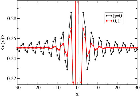
Figure 4: Friedel oscillations of the flux line density vs. distance $x$ from the defect, calculated numerically in the free fermion limit ($g=1$) with $\epsilon_{0}=2$ and $n_{0}=0.25$.

Figure 5: Schematic picture of the “traffic jam” scenario, for vortex lines in the vicinity of a columnar pin as described in the text. Because of their mutual repulsion, flux lines queue up in the vicinity of the pin.

III.0.2 Current and Pinning Number

Conservation of “charge”, i.e., the number of flux lines in a slab, implies the existence of a conserved current operator, even in the presence of a pin and a tilt field. This is given by:

$$\hat{J}(x)=-i{d\hat{\cal H}(x)\over dh}={-i\over 2m}\left[\psi^{\dagger}{d\over dx}\psi-\left({d\over dx}\psi^{\dagger}\right)\psi-2h\psi^{\dagger}\psi\right].$$ (81)

In the absence of a pin there is an imaginary current in the ground state,

$$J=<0|J(x)|0>={ih\over m}<0|\psi^{\dagger}(x)\psi(x)|0>=ihn_{0}/m.$$ (82)

Physically, this current describes vortex lines tilted at an angle of $\tan^{-1}(h/m)$ relative to the $\tau$-axis. Equivalently, each boson has an average imaginary-time “velocity” of $h/m$. Intuitively we might expect that the pin would reduce this current since vortices tend to get “stuck” on it. However, the current is conserved and further describes a $\tau$-independent vortex density, even in the presence of a pin. Thus it has the same value in the vicinity of the pin as everywhere else in the sample. Although a single pin cannot change the value of the current in the limit $L\to\infty$, this defect nevertheless can have important finite size effects on the current which we now consider. We find it convenient to define a “pinning number”, $N_{p}$, which describes the finite size reduction of the current due to the pin. Setting $J\equiv<0|\hat{J}(x)|0>\equiv(ih/mL)(N-N_{p})$, thus defining

$$N_{p}\equiv N[J(0)-J(\epsilon_{0})]/J(0)=N+imLJ(\epsilon_{0})/h.$$ (83)

Since we may think of each boson as contributing $ih/mL$ to the current in the clean system, $N_{p}$ measures the effective number of bosons which are not contributing to the current because they are “stuck” in the vicinity of the pin. We are considering a finite size effect since we expect that $J(\epsilon_{0})-J(0)\propto 1/L$.

$N_{p}$ may be readily calculated in the dilute limit where we can use the free fermion approximation. The simplest procedure is to calculate the ground state energy and then differentiate to get the current using:

$$J={-i\over L}{dE_{0}\over dh},$$ (84)

which follows from Eq. (81). The ground state energy, $E_{0}(h)$ may be calculated by summing up all single particle levels below the “Fermi surface”, as indicated by the prime in the summation:

$$E_{0}=\sum_{n}{{}^{\prime}}{K_{n}^{2}\over 2m},$$ (85)

where the $K_{n}$ are given by Eqs. (71) and (73) for the extended states.

We will assume that the limit $L\to\infty$ is being taken in Eq. (83) so that we only need the energy to O(1/L). In this way we obtain:

$$J(\epsilon_{0})={ihn_{0}\over m}+{i\over 2\pi mL}\left[k_{F}\ln{k_{F}^{2}+h^{2}\over k_{F}^{2}+(h-m\epsilon_{0})^{2}}+ih\ln{(k_{F}+ih)[k_{F}-i(h-m\epsilon_{0})]\over(k_{F}-ih)[k_{F}+i(h-m\epsilon_{0})]}\right].$$ (86)

(Here $k_{F}=\pi n_{0}$.) Upon extracting the pinning number, $N_{p}$, from Eq. (86), we have:

$$N_{p}=-{1\over 2\pi h}\left[k_{F}\ln{k_{F}^{2}+h^{2}\over k_{F}^{2}+(h-m\epsilon_{0})^{2}}+ih\ln{(k_{F}+ih)(k_{F}-i(h-m\epsilon_{0}))\over(k_{F}-ih)(k_{F}+i(h-m\epsilon_{0}))}\right].$$ (87)

Despite the fact that there is a bound state for $h<m\epsilon_{0}$ but not for $h>m\epsilon_{0}$, $N_{p}$ is a smooth function of $h$ near $m\epsilon_{0}$ in this large $L$ limit. (However, a step develops at $h=m\epsilon_{0}$ in the limit $k_{F}\to 0$.) In the limit $h<<\pi n_{0}$, we find the asymptotic behaviors at large and small $\epsilon_{0}$:

$$N_{p} \to {(m\epsilon_{0})^{2}\over 2\pi^{2}n_{0}h},\ \ (m\epsilon_{0}<<h)$$ (88)

$$\to {n_{0}\over h}\ln(|\epsilon_{0}|/n_{0}),\ \ (m\epsilon_{0}>>h,n_{0}).$$

Remarkably, the pinning number diverges as $h\to 0$. This behavior can be understood in terms of the Friedel oscillations discussed in the previous sub-section. These oscillations imply a local density wave which extends out to a distance of $O(1/h)$ away from the pin as illustrated in fig. 5. We may think of the particles as entering a sort of “traffic jam” near the pin similar to the one which may occur near a toll booth. Heuristically, we think of each particle as waiting at the locations of the peaks in the density, which have spacing $1/n_{0}$, until the particle in front has moved ahead one space. The pin at $x=0$ corresponds to the toll booth. Unlike most real traffic jams at toll booths, this one is symmetric under $x\to-x$. The number of particles participating in the traffic jam is $O(1/h)$ and represents the number of particles which are not participating in the current.

It is important to note here that we have taken the limit $L\to\infty$ first before considering small $h$. That is, we are assuming $L>>1/h$. The behavior of the current as $h\to 0$ with fixed $L$ is quite different, becoming linear in $h$. In this linear response regime the non-Hermiticity of the Hamiltonian becomes unimportant since the linear response to the imaginary vector potential can be expressed in terms of the susceptibility calculated at $h=0$. Apart from a factor of $i$, this is the same as the linear response to a real vector potential. A constant real vector potential of strength $-ih$ corresponds to a dimensionless magnetic flux, $ihL$ threading the ring. The resulting real current is known as the persistent current. It has been discussed for the case of a localized impurity potential in a Luttinger liquid, by Gogolin and Prokof’ev.Gogolin In the case of non-interacting fermions, these authors find an expression for the persistent current in terms of the transmission coefficient at the Fermi surface, $T_{F}$. For the particular case of the $\delta$-function potential of Eq. (21), the transmission coefficient is given by:

$$T_{F}={k_{F}^{2}\over k_{F}^{2}+(m\epsilon_{0})^{2}}.$$ (89)

The Gogolin-Prokof’ev formula for the persistent current, in the limit where the flux goes to zero, for the case of $N$ odd [Eq. (1) of Ref. (Gogolin, )] then gives:

$$J\to{ihn_{0}\over m}{\pi n_{0}\over m\epsilon_{0}}\tan^{-1}\left({m\epsilon_{0}\over\pi n_{0}}\right).$$ (90)

Note that this result, linear in $h$, is independent of $L$. Naturally, at $\epsilon_{0}\to 0$, it reduces to our previous result for the system with no impurity. Of course, once we go beyond linear order the dependence of the current on a (real) flux is very different than its dependence on an imaginary vector potential $h$. In particular the flux dependence is periodic with period $2\pi$ and is $O(1/L)$. We expect the imaginary current to cross over from the large $L$ result to the linear response regime when $1/h$ is of order $L$. At this point the “traffic jam” is filling the entire system.

In the limit $\epsilon_{0}\to\infty$, tunnelling of particles past the pin becomes very ineffective. It is then instructive to rederive our results using a weak tunnelling model. This approach will be very useful in Sec. IV when we consider the case $g<1$. In the dilute limit we can again analyse a non-interacting fermion problem. It is convenient to consider a non-interacting fermionic tight-binding model with a weak link between sites $L$ and $1$:

$$H=-t\sum_{i=1}^{L}[e^{-h}c^{\dagger}_{i}c_{i+1}+e^{h}c^{\dagger}_{i+1}c_{i}]-\Gamma[e^{-h}c^{\dagger}_{L}c_{1}+e^{h}c^{\dagger}_{1}c_{L}],$$ (91)

where $\Gamma<<t$ represents the weak link caused by an impurity with very large $\epsilon_{0}$. Here $c_{i}$ is a fermion annihilation operator. For some purposes it is more convenient to make a similarity transformation to a different Hamiltonian which has the same (right and left) eigenvalues, chosen so that all the non-Hermiticity resides on the weak link. This transformation is equivalent to the replacement:

$$c_{j} \to c_{j}e^{hj}$$

$$c_{j}^{\dagger} \to c_{j}^{\dagger}e^{-hj}.$$ (92)

This non-unitary, commutation-relation preserving transformation changes the Hamiltonian to:

$$\tilde{H}=-t\sum_{i=1}^{L}[c^{\dagger}_{i}c_{i+1}+h.c.]-\Gamma[e^{-hL}c^{\dagger}_{L}c_{1}+e^{hL}c^{\dagger}_{1}c_{L}].$$ (93)

The lattice Schroedinger equation associated with $\tilde{H}$ is:

$$-t(\psi_{j-1}+\psi_{j+1}) = E\psi_{j}\ \ (j\neq 1,L)$$

$$-t\psi_{2}-\Gamma e^{-hL}\psi_{L} = E\psi_{1}$$

$$-t\psi_{L-1}-\Gamma e^{hL}\psi_{1} = E\psi_{L}.$$ (94)

To find the scattering states we use the ansatz:

$$\psi_{j}=Ae^{iKj}+Be^{-iKj},$$ (95)

where $A$ and $B$ are amplitudes and $K$ will, in general, be complex. Without loss of generality, we may assume ${\it Im}K\geq 0$. The eigenvalues are then:

$$E(K)=-2t\cos K.$$ (96)

The last two equations of (94) can be rewritten as:

$$\Gamma e^{-hL}\left(Ae^{iKL}+Be^{-iKL}\right) = t(A+B)$$

$$\Gamma e^{hL}\left(Ae^{iK}+Be^{-iK}\right) = t\left[Ae^{iK(L+1)}+Be^{-iK(L+1)}\right]$$ (97)

Upon solving for $A/B$ and simplifying we find an equation which determines the eigenvalues, i.e. the $K$’s:

$$-2\Gamma t\cosh(Lh)\sin K-\Gamma^{2}\sin K(L-1)+t^{2}\sin K(L+1)=0.$$ (98)

For large $Lh$, we see that $K$ must have the form:

$$K_{n}=ih+2\pi n/L+i\phi(K_{n})/L,$$ (99)

as before. [We are interested in the small $\Gamma$ case, where a bound state occurs, so $K_{n}$ is given by the first line in Eq. (71).] After dropping terms suppressed by $e^{-hL}$ (we assume $h>0$), we find:

$$-\Gamma t\sin(ih+k)+{\Gamma^{2}\over 2i}e^{-h+ik+\phi}-{t^{2}\over 2i}e^{h-ik+\phi}=0.$$ (100)

Here we have set $k=2\pi n/N$ and dropped the subscript $n$. We can now determine $\phi$ as a function of $k$.

Once we have $\phi(k)$, we can calculate the ground state energy and hence the current using:

$$E_{0}=-2t\sum_{K}\cos K.$$ (101)

Here we again sum over all energies whose real parts lie below the Fermi surface.

Let us now just focus on the small $\Gamma$ limit. In this limit we may drop the second term from Eq. (100). It is interesting to note that this approximation corresponds to dropping the second term from Eq. (98), which in turn, corresponds to setting $\Gamma e^{-hL}$ to zero in the first of Eq. (97). Thus we consider a “one way” model which ignores the hopping from $1$ to $L$ but allows it from $L$ to $1$. Eq. (100) then reduces to:

$$\Gamma e^{Lh}\sin K=\sin K(L+1).$$ (102)

Note that, in this small $\Gamma$ limit, $\Gamma$ and $h$ only appear in the combination $\Gamma e^{Lh}$. It is therefore convenient to define a shifted $h$ variable:

$$e^{Lh^{\prime}}\equiv\Gamma e^{Lh},$$ (103)

and define $\phi^{\prime}$ by Eq. (99) with $h$ replaced by $h^{\prime}$. Thus:

$$\phi^{\prime}=\phi-\ln\Gamma.$$ (104)

The dominant correction to the current, for small $\Gamma$, is given by using the formula for the current with no pin, and replacing $h$ by $h^{\prime}$. The redefined phase shift is now determined by:

$$e^{\phi^{\prime}}=1-e^{2iK}.$$ (105)

At this point it is convenient to take the continuum limit, assuming that $|h+ik|<<1$, so that the phase shifts become:

$$\phi^{\prime} = \ln(-2iK),$$

$$\phi = \ln(-2iK\Gamma).$$ (106)

Upon comparing to Eq. (73), we see that Eq. (106) is the same formula for the phase shift obtained from the original Hamiltonian in the limit of large $\epsilon_{0}$, with the replacement: $1/m\epsilon_{0}\to 2\Gamma$. The corresponding current is:

$$J={ih^{\prime}n_{0}\over m}+{in_{0}\over mL}\ln(n_{0}m).$$ (107)

Upon using Eq. (103), our final result for the current becomes:

$$J={ihn_{0}\over m}+{in_{0}\over mL}\ln(\Gamma n_{0}m).$$ (108)

Because this analysis applies in the limit $\Gamma\to 0$ we see that Eq. (108) represents a reduction of the current. The leading dependence on $\Gamma$ follows immediately from the formula for the current with no pin upon the replacement of $h$ by $h^{\prime}$ defined by Eq. (103):

$$h\to h^{\prime}=h+{\ln\Gamma\over L}.$$ (109)

The corresponding pinning number is:

$$N_{p}=N+imLJ(\Gamma)/h=-{n_{0}\over h}\ln\Gamma.$$ (110)

This diverges logarithmically, as $\Gamma\to 0$, i.e. as the pinning strength goes to infinity. It agrees with the large $\epsilon_{0}$ result, Eq. (88), with the identification $\Gamma=n_{0}/\epsilon_{0}$.

We have also calculated the pinning number via exact diagonalization of the noninteracting fermion tight–binding model (80). [See Fig. (6).] As expected from (88), $N_{p}$ in fact grows, with decreasing $h$, as $1/h$ until at $h\propto 1/L$ this divergence is cut off due to finite-size effects. As a result, in the linear response limit $Lh\to 0$ the pinning number saturates at a value $N_{p}\propto N$ where $N$ is the total number of bosons. Another prominent feature is a steplike decrease of $N_{p}$ close to $h_{c}=m\epsilon_{0}$, which is a vestige of the single vortex depinning transition.hatano97 After being smeared out by interactions this step is only visible at low filling.

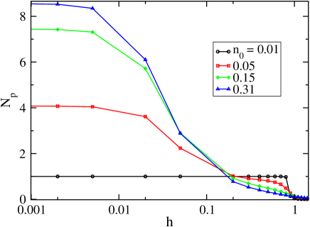
Figure 6: Pinning number in the free fermion limit ($g=1$) for $L=100$ and $\epsilon_{0}=2$. Note the strong enhancement at small tilt $h$ and the “step” at $h_{c}\approx m\epsilon_{0}$ due to single–vortex depinning.

IV Renormalization group approach to general $g$

As noted in Sec. IIC, when $h=0$, a pin is a relevant perturbation for $g<1$ and irrelevant for $g>1$. We use the hydrodynamic approach, involving the dimensionless displacement field, $\theta(x,\tau)$, defined in Sec. IIB. Upon introducing the impurity via Eq. (19), keeping only the most relevant parts of $\hat{n}(0)$, from Eq. (13), and including the tilt field from Eq. (47), the Lagrangian density becomes:

$${\cal L}_{\theta}={\pi\over 2g}\left[{1\over c}\left({\partial\theta\over\partial\tau}\right)^{2}+c\left({\partial\theta\over\partial x}\right)^{2}\right]+h\partial_{\tau}\theta-\left[\epsilon_{0}{d\theta\over dx}+\tilde{\epsilon}_{0}\cos(2\pi\theta)\right]\delta(x),$$ (111)

where $\tilde{\epsilon}_{0}\propto\epsilon_{0}$, the pinning strength, but includes effects of eliminating short distance modes. The lowest order renormalization group scaling equations for these 2 boundary interactions are well known. We study the scaling of the dimensionless quantities $\epsilon_{0}$ and $\tilde{\epsilon}_{0}$, considering the effect of eliminating short distance degrees of freedom of $\theta$, thus reducing the short distance cut-off $\Lambda$. $\epsilon_{0}$ is unchanged by this reduction, indicating that it is a marginal coupling constant. In fact, we may eliminate this term completely by the transformation:

$$\theta(x)\to\theta(x)+{\epsilon_{0}g\over 2\pi c}sgn(x)$$ (112)

where $sgn(x)$ is the sign function with $sgn(0)=0$. This transformation has no effect on the $\cos[2\pi\theta(0))]$ or $\partial\theta/\partial\tau$ terms in Eq. (111). This transformation, Eq. (112), shifts the density of bosons by $(\epsilon_{0}g/\pi c)\delta(x)$. Thus, the $\epsilon_{0}$ term in Eq. (111) is an exactly marginal interaction. On the other hand, the $\tilde{\epsilon}_{0}$ term has a $g$-dependent scaling equation.

IV.1 $h$=0 case

We can determine the scaling equation for $\tilde{\epsilon}_{0}$ by observing that if we integrate out Fourier modes of $\theta$ with wave-vectors between $\Lambda_{0}$ and $\Lambda$ then $\cos u(x,\tau)$ gets replaced by:

$$\cos 2\pi\theta\to\left({\Lambda\over\Lambda_{0}}\right)^{g}\cos 2\pi\theta,$$ (113)

implying that the operator $\cos 2\pi\theta$ has a renormalization group scaling dimension of $g$. Noting that the $\tilde{\epsilon}_{0}$ term in the action involves a $\tau$-integral but no $x$-integral, due to the $\delta(x)$ factor, we see that

$$\tilde{\epsilon}_{0}\to\tilde{\epsilon}_{0}\left({\Lambda\over\Lambda_{0}}\right)^{g-1}.$$ (114)

Equivalently we may write the RG scaling equation:

$${d\over dl}\tilde{\epsilon}_{0}=(1-g)\tilde{\epsilon}_{0},$$ (115)

where $l\equiv\ln(\Lambda_{0}/\Lambda)$. The dimensionless pinning strength gets larger at longer length scales for $g<1$, but gets smaller for $g>1$.

This model, Eq. (111), has been well-studied in the closely related context of a quantum fermion systemKane or a quantum spin chainEggert with a point impurity, from which it arises by bosonization. In these contexts it has been rather well established by numerical and analytic work that, for $g<1$, starting even with a small impurity strength the long distance (low energy) behavior is that of a “cut chain” with the large impurity strength effectively decoupling the two sides. On the other hand, for $g>1$, starting even with a large impurity strength the long distance behavior is that of a “healed” chain with no impurity. We believe that this is also the case for the bosonic version of the model, defined by Eq. (21).

The cut chain fixed point is easily studied in the phase boson representation. A boundary condition, $\theta(0)=0$ must be imposed. Note that we should really think of the $x>0$ and $x<0$ parts of the systems as being independent in this limit. (We take $L\to\infty$ for this discussion.) Thus we get two boundary conditions, $\theta(0^{\pm})=0$. These imply $\partial\theta/\partial t\propto\Pi_{\theta}=0$ and hence, from Eq. (34), the Neumann boundary condition on $\phi$:

$${d\phi\over dx}(0^{\pm})=0.$$ (116)

This boundary condition modifies the correlation functions. Of course any correlation function of two fields on opposite sides of the pin is zero. The correlation function of two fields on the same side is also modified. One way of calculating these correlation functions, with the boundary condition, is to decompose the free boson fields $\phi$ into left and right moving components:

$$\phi(x,t)=\phi_{L}(t+x/c)+\phi_{R}(t-x/c)$$ (117)

(The most general solution of the equations of motion, $(\partial_{t}^{2}-c^{2}\partial_{x}^{2})\phi=0$ can be decomposed in this way.) Eqs. (34) and (42) then imply:

$$\theta(x,t)={g\over\pi}[\phi_{L}(t+x/c)-\phi_{R}(t-x/c)].$$ (118)

The boundary condition can thus be written:

$$\phi_{L}(t,0^{\pm})=\phi_{R}(t,0^{\pm}).$$ (119)

Let us focus on correlations for $x>0$, for example. Then the boundary condition of Eq. (119) implies, since $\phi_{R,L}$ is a function of $t\mp x/c$ only, that we may regard $\phi_{R}(x)$ as the analytic continuation of $\phi_{L}(x)$ to the negative axis:

$$\phi_{R}(x)\equiv\phi_{L}(-x),\ \ (\hbox{for}\ x>0).$$ (120)

This has the effect of making the density and boson creation operators bi-local:

$$\psi^{\dagger}(x) \approx \sqrt{n_{0}}e^{i[\phi_{L}(x)+\phi_{L}(-x)]}$$

$$n(x)-n_{0} \approx {2g\over\pi}{d\phi_{L}\over dx}+\hbox{constant}\times\cos\{2\pi n_{0}x+2g[\phi_{L}(x)-\phi_{L}(-x)]\}.$$ (121)

The correlation functions can now be calculated using:

$$<\phi_{L}(x,\tau)\phi_{L}(y,0)>=-{1\over 4g}\ln[(x-y)+ic\tau]+\hbox{constant}$$ (122)

Thus the correlation function of the boson creation operator, discussed in Sec. IIC, becomes:

$$<\psi^{\dagger}(x,\tau)\psi(y,0)>\propto\left\{xy\over[(x-y)^{2}+c^{2}\tau^{2}][(x+y)^{2}+c^{2}\tau^{2}]\right\}^{1/4g},$$ (123)

where $x$ and $y$ are on the same side of the pin. Note that in the limit $x,y>>|x-y|,c|\tau|$ we recover the bulk behavior [Eq. (55)]:

$$<\psi^{\dagger}(x,\tau)\psi(y,0)>\propto\left\{1\over[(x-y)^{2}+c^{2}\tau^{2}]\right\}^{1/4g}.$$ (124)

On the other hand, in the limit $c|\tau|>>x,y$ we obtain the “boundary critical behavior”:

$$<\psi^{\dagger}(x,\tau)\psi(y,0)>\propto\left\{1\over|\tau|\right\}^{1/g}.$$ (125)

Thus we see that the operator, $\psi^{\dagger}$, which has a bulk scaling dimension of $1/4g$ has a boundary scaling dimension which is twice as big, $1/2g$. To understand this result, note that, without the boundary condition, $\phi_{L}$ and $\phi_{R}$ are independent fields, so that both factors $e^{i\phi_{L}}$ and $e^{i\phi_{R}}$ contribute equal amounts $1/8g$ to the scaling dimension of $\psi^{\dagger}$. After imposing the boundary condition $\psi^{\dagger}(0)$ becomes the operator $e^{2i\phi_{L}(0)}$ which has dimension $1/2g$.

When the pin is relevant, $g<1$, we may calculate the density oscillations at long distances from the pin by assuming that $\tilde{\epsilon}_{0}\to\infty$ and using the Neumann boundary condition of Eq. (116). This constraint leads to Eq. (121) which leads to:

$$<0|n(x)|0>\to n_{0}+{\hbox{constant}\cdot\cos(2\pi n_{0}x)\over|x|^{g}}.$$ (126)

For an irrelevant pin, we expect the result of lowest order perturbation theory in $\epsilon$ to be valid at long distances, giving Eq. (54). Note this involves a different (larger) exponent than the one which occurs for a relevant pin. These density oscillations are the bosonic version of the generalized Freidel oscillations discussed for fermionic systems and spin chains in Ref. (Friedel, ; Meden02, ).

We can now study the stability of the cut chain fixed point. As discussed above, in this limit the system decouples into two separate sections to the left and right of the pin. If $\tilde{\epsilon}_{0}$ is very large but finite, there will be a (dimensionless) weak tunnelling matrix element, $\Gamma\propto 1/\tilde{\epsilon}_{0}$, between the two sides. In the $\psi$ representation, this effective Hamiltonian is:

$$\hat{H}=\hat{H}_{-}+\hat{H}_{+}-\Gamma c[\psi^{\dagger}(0^{-})\psi(0^{+})+h.c.]$$ (127)

Here

$$\hat{H}_{+}=\int_{x>0}dx{1\over 2m}{d\psi^{\dagger}\over dx}{d\psi\over dx}+\hbox{constant}*\psi^{\dagger}(0)\psi(0)+{1\over 2}\int_{x,y>0}dxdy\hat{n}(x)V(|x-y|)\hat{n}(y),$$ (128)

$H_{-}$ is defined similarly. (Alternatively, an interaction term similar to that in Eq. (23) may be maintained between the two sides. The important thing is that there is no motion of bosons across the pin in this limit.) This is conveniently written in terms of the phase boson, $\phi$ with the boundary condition $d\phi/dx=0$ at $x=0^{\pm}$. Thus we get two copies of the Lagrangian of Eq. (40) for $x>0$ and $x<0$. As explained above, the tunnelling term, analogous to a Josephson coupling across the weak link, becomes:

$$-\Gamma c\psi^{\dagger}(0^{-})\psi(0^{+})+h.c.\propto\Gamma\cos 2[\phi_{L}(0^{+})-\phi_{L}(0^{-})],$$ (129)

of scaling dimension $1/g$. (Because $\psi(0^{+})$ and $\psi(0^{-})$ become independent operators upon imposing the boundary condition, their scaling dimensions simply add. ) Thus, the renormalization group equation obeyed by $\Gamma$ is:

$${d\over dl}\Gamma=\left(1-{1\over g}\right)\Gamma+\ldots$$ (130)

We conclude that a weak tunnelling across the pin is relevant for $g>1$ but irrelevant for $g<1$, i.e. precisely the inverse of the situation for a weak pinning potential, $\tilde{\epsilon}_{0}$. This implies consistency of the bold assumptions that a weak $\tilde{\epsilon}_{0}$ will renormalize all the way to the broken chain fixed point (corresponding to $\Gamma\to 0$) for $g<1$ and that even a large $\tilde{\epsilon}_{0}$ will renormalize to $0$ for $g>1$. We present numerical evidence to verify this conjecture in Appendix C and D.

IV.2 Density oscillations for $h>0$

We now consider the effect of a non-zero transverse field, $h$, in Eq. (111). We may eliminate the term in Eq. (111) proportional to $h$ by a shift of the $\theta$ field:

$$\theta(x,\tau)\to\theta(x,\tau)-(gch/\pi)\tau.$$ (131)

Let us first consider the density oscillations in the limit of a weak pin, in lowest order perturbation theory in $\tilde{\epsilon}_{0}$ as in Sec. IIC. The singular part of the density-density correlation function picks up an extra $h$-dependent phase from this shift:

$$<n(x,\tau)n(0)>\to n_{0}^{2}+{gc^{2}\over 2\pi^{2}}{c^{2}\tau^{2}-x^{2}\over(c^{2}\tau^{2}+x^{2})^{2}}+\sum_{p=1}^{\infty}{A_{p}\cos[(2\pi n_{0}x-2ghc\tau)p]\over[x^{2}+c^{2}\tau^{2}]^{gp^{2}}}+\ldots,$$ (132)

Upon Fourier transforming, we see that the singularities of the structure function have moved off the $q_{x}$ axis to $(q_{x},q_{\tau})=(2\pi n_{0},2ghc)p$, as shown in Fig. (7). The linear response to a static pin is proportional to $S(q_{x},0)$, [see Eq. (53)], which is non-singular, as indicated in Fig. (7). Focussing on what was the leading singularity, at $q_{x}=2\pi n_{0}$, we find:

$$<0|\hat{n}(x)|0>\approx n_{0}+\hbox{constant}\cdot\tilde{\epsilon}_{0}\cdot\cos(2\pi n_{0}x)\int d\tau{e^{i2ghc\tau}\over[x^{2}+c^{2}\tau^{2}]^{g}}.$$ (133)

This integral may be expressed in terms of the modified Bessel function of the second kind, $K_{g-1/2}$:

$$\int d\tau{e^{i(2\pi hn_{0}/m)\tau}\over[x^{2}+c^{2}\tau^{2}]^{g}}={2\over c\xi^{2g-1}\Gamma(g)}\left({\xi\over 2|x|}\right)^{g-1/2}K_{g-1/2}(x/\xi),$$ (134)

with characteristic length scale

$$\xi=cm/(2\pi n_{0}h)=1/(2gh)$$ (135)

and where $\Gamma(g)$ is Euler’s $\Gamma$ function. In the limit $|x|<<\xi$, we obtain the zero tilt result, Eq. (54). In the opposite limit, $|x|>>\xi$, we obtain exponentially screened Friedel oscillations:

$$<0|\hat{n}(x)|0>\approx n_{0}+\hbox{constant}\cdot\tilde{\epsilon}_{0}\cdot\cos(2\pi n_{0}x)e^{-|x|/\xi}{1\over\xi^{g-1}|x|^{g}}.$$ (136)

Beyond the new characteristic length scale, $\xi=1/(2gh)$, we expect that the pin loses its effectiveness in ordering the vortices, for any value of $g$. It is natural to assume that this new length scale acts as an infrared cut-off on the renormalization of the pinning strength, $\tilde{\epsilon}(l)$. Thus the long distance physics should be controlled by:

$$\tilde{\epsilon}_{0}(h)\approx\tilde{\epsilon}_{00}(\Lambda_{0}/h)^{1-g}.$$ (137)

Here $\tilde{\epsilon}_{00}$ is the “bare” value of $\tilde{\epsilon}_{0}$, that is, before renormalization. Provided that $\tilde{\epsilon}_{0}(h)<<1$, we expect the perturbative result to be valid at long distances. Thus it would be valid for $g>1$ even if the bare dimensionless pinning potential is not small, for sufficiently small $h$. It would also be valid for $g<1$ provided that the bare dimensionless pinning potential is sufficiently small and $h$ is not too small. As we showed in the previous section, for the case $g=1$, corresponding to free fermions, this exponential decay of the Friedel oscillations at long distances holds for any $\tilde{\epsilon}_{0}$. Even if the above criteria are not satisfied we still expect exponentially decaying density oscillations at long distances for any values of $g$ and $\tilde{\epsilon}_{0}$ provided that $h\neq 0$.

Figure 7: (a) Reciprocal lattice vectors in the $(q_{x},q_{\tau})$–plane for $h\neq 0$. In contrast to Fig. (2), the singularities now occur off the $q_{x}$–axis, where the potential due to the columnar pin is zero. (b) As shown in this profile, the structure function $S(q_{x},0)$ is now finite and nonsingular everywhere along the $q_{x}$–axis.

DMRG results for the Friedel oscillations with $g<1$ are shown in fig. 8. Note that, as in the free Fermion limit $g=1$, a finite tilt $h$ tends to strongly suppress the oscillations. Our data are consistent with a crossover from power–law to exponential decay with increasing $h$, although the system sizes are too small to extract precise exponents.

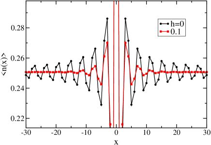
Figure 8: Friedel oscillations calculated by DMRG for $\epsilon_{0}=2$, $U=10$, $V=4$, $L=128$ and $n_{0}=0.25$, corresponding to $g\approx 0.72$.

IV.3 Current

We first consider the case $h\to 0$ for fixed $L$. As discussed in Sec. III, when $hL<<1$, the current becomes linear in $h$ and proportional to the (persistent) current that results from a real vector potential. This real persistent current was analysed, for arbitrary $g$, by Gogolin and Prokof’ev Gogolin and we may simply take over their results, replacing the dimensionless magnetic flux, $\varphi$, by $ihL$. In the case of a relevant pin, $g<1$, Eq. (18) of [Gogolin, ] gives:

$$J\propto{ih\over L^{1/g-1}}.$$ (138)

We see that the linear response current vanishes as a non-trivial power of $1/L$, whereas it is independent of $L$ for $g=1$. As observed in [Gogolin, ] the $L$-dependence of the current can be understood from the renormalization group behavior of the effective weak tunneling matrix element, $\Gamma$, given by Eq. (130),

$$\Gamma(L)\propto L^{1-1/g}.$$ (139)

In the weak tunnelling limit of the non-interacting case ($g=1$), the transmission coeffient $T_{F}\propto|\Gamma|^{2}$ and the persistent current $J\propto\sqrt{T_{F}}\propto\Gamma$. For $g<1$, replacing $\Gamma$ by $\Gamma(L)$, leads to (138). In the other case of an irrelevant pin, $g>1$, the transmission coefficient renormalizes to $1$ at low energies and long distances so we expect to recover the result for the system with no pin, namely

$$J\to{ih\over m}n_{0}.$$ (140)

(Note that we require not only $1/h>>L$ but also that $L$ is much greater than the characteristic length scale required to send $\tilde{\epsilon}_{0}\to 0$. )

In fig. 9 we show DMRG results for the imaginary current in the case of a relevant pin for system sizes up to $L=256$. The finite–size scaling (138) of the linear–response current is confirmed with high accuracy in the limit $hL\leq 1$.

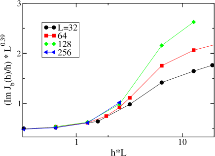
Figure 9: Finite–size scaling of the current (DMRG results) for filling $n_{0}=0.25$, $\epsilon_{0}=2$ and a relevant pin ($g\approx 0.72$). Note the data collapse in the linear–response regime $hL\to 0$.

We now consider the other limit, $L>>\xi\equiv 1/2gh$, where we can characterize the current in terms of the pinning number, $N_{p}$. In the case, $g>1$, where the pin is irrelevant, it is reasonable to calculate the correction to the current due to the pin (which can be expressed in terms of the pinning number) in lowest order perturbation theory in $\tilde{\epsilon}_{0}$, using the bosonized $\theta$-representation. We again start with the Lagrangian density of Eq. (111).

In second order perturbation theory in $\tilde{\epsilon}_{0}$, the leading correction to the ground state energy is proportional to:

$$\delta E_{0}\propto\tilde{\epsilon}_{0}^{2}\int_{-\infty}^{\infty}d\tau<\cos[2\pi\theta(0,\tau)]\cos[2\pi\theta(0,0)]>.$$ (141)

Note that this ground state energy is given by the logarithm of the classical partition function associated with Eq. (111). Upon taking into account the shift of Eq. (131), we find:

$$\delta E_{0}\propto\tilde{\epsilon}_{0}^{2}\int_{\tau_{0}}^{\infty}{d\tau\over|\tau|^{2g}}\cos[2gch\tau],$$ (142)

where $\tau_{0}$ is a short distance cut-off. For $2<2g<3$, Eq. (142) leads to:

$$\delta E_{0}\propto\tilde{\epsilon}_{0}^{2}\left[-h^{2g-1}+\hbox{constant}\cdot\tau_{0}^{-2g+1}\right].$$ (143)

The correction to the current due to the pin, is thus:

$$\delta J = {-i\over L}{d\delta E_{0}\over dh}\propto{i\over L}\tilde{\epsilon}_{0}^{2}h^{2g-2}$$ (144)

$$\propto {i\over L}\tilde{\epsilon}_{0}(h)^{2}.$$

The last entry expresses $\delta J$ in terms of the renormalized pinning strength at the length scale $1/h$. After setting $g=1$, we find agreement with the exact result in the dilute limit, if we also assume that $h<<\pi n_{0}$. We only expect the phonon representation to be valid when $h<<\pi n_{0}$ since $n_{0}$ represents an effective ultra-violet cut off and we have thrown away higher derivative terms in deriving this effective Lagrangian. For $2g>3$, the leading behavior at small $h$, from Eq. (142), is:

$$\delta J\propto{i\over L}\tilde{\epsilon}_{0}^{2}h/\tau_{0}^{2g-3}.$$ (145)

Thus the pinning number behaves as:

$$N_{p} \propto {\tilde{\epsilon}_{0}^{2}\over h^{3-2g}}\ \ (2<2g<3)$$ (146)

$$\propto \tilde{\epsilon}_{0}^{2}\ \ (2g>3),$$

results applicable in the limit $Lh\to\infty$.

We may straightforwardly extend this calculation to finite $Lh$. Then we must use the finite $L$ version of the correlation function in Eq. (141), which can be obtained by a conformal transformation and effectively replaces $\tau$ by $(L/\pi c)\sinh(\pi c\tau/L)$ in Eq. (142). Upon rescaling the $\tau$ integration variable, $u\equiv\pi c\tau/L$, and using Eq. (36), we obtain:

$$\delta E_{0}\propto\tilde{\epsilon}_{0}^{2}(L/\pi c)\int_{1/(\pi c\tau_{0}/L)}^{\infty}{du\over|(L/\pi)\sinh u|^{2g}}\cos[2ghLu/\pi],$$ (147)

Differentiating with respect to $h$ and dividing by $h$ gives the pinning number:

$$N_{P}\propto\tilde{\epsilon}_{0}^{2}L^{2-2g}h^{-1}\int_{0}^{\infty}du{u\sin(2ghLu/\pi)\over\sinh^{2g}u},\ \ (1<g<3/2).$$ (148)

Note that we have set the lower limit of the integral to $0$ since it converges. Thus we obtain the scaling form:

$$N_{p}=L^{3-2g}f(Lh),$$ (149)

where:

$$f(x)\propto{1\over x}\int_{0}^{\infty}du{u\sin(2gux/\pi)\over(\sinh u)^{2g}}.$$ (150)

We see that $f(x)\to x^{2g-3}$ as $x\to 0$. Using DMRG, we have numerically checked this scaling for the case $2g<3$ and have found good agreement (see fig. 10).

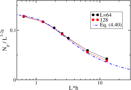
Figure 10: Scaling function for the pinning number in the case of an irrelevant pin ($U=10$, $V=0$, $g\approx 1.19$) with boson density $n_{0}=0.25$ and pinning potential $\epsilon_{0}=2$.

To study the case of a relevant pin, $g<1$, we use the weak tunnelling model of Eq. (127). We determined the effective $\Gamma$ parameter by using the $h=0$ RG equations of Eq. (130) out to a length scale of $1/h$:

$$\Gamma\propto h^{1/g-1}.$$ (151)

We noted in Sec. III that it is convenient to make a similarity transformation of the Hamiltonian such that the hopping terms have the form of Eq. (93) in which all the non-Hermiticity resides on the weak link. We then showed that the exponentially small hopping term, $\propto\Gamma e^{-hL}$ from right to left can be dropped at small $\Gamma$, keeping only the exponentially large hopping term, $\propto\Gamma e^{hL}$ from left to right. Thus we have a “one-way hopping model”. It seems plausible that this approximation can also be made away from the $g=1$ free fermion case, as long as the effective $\Gamma$ is very small. Once we make this approximation, $\Gamma$ and $h$ appear only in the combination $\Gamma e^{hL}$. Then, since we expect that, in the infinite $L$ limit the current goes as: $i{n_{0}\over m}h$, the finite size correction at small $\Gamma$ must go as:

$$J\approx i{n_{0}\over m}\left[h+{\ln\Gamma\over L}\right].$$ (152)

We now replace $\Gamma$ by its value in Eq. (151) which leads to:

$$J\approx i{n_{0}\over m}\left[h+{1\over L}\left\{\left({1\over g}-1\right)\ln h+\hbox{constant}\right\}\right].$$ (153)

Thus the pinning number is:

$$N_{p}=N_{b}{J(\tilde{\epsilon}_{0}=0)-J(\tilde{\epsilon}_{0})\over J(\tilde{\epsilon}_{0}=0)}={n_{0}\over h}\left[\left({1\over g}-1\right)|\ln h|+C\right],$$ (154)

where $C$ is a non-universal constant. Note that the universal number $g$ appears here as an amplitude, not as an exponent. We emphasize that we expect this amplitude to be universal by this argument, although the sub-dominant constant is not. Thus a relevant pin only increases the pinning number by a factor of $|\ln h|$ compared to the free fermion (low vortex density) case where the pin is marginal.

Our DMRG results for $N_{p}$ in the $g<1$ case, shown in fig. 11, confirm these analytic predictions. The logarithmic behavior (154) is clearly observed for two different values of the Luttinger liquid parameter $g$. Note that at $Lh\propto 1$ the divergence of $N_{p}$ is cut off, analogous to the free–fermion limit.

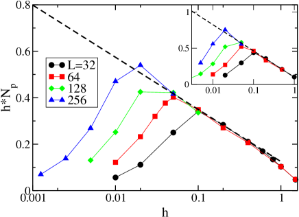
Figure 11: DMRG results for the pinning number. Main plot: filling $n_{0}=0.25$, $\epsilon_{0}=2$ and a relevant pin ($U=10$, $V=4$, corresponding to $g\approx 0.72$). The dashed line gives the logarithmic behavior in Eq. (154) with $C=0.5$. Inset: same for $U=20$, $V=10$, $g\approx 0.62$ and offset $C=0.4$.

In Appendix F we briefly discuss the phase-boson representation of the weak tunnelling model after the similarity transformation, Eq. (93), for general $g$, pointing out its connection with a model of current interest in string theory.

V Point Disorder

This paper focuses on the physics of thermal fluctuations in very clean (1+1)–dimensional superconducting slabs. The appropriate physical conditions necessary to neglect weak point disorder due to oxygen vacancies, proton irradiation, etc.blatter94 in high $T_{c}$ superconductors are discussed in Appendix E. We can, however, get some insight into the influence of a single extended defect in the presence of strong point disorder using the linear response formalism discussed earlier. A treatment of a single columnar pin in the presence of strong point disorder, including a full renormalization group analysis, will appear in a future publication.polkovnikov

The effect of a quenched random distribution of point pins on vortex arrays in thin superconducting slabs has been discussed in a number of publicationsfisher89a ; hwa93 ; hwa94 . In the presence of point disorder, the background elastic free energy (15) on which we impose a single columnar pin becomes

$$\int dxd\tau\big{\{}\frac{1}{2}c_{11}(\partial_{x}u)^{2}+\frac{1}{2}c_{44}(\partial_{\tau}u)^{2}-\mu_{x}(\partial_{x}u)-\mu_{\tau}(\partial_{\tau}u)$$

$$-h(\partial_{\tau}u)+V_{0}(x,\tau)\,\cos\left[2\pi u(x,\tau)/a_{0}-\beta(x,\tau)\right]\big{\}}.$$ (155)

As pointed out in Ref. fisher89a, , the statistical mechanics associated with Eq. (155) is similar to that of an anisotropic two dimensional random field XY model with, however, no topological defects such as the dislocations shown in Fig. (3). As in charge density wave physicslee , the cosine term acts to locally fix the phase of the (1+1)–dimensional vortex crystal at $\beta(x,\tau)$ with a strength determined by the amplitude $V_{0}(x,\tau)$. The couplings $\mu_{x}(x,\tau)$ and $\mu_{\tau}(x,\tau)$ are zero mean random variables which describe local variations in the preferred density and tilt of the vortex lines induced by the particular configuration of point disorder. At long wavelengths, $\mu_{x}(x,\tau)$ and $\mu_{\tau}(x,\tau)$ renormalize in the same way and can be taken to be Gaussian random variables described by a single variance $\sigma$fisher89a ; hwa94 ,

$$\overline{\mu_{i}(x,\tau)\mu_{j}(x^{\prime},\tau^{\prime})}=\sigma\,\delta_{ij}\,\delta(x-x^{\prime})\,\delta(\tau-\tau^{\prime}),$$ (156)

where $i,j=x,\tau$ and the overbar represents a quenched average over the disorder. We also take $V_{0}(x,\tau)$ to be given by a Gaussian distribution, with variance

$$\overline{V_{0}(x,\tau)V_{0}(x^{\prime},\tau^{\prime})}=\Delta_{0}\,\delta(x-x^{\prime})\,\delta(\tau-\tau^{\prime})$$ (157)

while $\beta(x,\tau)$ is uniformly distributed on the interval $[0,2\pi]$.

When averaged over point pinning, the linear response equation (51) becomes

$$\overline{\delta n(x,\tau)}=-\int dx^{\prime}d\tau^{\prime}\frac{V_{D}(x^{\prime})}{T}\,\overline{C(x-x^{\prime},\tau-\tau^{\prime})},$$ (158)

with

$$C(x-x^{\prime},\tau-\tau^{\prime})=\overline{<n(x,\tau)n(x^{\prime},\tau^{\prime})>_{0}}-\overline{<n(x,\tau)>_{0}}\,\overline{<n(x^{\prime},\tau^{\prime})>_{0}}.$$ (159)

The Fourier space version of these relations reads

$$\overline{\delta n(q_{x},q_{\tau})}=\overline{S(q_{x},q_{\tau})}\,\frac{L_{\tau}\delta_{q_{\tau},0}}{T}\,\hat{V}_{D}(q_{x}),$$ (160)

where

$$\overline{S(q_{x},q_{\tau})}=\overline{<|n(q_{x},q_{\tau})|^{2}>},$$ (161)

and all averages are evaluated in the absence of the columnar defect.

We first set $h=0$ and apply the renormalization group analysis of the bulk statistical physics problem defined above to evaluate $\overline{S(q_{x},q_{\tau})}$ and hence determine the change in vortex density due to a single columnar pin. The recursion relations for the scale-dependent couplings $g(l)$, $\sigma(l)$ and $\Delta_{0}(l)$ arehwa93 ; hwa94 ; cardy ; toner

$$\frac{dg(l)}{dl}=0,$$ (162)

$$\frac{d\sigma(l)}{dl}=C_{1}\Delta_{0}^{2}(l)$$ (163)

$$\frac{d\Delta_{0}(l)}{dl}=2[1-g(l)]\Delta_{0}(l)-C_{2}\Delta_{0}^{2}(l)$$ (164)

where $C_{1}$ and $C_{2}$ are positive constants. The renormalization group flows in the $(g,\Delta_{0})$–plane are shown in Fig. 12.

Figure 12: Renormalization group flows in $g$ and $\Delta_{0}$ for the random field XY model which describes (1+1)–dimensional vortex arrays subjected to point disorder.cardy The Luttinger liquid fixed line at $\Delta_{0}=0$ is is stable to point disorder for $g>1$, which is also the regime where a single columnar pin is irrelevant. This line becomes unstable to a new fixed line where point disorder is important for $g<1$.

The line of fixed points at $\Delta_{0}=0$ in Fig. 12 is stable to point disorder when $g>1$. This is also the regime where columnar pins are irrelevant in pure systems. However, as the point disorder strength tends to zero, it generates via Eq. (163) a nonzero variance for the couplings $\mu_{x}(x,\tau)$ and $\mu_{\tau}(x,\tau)$ in Eq. (155). After setting the cosine coupling to zero in Eq. (155) it is straightforward to showrubinstein that the leading singular term ($m=1$) in Eq. (49) is replaced by

$$\overline{<n(x,\tau)n_{(}0,0)>}-n_{0}^{2}\sim{\cos(2\pi n_{0}x)\over[x^{2}+c^{2}\tau^{2}]^{\eta/2}},$$ (165)

with

$$\eta=2g+\frac{\sigma_{\infty}}{2\pi},$$ (166)

where $\sigma_{\infty}=\lim_{l\to\infty}\sigma(l)$ is a (positive) correction to the Luttinger liquid result. Hence, $\eta>2$ for all $g\geq 1$ and we conclude that $\overline{S(q_{x},q_{\tau})}$ never diverges near any of the reciprocal lattice vectors. In particular, $\overline{S(q_{x},q_{\tau})}$ never diverges at $G_{1}$, suggesting that an isolated columnar pin becomes even more irrelevant for in the presence of strong point disorder when $g>1$.

A new stable line of fixed points appears in Fig. 12 for $g\leq 1$, signaling the onset of a “vortex glass” phase in (1+1)–dimensionsfisher89a . The analysis of Hwa and Fisherhwa94 (see also, Ref. toner, ) shows that

$$\overline{\langle n_{1}(x,\tau)n_{1}^{*}(0,0)\rangle}\sim\exp\left[-C_{3}\ln^{2}(x^{2}+c^{2}\tau^{2})\right]$$ (167)

where $C_{3}$ is a positive constant. Because this decay is faster than any power law, $\overline{S(q_{x},q_{\tau})}$ is again finite everywhere along the $q_{x}$–axis, suggesting that an isolated columnar defect is also asymptotically irrelevant in the presence of strong point disorder in this regime. However, if the point disorder is weak, the effective pinning strength of the columnar defect can grow quite large over intermediate length scales. The subtle and complex physics which distinguishes the response of (1+1)–dimensional vortex arrays to a columnar defect above and below the vortex glass transition will be discussed in Ref. (polkovnikov, ).

We conclude this brief discussion of point disorder with two comments: The tilt field $h$ is a strongly relevant variable in (1+1)–dimensions (the recursion relation for $h$ readshwa93 $dh(l)/dl=h(l)$) for both pure and disordered systems. When point disorder is present, the structure function $\overline{S(q_{x},q_{\tau})}$ can only become less singular along the $q_{x}$–axis as a result of the affine transfomation discussed above for pure systems. Second, the slowly decaying translational correlations which produce interesting physics for vortex arrays in (1+1)–dimensions also appear in the “Bragg glass” phase which arises when the Abrikosov flux lattice is subjected to weak point disorder in (2+1) dimensionsgiamarchi94 . A study of related non-Hermitian Luttinger-liquid-like phenomena when a single twin plane or grain boundary is inserted into bulk vortex arrays with a tilted field and subject to point disorder is currently in progress.polkovnikov

VI Conclusions

We have studied interacting vortices in a thin platelet, in the presence of a single columnar pin, using a combination of exact methods for the dilute limit based on the free fermion representation, field theory methods and numerical techniques. The response to a pin is controlled by the Luttinger liquid parameter, $g$, which depends in a complicated way on the details of the inter-vortex interactions and on the density. When the pin is parallel to the magnetic field, it is an irrelevant perturbation for $g>1$ but a relevant perturbation for $g<1$. In both cases a single pin produces a local vortex lattice with density oscillations that decay as a power law. A transverse magnetic field introduces a new length scale, $1/h$. The density oscillations decay exponentially beyond this distance from the pin. We characterize the imaginary current, or transverse Meissner effect, by a “pinning number”, $N_{p}$, which measures how many vortices are stuck in the vicinity of the pin. This number diverges as $(1/h)|\ln h|$ for $g<1$ but as $h^{2g-3}$ for $g>1$. When $g=1$, the free fermion mapping shows that $N_{p}\propto 1/h$. Even for zero tilt, point disorder drastically modified the critical behavior associated with $g$ passing through $1$. However, it may be possible to experimentally probe non-Hermitian Luttinger liquid physics using sufficiently clean high-$T_{c}$ thin platelets with notches cut on the surface.

Appendix A Critical exponents of the dilute Bose gas

It is well-known that the low energy long distance properties of a Bose gas in the dilute limit (average inter-particle separation, $1/n_{0}$, large compared to interaction range) are given by a gas of free fermions. In the continuum elastic theory, defined in Sec. II, this corresponds to the value $g=1$ of the dimensionless Luttinger liquid parameter which determines all critical properties. In this appendix we derive a general result for the leading correction to this limiting value of $g$, expressing our result in terms of the scattering length, $a$, determined by the boson interaction, $V(x)$ in Eq. (21) and the density, $n_{0}$. Apart from its applications to flux lines in thin platelets, we expect that this formula will be of quite general applicability to various one-dimensional quantum models.

Our result depends critically on two well-known features of the Bose gas. One of them is Eq. (36), $cg/\pi=n_{0}m$. This is expected to be exact for a Galilean invariant gas.Haldane This follows by considering the energy of the entire system lowest energy of momentum $P$. The conserved momentum density is:

$$P(x)={-i\over 2}\left[\psi^{\dagger}{d\over dx}\psi-\left({d\over dx}\psi^{\dagger}\right)\psi\right]\approx n_{0}{d\phi\over dx}.$$ (168)

Thus the lowest energy state with a very low momentum momentum $P$ is one in which $\phi(x)=(Px/n_{0}L)$. From the Hamiltonian in $\phi$-representation, Eq. (35), we see that the energy of this state is:

$$E_{0}(P)={cgP^{2}\over 2\pi n_{0}^{2}L}.$$ (169)

On the other hand, from Galilean invariance the exact energy of this state, which is simply one in which all $N$ bosons are given a boost to a momentum $P/N$ is:

$$E_{0}(P)={P^{2}\over 2mN}.$$ (170)

Comparing these two formulas gives Eq. (36). We note that this argument doesn’t really require exact Galilean invariance; it is enough that the disperson relation be approximately quadratic at small momentum. For instance, a quartic term in the dispersion relation would lead to a $(d\phi/dx)^{4}$ term in the Hamiltonian in $\phi$-representation but wouldn’t interfere with this determination of the coefficient of the $(d\phi/dx)^{2}$ term. We also require an expression for the compressibility in terms of $g$ and $c$. To this end, consider the change in energy of the ground state when a relatively small change, $\delta N$ is made in the number of particles. From Eq. (27), which expresses a uniform density perturbation as $\delta n=d\theta/dx$ and Eq. (41) giving the Hamiltonian in $\theta$-representation, we see that

$$\delta E={c\pi\over 2g}{(\delta N)^{2}\over L}.$$ (171)

Therefore the compressibility, $\kappa$ is given by:

$${1\over\kappa}\equiv{N^{2}\over L}\left({\partial^{2}E_{0}\over\partial N^{2}}\right)_{N}={c\pi\over g}n_{0}^{2}.$$ (172)

Upon combining Eq. (172) with Eq. (36), we see that $g$ is completely determined by $n_{0}$, $m$ and $\kappa$:

$$g=\sqrt{\pi^{2}n_{0}^{3}\kappa\over m}.$$ (173)

We therefore focus on calculating the compressibility $\kappa$ of a dilute Bose gas.

Some general results on dilute Bose gases in (1+1) dimensions were derived in Ref. (Lou, ). There it was argued that, in lowest order approximation, the ground state wave-function can be taken to be of the form which is exact for a continuum $\delta$-function interaction.Lieb If we label the co-ordinates of the $N$ bosons $x_{i}$ and assume $x_{1}<x_{2}<\ldots<x_{N}$, this result takes the form:

$$\Psi(x_{1},x_{2},\ldots x_{N})\approx\sum_{P}A(P)P\exp\left(i\sum_{j=1}^{N}k_{j}x_{j}\right),$$ (174)

for some set of wave-vectors $k_{j}$ ( which must all be different). Here $P$ permutes the $k_{j}$’s and the sum is over all permutations. The $A(P)$ are coefficients to be determined. The many body wave-function,$\Psi$, is determined for other orderings of the $x_{j}$ from the required symmetry of the wave-function which follows from Bose statistics. By considering what happens when two particles approach each other, we can see that:

$$A(Q)=-A(P)e^{i2\delta[(k_{i}-k_{j})/2]}.$$ (175)

Here the two permutations $P$ and $Q$ differ only by interchanging particles $i$ and $j$ and $\delta(k)$ is the even channel phase shift. The quantity $\delta(k)$ is defined by the behavior of the 2-particle wave-function at long distances:

$$\Psi(x_{1}-x_{2})\to\sin[k|x_{1}-x_{2}|+\delta(k)].$$ (176)

At small $k$, the limit which concerns us for low density, the phase shift behaves as:

$$\delta(k)\to-ak,$$ (177)

which we take as the definition of $a$, the scattering length. The periodic boundary conditions give a set of constraints which determine the allowed $k_{i}$’s in terms of the phase shift. In the low density limit these conditions become simply:

$$k_{j}(L-Na)+a\sum_{s}k_{s}=\pi n_{j},\ \ \hbox{all}\ j,$$ (178)

where the integers $n_{j}$ must be all even for $N$ odd and all odd for $N$ even. The solution of these equations can be further simplified in the low density limit, $N/L<<a$. In lowest order we obtain simply:

$$k_{j0}=\pi n_{j}/L,$$ (179)

where the $n_{j}$ are even for $N$ odd but are odd for $N$ even. We may calculate the energy by simply summing the kinetic energy in a region of parameter space where the particles are all far apart:

$$E={1\over 2m}\sum_{j}k_{j}^{2},$$ (180)

so we see that we must choose the smallest possible $k_{j0}$’s to get the ground state corresponding to a “Fermi surface” for 1D bosons. The Fermi wave-vector is determined in the usual way:

$$n_{0}=\int_{-k_{F}}^{k_{F}}{dk\over 2\pi}={k_{F}\over\pi}.$$ (181)

By expanding Eq. (178) to next order we obtain $k_{j}=k_{j0}+\delta k_{j}$, with

$$\delta k_{j}={Na\over L}k_{j0}-{a\over L}\sum_{s}k_{s0}.$$ (182)

Thus, in the limit $L\to\infty$, the ground state energy density to next order is:

$$E_{0}/L\approx{1\over 2m}\int_{-k_{F}}^{k_{F}}{dk\over 2\pi}k^{2}+{a\over 2m}\int_{-k_{F}}^{k_{F}}{dk\over 2\pi}\int_{-k_{F}}^{k_{F}}{dk^{\prime}\over 2\pi}(k-k^{\prime})^{2}.$$ (183)

Upon expressing $k_{F}$ in terms of $n_{0}$ we obtain:

$$E_{0}/L\approx{\pi^{2}n_{0}^{3}\over 6m}+{a\pi^{2}n_{0}^{4}\over 3m}.$$ (184)

We can now obtain a formula for the compressibility, $\kappa$, namely

$${1\over\kappa}\equiv{N^{2}\over L}\left({d^{2}E_{0}\over dN^{2}}\right)_{L}=\pi^{2}\left({n_{0}^{3}\over m}+{4an_{0}^{4}\over m}\right).$$ (185)

From $\kappa$ and Eq. (173) we determine the Luttinger liquid parameter $g$ at low density:

$$g\approx 1-2an_{0}+O(a^{2}n_{0}^{2}).$$ (186)

We note that a quartic correction to the dispersion relation would only correct Eq. (184) and hence $1/\kappa$ at $O(n_{0}^{5})$ and hence lead to a correction to $g$ of $O(n_{0}^{2})$. Therefore, we expect Eq. (186) to be correct even for non-Galilean invariant systems. Applications of this result to spin chains will be discussed elsewhere.Affleck2

Appendix B determining $g$ for the tight-binding models

Our predictions about the critical behavior of the system all involve the parameter $g$. To test these predictions via DMRG on the lattice tight-binding model we need to know $g$ as a function of the microscopic parameters of that model. At low densities we may obtain an analytic formula for $g$ using the general result Eq. (1) together with an exact formula for the scattering length of our tight binding model. For larger densities we must rely exclusively on numerical calculations of quantities, in the tight binding model with no defect and $h=0$, for determination of $g$.

We now calculate the scattering length for the tight-binding model of Eq. (23). To find the phase shift we consider the sector of the Hilbert space with 2 bosons, total momentum zero and even parity (as required by Bose statistics). We may write the eigenstates in terms of the amplitude $\Psi_{j}$ for the 2 bosons to be separated by a displacement $j$. We may also write a lattice Schroedinger equation in this subspace. For $|j|\geq 2$ this equation reads:

$$-2t[\Psi_{j+1}+\Psi_{j-1}]=E\Psi_{j}.$$ (187)

The factor of 2 arises because we can increase the separation of the bosons by hopping either one of them; each process contributes a term $t$. The equations are different for $|j|=1$ or $0$ and read

$$-2t[\Psi_{2}+\Psi_{0}]+V\Psi_{1} = E\Psi_{1}$$

$$-2t[\Psi_{-2}+\Psi_{0}]+V\Psi_{-1} = E\Psi_{-1}$$

$$-2t[\Psi_{1}+\Psi_{-1}]+U\Psi_{0} = E\Psi_{0}.$$ (188)

We write the wave-function as

$$\Psi_{j}=\sin[k|j|+\delta],\ \ (|j|\geq 1),$$ (189)

in agreement with the definition of the phase shift in Eq. (176). Due to the short-range interaction, this ansatz exactly satisfies the Schroedinger equation, with the correct choice of $\Psi_{0}$ and with $E=-4t\cos k$. Upon substituting in Eq. (188), we obtain:

$$-2t[\sin(2k+\delta)+\Psi_{0}]+V\sin(k+\delta) = -4t\cos k\sin(k+\delta)$$

$$-4t\sin(k+\delta)+(U+4t\cos k)\Psi_{0} = 0.$$ (190)

A little algebra gives:

$$\tan\delta={-8t^{2}\sin k+(U+4t\cos k)[(V+4t\cos k)\sin k-2t\sin 2k]\over 8t^{2}\cos k+(U+4t\cos k)[-(V+4t\cos k)\cos k+2t\cos 2k]}.$$ (191)

Upon taking the limit $k\to 0$ we obtain $\delta\to-ak$ with:

$$a=-{8t^{2}-4tV-UV\over 2tU+UV+4tV}.$$ (192)

Note that $a$ diverges as $U$, $V\to 0$ at fixed $t$ as for the continuum $\delta$-function potential. Thus, at low density, the Luttinger liquid parameter, $g$, behaves as:

$$g\to 1+2n_{0}{8t^{2}-4tV-UV\over 2tU+UV+4tV}.$$ (193)

We emphasize that this result is expected to be valid for arbitrarily large positive $U$ and $V$ at low enough $n_{0}$.

We now turn to estimating $g$ from numerical results on finite systems. The most straightforward way of doing this is from the correlation function of $n$ or $\psi$ using Eq. (49) or (55) respectively. Since our numerical results are for finite systems with periodic boundary conditions, we instead use the finite size versions of these formulas which can be obtained by a conformal transformation:

$$<n(x)n(0)> \to n_{0}^{2}+\hbox{constant}\times{\cos(2\pi n_{0}x)\over|L\sin(\pi x/L)|^{2g}}+\ldots$$ (194)

$$<\psi^{\dagger}(x)\psi(0)> \to {\hbox{constant}\over|L\sin(\pi x/L)|^{1/2g}}+\ldots$$ (195)

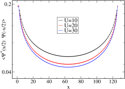
Figure 13: Bosonic correlation function for the lattice model (23) with $L=128$, $V=0$, $n_{0}=0.25$ and $h=0$. Symbols represent DMRG results for the bosonic correlation function and lines are fits based on the conformal field theory prediction (195) with $g=1.19/1.09/1.06$.

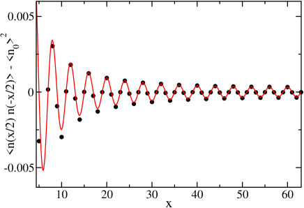
Figure 14: DMRG result for the density correlation function with $U=10$, $V=4$, $L=128$, $n_{0}=0.25$ and $h=0$ (black circles). The red line is a fit based on the CFT formula (194) with $g=0.72$. Note the strong Friedel oscillations due to $g<1$.

Alternatively, g may be extracted from the finite size spectrum in various ways. The compressibility is easily obtained from the energy to add or remove one particle:

$${1\over\kappa}={c\pi\over g}n_{0}^{2}={N^{2}\over L}\left({\partial^{2}E_{0}\over\partial N^{2}}\right)_{L}\approx{N^{2}\over L}[E_{0}(N+1)+E_{0}(N-1)-2E_{0}(N)].$$ (196)

However, we need another result to determine separately the phonon velocity $c$ and the Luttinger liquid parameter $g$. A simple possibility is to measure the speed of sound from the excitation energy of the lowest excited state with wave-vector $k$, choosing the smallest possible non-zero wave-vector, $k=2\pi/L$.

$$E(N,k)-E_{0}(N)\approx c|k|.$$ (197)

Another possibility is to measure the $1/L$ correction to the ground state energy:

$$E_{0}\approx e_{0}L-{\pi c\over 6L},$$ (198)

for a non-universal constant, $e_{0}$. This follows from Refs. (c, ) using the fact that periodic boundary conditions on $\psi$ correspond to periodic boundary conditions on $\phi$ (mod $2\pi$) or $\theta$ (mod 1).

Within our DMRG simulations we have estimated $g$ using the boson correlation function in eq. (195), see Fig. (13). We also show the fit for the density correlations in Fig. (14). The agreement is very good except at short distances where the field theory predictions are expected to fail. We have checked that the values of $g$ so obtained are in very good agreement with the values obtained from the compressibility (196) and the $1/L$ correction to the ground state energy (198). Note that $g$ for the Bose–Hubbard model has been calculated previously by Kühner et al. Kuehner where the authors used periodic boundary conditions in the DMRG algorithm. Our results for $g$ are shown in fig. (15). For small densities the agreement between the asymptotic expression (193) and the numerical data is obviously very good. We expect that with increasing density, $g$ behaves in a non-monotonic fashion and finally approaches $g=1$ again as the filling becomes commensurate in the limit $n_{0}\to 1$. For finite next–neighbor repulsion $V>0$ and $n=0.5$ a charge–density wave instability occursKuehner which we have not studied here. For the main motivation of our work – interacting vortex physics – the Bose–Hubbard model is only applicable in the limit of small filling, since the lattice constant has no direct physical meaning. Most of the results in our paper have been obtained for $n_{0}=0.25$.

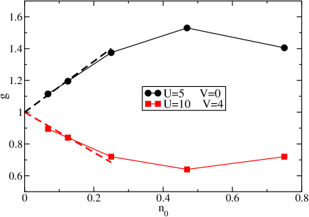
Figure 15: Luttinger–liquid parameter $g$ calculate for the lattice model (23) with $h=\epsilon_{0}=0$ as a function of the boson density $n_{0}$. We have plotted results for two different values of the interaction parameters corresponding to $g>1$ and $g<1$, respectively. The dashed lines show the analytic result (193) at low densities.

Appendix C boson correlation function with a pin

In this appendix we discuss numerical and analytic results on the correlation function of the boson creation operator across a pin, in the absence of a tilt field, $h=0$. This correlation function clearly distinguishes the cases of a relevant ($g<1$) and irrelevant ($g>1$) pin.

We note that the finite $L$ equal time boson correlation function at the broken chain ($\Gamma\to 0$) fixed point, for $x,y>0$, is given by a conformal transformation of Eq. (123):

$$<\psi^{\dagger}(x)\psi(y)>\propto\left\{\sin(\pi x/L)\sin(\pi y/L)\over L^{2}\sin^{2}[\pi(x-y)/2L]\sin^{2}[\pi(x+y)/2L]\right\}^{1/4g}.$$ (199)

This correlation function is now small but non-zero for two points near but on opposite sides of the pin, $x<<L$ and $L-x<<L$. These points are correlated by going around the chain, rather than across the pin. Even for finite $\tilde{\epsilon}_{0}$ we expect this result to hold in the case of a relevant pin, $g<1$, at sufficiently large $L$, $x$, $y$, $N-x$ and $L-y$. We note that neither $x$ nor $y$ can be too close to the pin.

We now consider specifically the boson correlation function across the pin, $<\psi^{\dagger}(x)\psi(-x)>$, ($x>0$) in the limit of infinite system size. If the pin is irrelevant, $g>1$, then at large $x$ we should recover the result for the system with no pin:

$$<\psi^{\dagger}(x)\psi(-x)>\to{\hbox{constant}\over x^{1/2g}}.$$ (200)

On the other hand, if the pin is relevant, $g<1$, this correlation function vanishes more rapidly with $x$. The weak tunnelling, $\Gamma$, model is again useful for this calculation. We may calculate this correlation function in lowest (first) order perturbation theory in $\Gamma$ and then “renormalization group improve” the calculation by replacing $\Gamma$ by its renormalized value at scale $x$. Perturbation theory gives:

$$<\psi^{\dagger}(x)\psi(-x)>\to-\Gamma\int d\tau<\psi^{\dagger}(x,0)\psi(0^{+},\tau)>_{0}<\psi^{\dagger}(0^{-},\tau)\psi(-x,0)>_{0}+c.c.$$ (201)

The correlation functions inside the integral, evaluated using the Hamiltonian of Eq. (127) with $\Gamma=0$, may be obtained from Eq. (123) by setting $y$ to a value of order a short distance cut off:

$$<\psi^{\dagger}(x,0)\psi(0^{+},\tau)>_{0}\propto\left\{x\over[x^{2}+c^{2}\tau^{2}]^{2}\right\}^{1/4g}$$ (202)

Upon inserting this expression into the integral of Eq. (201), we obtain

$$<\psi^{\dagger}(x)\psi(-x)>\propto{\Gamma\over x^{3/2g-1}}.$$ (203)

From Eq. (130) we see that

$$\Gamma_{\hbox{eff}}(x)\propto{1\over x^{1/g-1}},$$ (204)

so finally

$$<\psi^{\dagger}(x)\psi(-x)>\propto{1\over x^{5/2g-2}}.$$ (205)

Since we are assuming now that $g<1$, we see that this correlation function drops off more rapidly than $1/x^{1/2g}$, the result for no pin.

Finally, if we take into account the finite $L$ periodic boundary conditions in the case of a relevant pin, $<\psi^{\dagger}(x)\psi(-x)>$ would be given by a sum of the result for an infinite pin of Eq. (199) and the result of Eq. (205), suitably generalized to take into account the finite $L$. For $x<<L$, this is the sum of two small terms. One is the weak correlations across the pin and the other is the correlations from going around the circle the long way without crossing the pin.

Numerical results for the boson correlation function are shown in fig. 16. Evidently, correlations across the pin are strongly suppressed if the defect is relevant ($g<1$). From the numerics it is unclear whether the exponent of the power law decay changes as given by (205). On the other hand, a pin of the same strength has almost no effect if $g>1$.

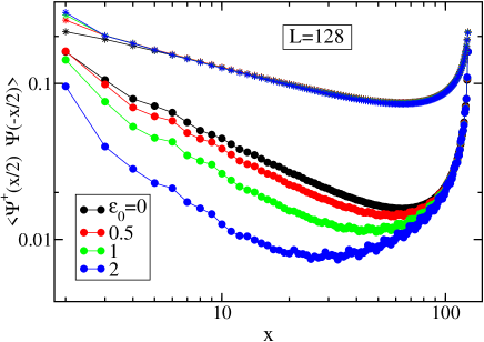
Figure 16: Impurity effect on the bosonic correlation function. For a relevant pin with $U=10$, $V=4$ and $g=0.72$ (circles) we find a strong suppression of correlations close to the impurity (which is at $x=0$). On the other hand, for an irrelevant pin with $U=5,V=0$, $g=1.41$ (stars) the dependence on the scattering potential $\epsilon_{0}$ is very weak. (These are the upper curves which lie almost on top of each other.)

Appendix D periodic/anti-periodic ground state energy difference

In this appendix we discuss the difference in ground state energies with anti-periodic and periodic boundary conditions on $\psi$. In the tight-binding model this corresponds to changing the sign of the hopping term on any single link. From Eq. (28) we see that anti-periodic boundary conditions on $\psi$,

$$\psi(x+L)=-\psi(x),$$ (206)

imply that the phase field $\phi$ must wind by a half-integer:

$$\phi(x+L)=\phi(x)+(2p+1)\pi,$$ (207)

for integer $p$. The ground states correspond to $\phi(x)=\pm\pi x/L$ with energy:

$$E^{AP}_{0}-E^{P}_{0}={\pi cg\over 2L}.$$ (208)

Upon noting that Eq. (208) determines $cg$ while the compressibility gives $g/c$, we see that both parameters are then determined.

The effects of a pin on the periodic/anti-periodic ground state energy difference can be calculated using “renormalization group improved” perturbation theory. Antiperiodic boundary conditions in the tight-binding model with a pin are defined by the Hamiltonian of Eq. (23) but with the periodic condition of eq. (24) replaced by:

$$b_{L}\equiv-b_{0}.$$ (209)

When the pin is irrelevant, $g>1$ and we expect to obtain the result of Eq. (208) asymptotically for large $L$. On the other hand, if the pin is relevant, $g<1$, the two sides of the system become asymptotically decoupled and this energy difference scales to zero more rapidly with $L$. Note that $E^{AP}_{0}-E^{P}_{0}$ is strictly zero at the open chain fixed point. Within the effective Hamiltonian of Eq. (127), we see that when $\Gamma=0$, it makes no difference whether we impose a boundary condition $\psi(0^{+})=\pm\psi(0^{-})$. For small $\Gamma$, this energy difference is first order in $\Gamma$. From Eq. (199), with $x$ and $y$ of order a short distance cut off, we obtain:

$$E_{0}^{AP}-E_{0}^{P}\propto{\Gamma\over L^{1/g}}.$$ (210)

If we now replace $\Gamma$ by its renormalized value at scale $L$, we obtain:

$$E_{0}^{AP}-E_{0}^{P}\propto{1\over L^{2/g-1}}.$$ (211)

Since $g<1$ here, we see that the decay is always faster than with no pin.

In fig. (17) we show numerical results for the boundary sensitivity $\Delta E_{0}\equiv E_{0}^{AP}-E_{0}^{P}$ normalized to the value without any defect. Although our system sizes were not big enough to extract power law behaviors, the data suggest that for a relevant pin ($g<1$) the normalized sensitivity decreases to zero in the thermodynamic limit, indicating that the system is indeed asymptotically “cut in two”. (For a very large system, we expect $\Delta E_{0}(\hbox{impurity}/\Delta E_{0}(\hbox{no impurity})\propto L^{2-2/g}$.) For $g>1$, on the other hand, our numerical results are consistent with a ratio which approaches unity for large $L$, indicating the irrelevance of the pin at large length scales.

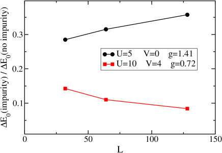
Figure 17: Sensitivity of the ground state energy to a change from periodic to antiperiodic boundary conditions for $n_{0}=0.25$ and $\epsilon_{0}=4$.

The Hamiltonian version of the $\phi$-representation is convenient for studying the periodic/anti-periodic ground state energy difference in the presence of a tilt field, $h$ (but no pin). [See Eqs. (21) and (46).] As discussed above Eq. (207), for anti-periodic boundary conditions, $\phi$ must wind by $\pm$ half a period in the ground state: $\phi(x)=\pm\pi x/L$. Note that the non-Hermitian term does not change the ground state but simply adds an imaginary term to its energy. We now have:

$$E_{0}^{AP}-E_{0}^{P}=\pm{ihn_{0}\pi\over m}+\pi cg/2L.$$ (212)

The imaginary term is $O(1)$, unlike the real term which is $O(1/L)$.

Appendix E Strength of point disorder

In this appendix we estimate the conditions such that the effect of residual point disorder on the thermally excited vortex lines, which are the main subject of this paper, can be ignored. This neglect can be justified only over a limited range of length scales. As discussed in Sec. 5, point disorder eventually changes the physics for any value of $g$. Our analysis is mostly based on Refs. (nelson92, ) and (Lehrer00, ), to which we refer readers for additional details.

The discussion proceeds in two stages. First, we demonstrate that in (1+1)–dimensional vortex arrays, typical pinning energies per unit length associated with an isolated columnar pin or “notch” greatly exceed the energy available from ignoring the pin and simply following an optimal path through the point disorder. Thus the columnar pinning energy greatly exceeds the collective effect of point pins. Second, given that at least one vortex line is strongly pinned on a columnar defect, we provide a rough estimate of a sufficient condition for thermal fluctuations of vortices to dominate over point disorder–induced wandering until one reaches the length scale of the renormalization group equations of Sec. 5. Our main conclusion is that (1+1)–dimensional “platelet” samples of high–$T_{c}$ materials (disordered only by oxygen vacancies) within 5-10% of the critical temperature could provide a good opportunity to study the physics of thermally excited vortex lines discussed in this paper over a range of length scales.

We first compute the average pinning energy of a single vortex, confined by its neighbors in a (1+1)–dimensional array, due to random point impurities. We define a characteristic “imaginary time” length scale $l^{*}$ at which transverse fluctuations of a vortex line due to point disorder reach the average vortex spacing $a_{0}$:

$$\delta x(l^{*})=x_{c}\left(\frac{l^{*}}{l_{c}}\right)^{\zeta}=a_{0}$$ (213)

where $\zeta=2/3$ in (1+1)–dimensionsLehrer00 and

$$x_{c}=T^{3}/\tilde{\epsilon}_{1}\tilde{\Delta}_{0},$$ (214)

$$l_{c}=\frac{\tilde{\epsilon}_{1}}{T}\,x^{2}_{c}.$$ (215)

Here $x_{c}$ is the length scale out to which vortex wandering is described by a thermal random walk, and $l_{c}<l^{*}$ is the corresponding length in the imaginary time direction. Note that $\tilde{\epsilon}_{1}$ is the line tension introduced in (2) and $\tilde{\Delta}_{0}$ is a correlator measuring the strength of point disorder. The parameter $\tilde{\Delta}_{0}$ is related to the correlator $\Delta_{0}$ introduced in the continuum model of Eq. (157) by $\tilde{\Delta}_{0}=\Delta_{0}/n_{0}^{2}$. The pinning energy for an imaginary–time segment of length $l$ on this path is given byLehrer00

$$U_{p}(l^{*})=T\left(\frac{l^{*}}{l_{c}}\right)^{2\zeta-1}.$$ (216)

Upon solving for $l^{*}$ and using $\zeta=2/3$ the pinning energy per length due to point disorder simplifies to:

$$\frac{U_{p}(l^{*})}{l^{*}}=\frac{\Delta_{0}}{a_{0}T}.$$ (217)

For quantitative estimates, we assume isotropy of the effective mass in the $ab$–plane and average over the sample thickness along the $c$–axis to obtain the disorder correlator asnelson92

$$\Delta_{0}=\frac{1}{w}\left(\frac{\phi_{0}}{4\pi\lambda}\right)^{4}\,\xi^{3}\,\left(\frac{J_{cp}}{J_{pb}}\right)^{3/2},$$ (218)

where $J_{pb}$ is the pair breaking critical current, $J_{cp}$ is the critical current due to point defects and $\phi_{0}=2\times 10^{-7}Gcm^{2}$ is the flux quantum. With sample thickness $w=150$ nm, penetration depth $\lambda=150$ nm, coherence length $\xi=2$ nm, temperature $T=50$ K, and the estimate (valid for high–$T_{c}$ superconductorsblatter94 ) $J_{cp}/J_{pb}\approx 0.01$, we obtain a pinning energy per length

$$\frac{U_{p}(l^{*})}{l^{*}}\approx 7\times 10^{-12}\hbox{erg/cm}.$$ (219)

For comparison, the pinning energy per unit length due to a columnar defect is given bynelson92

$$U_{0}/L=\left(\frac{\phi_{0}}{4\pi\lambda}\right)^{2}\approx 1.2\times 10^{-6}\hbox{erg/cm}$$ (220)

and is thus clearly dominant compared to point disorder by several orders of magnitude.

A related question concerns whether disorder affects the wandering of a single vortex line in (1+1)–dimensions before it interacts with its neighbors. Physically, we require that thermally excited vortices collide and restart their random walk several times before pinning due to point disorder becomes strong. Up to constants of order unity, the requirement is that the thermal length scale $x_{c}$ in Eq. (214) above exceed the vortex spacing $a_{0}$,

$$x_{c}=\frac{T^{3}}{\tilde{\epsilon}_{1}\Delta_{0}}>a_{0}$$ (221)

Using the same parameters as above, we find

$$x_{c}=3.5\times 10^{-7}cm$$ (222)

at $T=50K$. Upon assuming that $J_{cp}/J_{pb}$ is roughly temperature independent and noting that close to the critical temperature $\tilde{\epsilon}_{1}\Delta\propto\lambda^{-3}(T)\approx\lambda^{-3}(50K)|t|^{3/2}$ we have

$$\frac{T^{3}}{\tilde{\epsilon}_{1}\Delta}=\stackrel{{\scriptstyle\approx 3.5\times 10^{-6}cm}}{{\overbrace{\frac{T^{3}}{\tilde{\epsilon}_{1}\Delta}\Big{|}_{T=50K}}}}\,\left(\frac{T}{50K}\right)^{3}\,|t|^{-3/2}.$$ (223)

Here

$$t\equiv(T-T_{c})/T_{c}.$$ (224)

For a typical high-$T_{c}$ compound like YBCO with $T=80K$ and a reduced temperature $|t|=|T-T_{c}|/T_{c}=0.1$ we thus obtain

$$x_{c}\approx 2.7\times 10^{-5}cm>a_{0}$$ (225)

which is larger than a typical vortex spacing for $H\gtrsim\phi_{0}/(wx_{c})\approx 400G$. With these estimates in hand, we can use renormalization group recursion relations [see Sec. 5 and Ref. (polkovnikov, )] to determine the length scale at which point disorder dominates. For clean high $T_{c}$ samples close to the critical point, this length scale can be very large.

Appendix F Connection with string theory

The bosonized form of the weak tunnelling model, Eq. (127), generalized to arbitrary $g$, can be simplified by introducing linear combinations of the (independent) boson fields to the left and right of the pin:

$$\phi_{\pm}(x)\equiv[\phi(x)\pm\phi(L-x)]/\sqrt{2}.$$ (226)

Despite the non-local nature of this transformation, it yields a local Lagrangian since the interaction (tunneling) term occurs only at $x=0$. This Lagrangian takes the form:

$$L=\sum_{\pm}\int_{0}^{L/2}dx\left\{{g\over 2\pi}\left[{1\over c}\left({\partial\phi_{\pm}\over\partial\tau}\right)^{2}+c\left({\partial\phi_{\pm}\over\partial x}\right)^{2}\right]+{ihcg\sqrt{2}\over\pi}{\partial\phi_{-}\over\partial x}\right\}+\tilde{\Gamma}\cos[\sqrt{2}\phi_{-}(0)]$$ (227)

where $\tilde{\Gamma}\propto\Gamma$, the weak tunnelling amplitude introduced in Eq. (127). We see that $\phi_{+}$ decouples from both the pin and the tilt field. $\phi_{-}$ obeys mixed boundary conditions, $\phi_{-}(L/2)=0$, $d\phi_{-}/dx(0)=0$.

Alternatively, we may make the similarity transformation of Eq. (92) before rewriting the Lagrangian in terms of the phase field, $\phi$. This is equivalent to:

$$\phi(x)\to\phi(x)+ihx,$$ (228)

implying:

$$\phi_{-}(x)\to\phi_{-}(x)+ih(2x-L)/\sqrt{2}.$$ (229)

This eliminates the term proportional to $ih\partial\phi_{-}/\partial x$ but makes the tunnelling term non-Hermitian. Dropping the field $\phi_{+}$, we obtain the equivalent Lagrangian:

$$L={g\over 2\pi}\int_{0}^{L/2}dx\left[{1\over c}\left({\partial\phi_{-}\over\partial\tau}\right)^{2}+c\left({\partial\phi_{-}\over\partial x}\right)^{2}\right]+{\tilde{\Gamma}\over 2}\left[e^{hL}e^{i\sqrt{2}\phi_{-}(0)}+e^{-hL}e^{-i\sqrt{2}\phi_{-}(0)}\right].$$ (230)

In the small $\tilde{\Gamma}$ limit, it is permissible to drop the exponentially small term, $\propto\tilde{\Gamma}e^{-hL}$, leaving the Lagrangian:

$$L={g\over 2\pi}\int_{0}^{L/2}dx\left[{1\over c}\left({\partial\phi_{+}\over\partial\tau}\right)^{2}+c\left({\partial\phi_{+}\over\partial x}\right)^{2}\right]+{\tilde{\Gamma}\over 2}e^{hL}e^{i\sqrt{2}\phi_{-}(0)}.$$ (231)

Finally, if we make the formal analytic continuation, $\phi_{-}(x,\tau)\to-i\phi_{-}(x,\tau)$ we obtain:

$$L=-{g\over 2\pi}\int_{0}^{L/2}dx\left[{1\over c}\left({\partial\phi_{-}\over\partial\tau}\right)^{2}+c\left({\partial\phi_{-}\over\partial x}\right)^{2}\right]+{\tilde{\Gamma}\over 2}e^{hL}e^{\sqrt{2}\phi_{-}(0)}.$$ (232)

This is a strong coupling limit of a model, known as the time-like boundary Liouville theory, which has received considerable attention in the string theory literature lately (in the marginal case, $g=1$), because of its connection with “s-branes”, i.e. space-like “d-branes”. See, for example, Ref. (Gutperle, ).

References

- (1) D.J. Bishop, P.L. Gammel, D.A. Huse and C.A. Murray, Science 255, 165 (1992).
- (2) G. Blatter, M.V. Feigel’man, V.B. Geshkenbein, A.I. Larkin, and V.M. Vinokur, Rev. Mod Phys. 66, 1125 (1994).
- (3) U.C. Tauber and D.R. Nelson, Phys. Rep. 289, 157 (1997). See also, G. Crabtree and D.R. Nelson, Phys. Today, April, 1997.
- (4) T. Nattermann and S. Scheidl, Adv. Phys. 49, 607 (2000).
- (5) D.R. Nelson, Phys. Rev. Lett. 60, 1973 (1988); D.R. Nelson and H.S. Seung, Phys. Rev. B39, 9153 (1989).
- (6) M.P.A. Fisher, Phys. Rev. Lett. 62, 1415, (1989); D.S. Fisher, M.P.A. Fisher, and D.A. Huse, Phys. Rev. B43, 130 (1991).
- (7) D.R. Nelson and V.M. Vinokur, Phys. Rev. Lett. 68, 2398 (1992); Phys. Rev. B48, 13060 (1993).
- (8) T. Giamarchi and P. Le Doussal, Phys. Rev. Lett. 72, 1530 (1994); Phys. Rev. B52, 1242 (1995); see also T. Nattermann, Phys. Rev. Lett. 64, 2454 (1990).
- (9) M.P.A. Fisher and D.H. Lee, Phys. Rev. B39, 2756 (1989).
- (10) N. Hatano and D.R. Nelson, Phys Rev. Lett. 77, 570 (1996); Phys. Rev. B56, 8651 (1997); ibid, B58, 8384 (1998).
- (11) K.B. Efetov, Phys. Rev. Lett. 79, 491 (1997).
- (12) P.W. Brouwer, P.G. Silvestrov, and C.W.J. Beenakker, Phys. Rev. 56, R4333 (1997).
- (13) C. Mudry, P.W. Brouwer, B.I. Halperin, V. Gurarie and A. Zee, Phys. Rev. B58, 13 539 (1998).
- (14) V. Ta Phuoc, E. Olive, R. De Sousa, A. Ruyter, L. Ammor and J.C. Soret, Phys. Rev. Lett. 88, 187002 (2002).
- (15) T. Hwa, D.R. Nelson and V. Vinokur, Phys. Rev. B48, 1167 (1993). T.P. Devereau, R.T. Scalettar and G.T. Zimanyi, Phys Rev. B50, 13625 (1994).
- (16) R.A. Lehrer and D.R. Nelson, Phys. Rev. B58 12,385 (1998).
- (17) K. Kim and D.R. Nelson, Phys. Rev. B64, 054508 (2001).
- (18) L. Radzihovsky, Phys. Rev. Lett. 74, 4923 (1995).
- (19) E. Frey, D.R. Nelson and D.S. Fisher, Phys. Rev. B49 9723 (1994), and references therein.
- (20) C.A. Bolle, V. Aksyuk, F. Pardo, P.L. Gammel, E. Zeldov, E. Bucher, R. Boie, D.J. Bishop and D.R. Nelson, Nature 399, 43 (1999).
- (21) E. Zeldov, private communication.
- (22) H. Fukuyama and P.A. Lee, Phys Rev. B17, 535 (1977); P.A. Lee and T.M. Rice, Phys. Rev. B19, 3970 (1979).
- (23) F.D.M. Haldane, Phys. Rev. Lett. 47, 1840 (1981).
- (24) C.L. Kane and M.P.A. Fisher, Phys. Rev. Lett. 68, 1220 (1992); Phys. Rev. B46, 15233 (1992).
- (25) S. Eggert and I. Affleck, Phys. Rev. B46, 10866 (1992).
- (26) P.G. de Gennes, J. Chem. Phys. 48, 2257 (1968).
- (27) S.N. Coppersmith, D.S. Fisher, B.I. Halperin, P.A. Lee, and W.F. Brinkman, Phys. Rev. Lett. 46, 549 (1981); 46, 869(E); Phys. Rev. B 25, 349 (1982).
- (28) V.L. Pokrovskii and A.L. Talapov, Phys. Rev. Lett. 42, 65 (1979).
- (29) W. Hofstetter, I. Affleck, D.R. Nelson and U. Schollwöck, Europhys. Lett. 66, 178 (2004).
- (30) See, e.g., D.R. Nelson, in Phase Transitions and Critical Phenomena, Vol. 7, edited by C. Domb and J.L. Lebowitz (Academic Press, New York 1983).
- (31) S.R. White, Phys. Rev. Lett. 69, 2863 (1992), S.R. White, Phys. Rev. B 48, 10345 (1993).
- (32) I. Peschel, X. Wang, M. Kaulke and K. Hallberg (eds.), Density Matrix Renormalization, Springer (1999).
- (33) T. Nishino, J. Phys. Soc. Jpn. 64, 3598 (1995).
- (34) R.J. Bursill, T. Xiang and G.A. Gehring, J. Phys.: Condens. Matter 8, L583 (1996).
- (35) E. Carlon, M. Henkel and U. Schollwöck, Eur. J. Phys. B 12, 99 (1999).
- (36) G.H. Golub and C.F. van Loan, Matrix Computations (3rd ed.), Johns Hopkins Univ. Press (1996).
- (37) D. Day, SIAM, J. Matrix Anal. Appl. 18, 566 (1997).
- (38) T. Nishino and N. Shibata, J. Phys. Soc. Jpn. 68, 1537 (1999).
- (39) A. Kemper, A. Schadschneider and J. Zittartz, J. Phys. A: Math. Gen. 34, L279 (2001).
- (40) T. Enss and U. Schollwöck, J. Phys. A: Math. Gen. 34, 7769 (2001).
- (41) V. Meden, W. Metzner, U. Schollwöck and K. Schönhammer, Phys. Rev. B 65, 045318 (2002); V. Meden, W. Metzner, U. Schollwöck and K. Schönhammer, J. Low Temp. Phys. 126, 1147 (2002).
- (42) H.J. Schulz, B.I. Halperin and C.L. Henley, Phys. Rev. B 26, 3797 (1982).
- (43) D.R. Nelson in Phenomenology and Applications of High Temperature Superconductors, edited by K.S. Bedell et. al. (Addison Wesley, New York, 1991).
- (44) J. Jose, L. Kadanoff, S. Kirkpatrick and D.R. Nelson, Phys. Rev. B 16, 1217 (1977).
- (45) I. Affleck, in progress.
- (46) A. Gogolin and N. Prokof’ev, Phys. Rev. B50, 4921 (1994).
- (47) M. Fabrizio and A. Gogolin, Phys. Rev. B51, 17828 (1995); S. Eggert and I. Affleck, Phys. Rev. Lett. 75, 934 1995; R. Egger and H. Grabert, ibid, 3505.
- (48) A. Polkovnikov, Y. Kafri and D.R. Nelson (to be published).
- (49) T. Hwa and D.S. Fisher, Phys. Rev. Lett. 72, 2466 (1994).
- (50) J.L. Cardy and S. Ostlund, Phys. Rev. B 25, 6899 (1982).
- (51) J. Toner and D. DiVincenzo, Phys. Rev. B 41, 632 (1990).
- (52) See Appendix A of M. Rubinstein, B. Shraiman and D.R. Nelson, Phys. Rev. B 27, 1800 (1983).
- (53) J. Lou, S. Qin, T.-K. Ng, Z. Su and I. Affleck, Phys. Rev. B62, 3786 (2000).
- (54) E.H. Lieb and W. Liniger, Phys. Rev. 130, 1605 (1963); E.H. Lieb, ibid, 130, 1616 (1963).
- (55) I. Affleck, in preparation.
- (56) H.W.J. Blöte et al., Phys. Rev. Lett. 56, 742 (1986); I. Affleck, Phys. Rev. 56, 746 (1986).
- (57) T. Kühner et al., Phys. Rev. B61, 12474 (2000).
- (58) R.A. Lehrer and D.R. Nelson, Physica C 331, 317 (2000).
- (59) M. Gutperle and A. Strominger, Phys. Rev. D67, 126002 (2003).