Effects of Disorder on Coexistence and Competition between Superconducting and Insulating States

Abstract

We study effects of nonmagnetic impurities on the competition between the superconducting and electron-hole pairing. We show that disorder can result in coexistence of these two types of ordering in a uniform state, even when in clean materials they are mutually exclusive.

I Introduction

At low temperatures, many metals undergo a transition into a state with a gap in the single-electron excitation spectrum and become either superconductors or insulators with a periodic modulation of the electron charge or spin density. The insulating and superconducting (SC) orders inhibit each other by reducing the fraction of the Fermi surface available for the gap of the competing phase. The balance between the two phases is very sensitive to the Fermi surface shape and can be changed by, e.g., pressure, doping or magnetic field.

Nonetheless, in a surprisingly large number of materials the SC and insulating states coexist.Gabovich ; Gabovich2 This paper is focused on the coexistence of superconducting and charge density wave (CDW) states, observed in, e.g., layered transition metal dichalcogenides $2H$-NbSe₂ and $2H$-TaS₂,Wilson ; Jerome ; Berthier the quasi-one-dimensional compound NbSe₃,Fuller tungsten bronzes A_xWO₃,Stanley ; Cadwell and quarter-filled organic materials.Mori ; Merino One of the best studied and best characterized CDW superconductors is the transition metal dichalcogenide $2H$-NbSe₂. At $T_{d}=33.5$ K this compound undergoes a second-order phase transition to an incommensurate CDW state,moncton ; harper which is likely driven by the nesting of a part of the Fermi surface.straub ; Valla The resistivity, however, remains metallic-like down to $T_{c}=7.2$ K, at which this material becomes superconducting,Jerome ; Berthier and the superconductivity coexists with the CDW modulations.Du The coupling between the CDW and SC order parameters, resulting from the competition between these two states, was observed in a number of experiments. Thus, the suppression of the charge density modulation by pressure and hydrogen intercalation results in an increase of $T_{c}$.Berthier ; Monceau ; Murthy A similar interplay between the CDW and SC states upon applied pressure and doping is observed in NbSe₃ and tungsten bronzes.Fuller ; Stanley ; Cadwell

In this paper we adopt a rather general, though simplified, viewpoint on the interplay between the SC and CDW states. We assume that it originates from the competition between two different Fermi surface instabilities: the instability towards the electron pairing, which gives rise to superconductivity, and the instability towards the electron-hole (or excitonic) pairing. Here, we focus primarily on the effects of quenched disorder on this competition. We show that even in ‘the worst case scenario’, when the two states compete over the whole Fermi surface and therefore, in absence of disorder, are mutually exclusive, disorder stabilizes a uniform state, in which superconducting and insulating order parameters coexist. While having no effect on the superconducting phase, nonmagnetic disorder tends to close the CDW gap before completely suppressing the corresponding order parameter. Disorder induces low-energy states by breaking some of the electron-hole pairs. The released electrons and holes can subsequently form Cooper pairs, resulting in the coexistence of the two phases.

While in usual $s$-wave superconductors, non-magnetic impurities have little effect on the transition temperature,anderson experiments on electron irradiated transition metal dichalcogenides have shown strong dependence of $T_{c}$ on the concentration of defects.mutka This was attributed to the interplay between the SC and CDW orderings: Similarly to effect of pressure,Berthier ; Fuller disorder strongly suppresses the CDW state, which results in the observed increase of the SC critical temperature. Theoretically, the combined effect of the CDW modulation and disorder on the pairing instability have been studied in Ref. [Grest, ], where an increase of $T_{c}$ was found. However, in that paper the amplitude of the CDW modulation was assumed to be fixed, which is clearly insufficient in view of the strong suppression of the CDW state by disorder. In this paper we solve self-consistency equations for both SC and CDW order parameters, which allows us to study the interplay between these two different orders and obtain the temperature versus disorder phase diagram of CDW superconductors.

The remainder of the paper is organized as follows: In Sec. II we formulate an effective model describing the interplay between the superconducting and excitonic pairing. The self-consistency equations for the two order parameters are derived in Sec. III and in Sec. IV we analyze the phase diagram of the model. In Sec.V we discuss the electron-hole symmetry underlying the model and its consequences for the phase diagram. Finally, we conclude in Sec. VI. The details of the derivation of the effective model can be found in Appendix A.

II The model

In the following we consider the microscopic Hamiltonian

$$\hat{\mathcal{H}}=\int d\mathbf{x}\left\{\sum_{\sigma}\sum_{j=a,b}\psi_{j\sigma}^{{\dagger}}\left[\varepsilon_{j}(-i\nabla_{\mathbf{x}})+U(\mathbf{x})\right]\psi_{j\sigma}\right.\\ \left.-g_{1}\left(\psi_{a\uparrow}^{{\dagger}}\psi_{a\uparrow}\psi_{a\downarrow}^{{\dagger}}\psi_{a\downarrow}+\psi_{b\uparrow}^{{\dagger}}\psi_{b\uparrow}\psi_{b\downarrow}^{{\dagger}}\psi_{b\downarrow}\right)\right.\\ \left.+g_{2}\sum_{\sigma\sigma^{\prime}}\psi_{a\sigma}^{{\dagger}}\psi_{a\sigma}\psi_{b\sigma^{\prime}}^{{\dagger}}\psi_{b\sigma^{\prime}}\right\}$$ (1)

describing two types of fermions, one with hole-like dispersion ($a$-electrons) and another with electron-like dispersion ($b$-electrons), $\varepsilon_{j=a,b}(\mathbf{k})=\pm(k_{F}^{2}-\mathbf{k}^{2})/2m$ ($\hbar=1$), where $\mu=k_{F}^{2}/2m$ denotes the chemical potential (see Fig. 1). Here, in comparison with the models generally used to represent CDW systems, two nested parts of a single Fermi surface are replaced by two spherical Fermi surfaces matching at the Fermi wave vector $k_{F}$. The excitonic insulator (EI) state is the condensate of pairs formed by $b$-electrons and $a$-holes (or vice versa) with the zero total momentum.Keldysh It is an analogue of the condensate of electron-hole pairs with the total momentum $\hbar{\bf Q}$, where Q is a nesting wave vector, appearing in the CDW state.

The disorder potential $U(\mathbf{x})$ encapsulates the effect of non-magnetic impurities in the system. Here, we assume that the latter is drawn at random from a Gaussian distribution with zero mean and variance given by

$$\langle U(\mathbf{x})U(\mathbf{y})\rangle=\frac{\Gamma}{2\pi\nu_{F}}\delta(\mathbf{x-y})\;,$$ (2)

where $\Gamma$ is the inverse scattering time and $\nu_{F}=mk_{F}/2\pi^{2}$ is the density of states at the Fermi energy. For simplicity we have assumed the electron and hole effective masses to be equal.

The interaction term characterized by the coupling strength $g_{1}$ describes the attraction between electrons of the same type (e.g. due to the phonon-exchange), while the $g_{2}$ term describes the (Coulomb) repulsion between the $a$- and $b$-electrons ($g_{1},g_{2}>0$). The attraction between electrons favors $s$-wave superconductivity, while the second interaction leads to an attraction between electrons and holes and vice versa, favoring the EI state. Here, we neglect the inter-band electron transitions due to scattering off impurities and electron-electron interactions, so that the numbers of the $a$- and $b$-electrons are separately conserved and fixed by the chemical potential. Such terms will formally destroy long-range order of the EI phase, corresponding to the suppression of the long-ranged CDW order, due to the pinning of the CDW phase by randomly distributed impurities. However, for the essentially short-length-scale physics we shall discuss, these effects may be neglected. In the absence of disorder, the same model (1) has been employed to study the competition between SC and EI states for an arbitrary ratio of electron and hole densities.Rusinov The effect of disorder on the EI state alone has been considered in the seminal work of Ref. [Zittartz, ], where the analogy of the problem to an $s$-wave superconductor in presence of magnetic impuritiesAbrikosovGorkov was drawn.

Figure 1: Schematic picture of the hole-like ($a$) and electron-like ($b$) bands.

The particular fermion-fermion interactions considered in (1) – attraction between electrons of the same type and repulsion between the $a$- and $b$-electrons – open the possibility to have simultaneously both superconducting and insulating instabilities. A more realistic starting point would be a model with attractive phonon-mediated interactions and Coulomb repulsion between all types of electrons. However, it is possible to demonstrate that, since the former are retarded, while the latter is practically instantaneous, the SC and EI order parameters turn out to have a very different dependence on the Matsubara frequency $\omega$. This is clearly shown in Fig. 2: The SC order parameter is large at small frequencies, while at higher values, it decreases in magnitude and finally changes sign when $\omega$ is of the order of the phonon frequency $\Omega_{0}$.AndersonMorel By contrast, the EI parameter is large at high frequencies and has a dip for $|\omega|<\Omega_{0}$. In other words, the difference in frequency scales of the attractive and repulsive interactions allows both instabilities to be present simultaneously. Furthermore, in the weak coupling limit and for a weak disorder, i.e. $\Gamma\ll\Omega_{0}$, the frequency dependence of the two order parameters can be found separately for $\omega\sim\Gamma$ and $\omega\gtrsim\Omega_{0}$. Furthermore, it can be shown that the self-consistency equations for the order parameters at $\omega=0$ coincide with the ones obtained from the model (1), which therefore can be interpreted as an effective interacting model. Technical details together with the frequency dependence of the two order parameters and the explicit expressions for the coupling constants $g_{1}$ and $g_{2}$ in terms of the Coulomb and electron-phonon couplings can be found in appendix A.

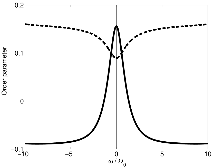
Figure 2: The dependence of the superconducting (solid line) and excitonic (dashed line) order parameters on the Matsubara frequency $\omega$ (see appendix A for details).

III Order parameters and self-consistency equations

Four order parameters describing the SC and EI states can be introduced by means of the following anomalous averages

$$\Delta_{1a} =g_{1}\langle\psi_{a\uparrow}\psi_{a\downarrow}\rangle \Delta_{1b} =g_{1}\langle\psi_{b\uparrow}\psi_{b\downarrow}\rangle$$

$$\Delta_{2\uparrow} =-g_{2}\langle\psi_{a\uparrow}^{{\dagger}}\psi_{b\uparrow}\rangle \Delta_{2\downarrow} =-g_{2}\langle\psi_{a\downarrow}^{{\dagger}}\psi_{b\downarrow}\rangle\;.$$

Since the numbers of the $a$- and $b$-fermions are separately conserved, for homogeneous states, we use the global gauge transformation

$$\psi_{a} \mapsto e^{i\varphi_{a}}\psi_{a} \psi_{b} \mapsto e^{i\varphi_{b}}\psi_{b}\;,$$

to make the SC order parameters, $\Delta_{1a}$ and $\Delta_{1b}$, real and positive. Moreover, as electrons and holes are characterized by the same dispersion, we can require, without a loss of generality, that

$$\Delta_{1a}=\Delta_{1b}=\Delta_{1}>0\;.$$

In case of a spin-independent interaction, as in (1), singlet and triplet exciton pairs are degenerate in energy. This gives rise to a large symmetry class of transformations for the EI order parameter $\Delta_{2\sigma}$. In reality, however, this degeneracy is lifted by Coulomb exchange interactions and inter-band transitions. Therefore, we will assume the exciton pairs have zero total spin, i.e. $\Delta_{2\uparrow}=\Delta_{2\downarrow}=\Delta_{2}$.

Finally we note that, when $\Delta_{1},\Delta_{2}\neq 0$ and $\Delta_{2}$ has an imaginary part, a pairing of electrons of different types, $\Delta_{1ab}=-g_{2}\langle\psi_{a\uparrow}\psi_{b\downarrow}\rangle=-g_{2}\langle\psi_{b\uparrow}\psi_{a\downarrow}\rangle$, may be present.Rusinov However, one can show the energy of the state with coexisting SC and EI orders to be the lowest for real $\Delta_{2}$, in which case $\Delta_{1ab}=0$.

By analogy with the case of magnetic impurities in $s$-wave superconductors,AbrikosovGorkov restricting attention to the limit in which the disorder potential imposes only a weak perturbation on the electronic degrees of freedom ($\mu\ll\Gamma$), the mean field (saddle-point) equations together with the self-consistency equations for the EI and SC order parameters can be obtained using the diagrammatic technique. However, we will find it more convenient to use a path-integral approach. This will also allows us to obtain straightforwardly an expression for the average free energy.

The quantum partition function, $\mathcal{Z}=\rm{tr}[e^{-\beta\hat{\mathcal{H}}}]$, where $\beta=1/T$, can be expressed as a coherent state path integral over fermionic fields. In order to facilitate the averaging of the free energy over the disorder potential (2), it is convenient engage the replica trick:edwards_anderson

$$F=-\frac{1}{\beta}\langle\ln\mathcal{Z}\rangle=-\frac{1}{\beta}\lim_{n\to 0}\frac{\langle\mathcal{Z}^{n}\rangle-1}{n}\;.$$

Once replicated, a Hubbard-Stratonovich transformation can be applied to decouple the interaction terms in the Hamiltonian. As a result, one obtains:

$$\mathcal{Z}^{n}=\int D(\Psi,\Psi^{\dagger})\int D\Delta_{1}D\Delta_{2}\\ \exp\left\{\int_{0}^{\beta}d\tau\int d\mathbf{x}\left[\Psi^{\dagger}\left(\partial_{\tau}+\hat{H}\right)\Psi+2\frac{\Delta_{1}^{2}}{g_{1}}+2\frac{\Delta_{2}^{2}}{g_{2}}\right]\right\}\;.$$

Here, omitting the replica indices for clarity, the fermion field is arranged in a Nambu-like spinor, $\Psi^{\rm T}=(\psi_{b\uparrow},\psi_{a\uparrow},\psi_{b\downarrow}^{\dagger},\psi_{a\downarrow}^{\dagger})$, in such a way the single quasi-particle Hamiltonian takes the following form:

$$\hat{H}=\hat{\xi}_{\hat{\mathbf{p}}}\tau_{3}\sigma_{3}+U(\mathbf{x})\tau_{3}+\Delta_{1}\tau_{1}+\Delta_{2}\tau_{3}\sigma_{1}\;,$$ (3)

where, $\hat{\xi}_{\hat{\mathbf{p}}}=-\nabla^{2}_{\mathbf{x}}/2m-\mu$ and the Pauli matrices $\tau_{c}$ and $\sigma_{c}$ ($c=1,2,3$) act, respectively, in the particle-hole and the $b,a$ subspace.

The ensemble average over the quenched random potential distribution (2) induces a time non-local quartic interactions, $\int d\mathbf{x}(\int_{0}^{\beta}d\tau\Psi^{\dagger}\tau_{3}\Psi)^{2}$, which can be decoupled by means of a Hubbard-Stratonovich transformation with the introduction of a matrix field, $\Sigma(\mathbf{x})$, local in real space, and carrying replica, Matsubara ($\omega_{n}=(2n+1)\pi/\beta$) and internal (particle-hole and $b,a$) indices. Integrating over the Fermionic fields $\Psi$, one obtains the ensemble averaged replicated partition function:

$$\langle\mathcal{Z}^{n}\rangle=\int D\Delta_{1}D\Delta_{2}\int D\Sigma e^{-\beta F}\;,$$

where $F$ is the free energy of the system

$$\beta F=\int_{0}^{\beta}d\tau\int d\mathbf{x}\left(2\frac{\Delta_{1}^{2}}{g_{1}}+2\frac{\Delta_{2}^{2}}{g_{2}}\right)\\ -\rm{tr}\ln\left(-\hat{\mathcal{G}}^{-1}\right)-\frac{\pi\nu_{F}}{\Gamma}\int d\mathbf{x}\,\rm{tr}\left[\Sigma(\mathbf{x})\tau_{3}\right]^{2}$$ (4)

and $\hat{\mathcal{G}}$ is the quasi-particle matrix Green function in the presence of disorder:

$$-\hat{\mathcal{G}}^{-1}=-i\omega_{n}+\hat{\xi}_{\hat{\mathbf{p}}}\tau_{3}\sigma_{3}+\Delta_{1}\tau_{1}+\Delta_{2}\tau_{3}\sigma_{1}+\Sigma(\mathbf{x})\;.$$ (5)

The matrix field $\Sigma(\mathbf{x})$ represents the contribution of the non-magnetic impurity interaction to the self-energy.

The saddle-point associated with the action (4) obtained by variation with respect to the self-energy $\Sigma$,

$$\Sigma(\mathbf{x})=\frac{\Gamma}{2\pi\nu_{F}}\tau_{3}\langle\mathbf{x}|\hat{\mathcal{G}}|\mathbf{x}\rangle\tau_{3}\;,$$

can be solved in the limit $\mu\gg\Gamma,\Delta_{1},\Delta_{2}$, when $\Sigma$, $\Delta_{1}$ and $\Delta_{2}$ can be considered homogeneous. In this limit, which is compatible with the self-consistent Born approximation, the Green function (5) is diagonal in frequency and momentum space and can be explicitly inverted:

$$\mathcal{G}_{\omega_{n},\mathbf{p}}=-\frac{i\tilde{\omega}_{n}+\xi_{\mathbf{p}}\tau_{3}\sigma_{3}+\tilde{\Delta}_{1}\tau_{1}+\tilde{\Delta}_{2}\tau_{3}\sigma_{1}}{\tilde{\omega}_{n}^{2}+\xi_{\mathbf{p}}^{2}+\tilde{\Delta}_{1}^{2}+\tilde{\Delta}_{2}^{2}}\;.$$

Here, we have defined the ‘renormalized’ expressions for the frequency and order parameters:

$$\begin{split}\displaystyle\tilde{\omega}_{n}\left(1-\frac{\Gamma}{2}\frac{1}{\sqrt{\tilde{\omega}_{n}^{2}+\tilde{\Delta}_{1}^{2}+\tilde{\Delta}_{2}^{2}}}\right)&=\omega_{n}\\ \tilde{\Delta}_{1}\left(1-\frac{\Gamma}{2}\frac{1}{\sqrt{\tilde{\omega}_{n}^{2}+\tilde{\Delta}_{1}^{2}+\tilde{\Delta}_{2}^{2}}}\right)&=\Delta_{1}\\ \tilde{\Delta}_{2}\left(1+\frac{\Gamma}{2}\frac{1}{\sqrt{\tilde{\omega}_{n}^{2}+\tilde{\Delta}_{1}^{2}+\tilde{\Delta}_{2}^{2}}}\right)&=\Delta_{2}\;.\end{split}$$ (6)

From the above equations of motion, one may deduce that

$$\frac{\tilde{\omega}_{n}}{\tilde{\Delta}_{1}}=\frac{\omega_{n}}{\Delta_{1}}\;,$$ (7)

or, in other words, that in the weak disorder limit non magnetic impurities do not suppress $s$-wave superconductivity (Anderson theorem,anderson ) while, introducing the parameters $u=\tilde{\omega}_{n}/\tilde{\Delta}_{2}$ and $\zeta=\Gamma/\tilde{\Delta}_{2}$,

$$\frac{\omega_{n}}{\Delta_{2}}=u\left[1-\frac{\zeta}{\sqrt{1+u^{2}\left(1+\Delta_{1}^{2}/\omega_{n}^{2}\right)}}\right]\;.$$ (8)

Finally, the self-consistency equations for the SC and EI order parameters can be found minimizing the action (4) with respect to $\Delta_{1,2}$:

$$\Delta_{1,2}=\frac{\pi\lambda_{1,2}}{\beta}\sum_{\omega_{n}}\frac{\tilde{\Delta}_{1,2}}{\sqrt{\tilde{\omega}_{n}^{2}+\tilde{\Delta}_{1}^{2}+\tilde{\Delta}_{2}^{2}}}\;.$$ (9)

Here, $\lambda_{1,2}=g_{1,2}\nu_{F}$ represent dimensionless coupling constants. Note that, as in conventional BCS theory, the integral over momentum can be performed by making use of the identity $\int d\mathbf{p}/(2\pi)^{3}=\int d\xi\nu(\xi)\simeq\nu_{F}\int d\xi$. Employing Eq. (8), the self-consistency equations can then be rewritten in the form

$$\begin{split}\displaystyle\frac{1}{\lambda_{1}}&=\frac{\pi}{\beta}\sum_{\omega_{n}}\left[\Delta_{1}^{2}+\omega_{n}^{2}\left(1+\frac{1}{u^{2}}\right)\right]^{-1/2}\\ \displaystyle\Delta_{2}&=\frac{\lambda_{2}\pi}{\beta}\sum_{\omega_{n}}\left[1+u^{2}\left(1+\frac{\Delta_{1}^{2}}{\omega_{n}^{2}}\right)\right]^{-1/2}\;.\end{split}$$ (10)

Combining together equations (6) with (10), we are now able to discuss the finite and zero temperature mean-field phase diagram associated with the model (1).

IV Phase diagram

IV.1 Temperature versus disorder phase diagram

In the absence of disorder (i.e. $\Gamma=0$ and $u=\omega_{n}/\Delta_{2}$), one may note that, except for different coupling constants, the two self-consistency equations (10) are identical. Therefore, since they cannot be satisfied simultaneously, even though the SC and EI instabilities can occur simultaneously, in clean materials the corresponding orderings are mutually exclusive. For $\lambda_{1}>\lambda_{2}$ the system becomes superconducting below

$$T_{1}(\Gamma=0)=\frac{\gamma_{E}}{\pi}2\Omega_{0}\,e^{-1/\lambda_{1}}\;,$$ (11)

where $\Omega_{0}$ is the frequency cutoff and $\gamma_{E}\simeq 1.78$ is the Euler constant while, for $\lambda_{2}>\lambda_{1}$, the transition into the EI state occurs at

$$T_{2}(\Gamma=0)=\frac{\gamma_{E}}{\pi}2\Omega_{0}\,e^{-1/\lambda_{2}}\;.$$ (12)

Since charged non-magnetic impurities act as electron-hole pair breaking perturbations, while they do not affect the SC state, for $\lambda_{1}>\lambda_{2}$ the SC state dominates at any disorder strength $\Gamma$ and the EI state never appears. On the other hand, for $\lambda_{2}>\lambda_{1}$, the EI phase is energetically more favorable at weak disorder, becomes suppressed for larger values of $\Gamma$, and eventually gives way to superconductivity. Non-magnetic impurities suppress the EI state in exactly the same way as magnetic impurities suppress the SC state.AbrikosovGorkov ; Zittartz Therefore, one can infer that the dependence of the EI transition temperature $T_{2}$ on the disorder strength $\Gamma$ is described by the standard Abrikosov-Gor’kov expression:

$$\ln\frac{T_{2}(0)}{T_{2}(\Gamma)}=\Psi\left(\frac{1}{2}+\frac{\Gamma}{2\pi T_{2}(\Gamma)}\right)-\Psi\left(\frac{1}{2}\right)\;.$$ (13)

At some critical disorder strength $\Gamma_{\ast}$, the EI and SC transition temperatures eventually coincide $T_{2}(\Gamma_{\ast})=T_{1}(\Gamma=0)=T_{\ast}$ and, for $\Gamma>\Gamma_{\ast}$, the system becomes superconducting at the ($\Gamma$-independent) temperature $T_{1}$ given by Eq. (11).

One can therefore wonder in what way, at temperatures lower than $T_{\ast}$, the transition between the EI and SC states takes place. In Fig. 3, the temperature versus disorder phase diagram is shown for values of the coupling constants such that $\eta=\lambda_{1}^{-1}-\lambda_{2}^{-1}=0.5$. The pure EI and SC states are separated by a very thin region located in the $\Gamma<\Gamma_{\ast}$ and $T<T_{\ast}$ region of the phase diagram, where the two order parameters coexist. The three ordered phases (EI, SC, and EI+SC) and the high-temperature disordered phase merge at the tetracritical point $(\Gamma_{\ast},T_{\ast})$. The boundaries between the coexistence region and the two pure phases are critical lines of second order transitions although, due to the very small width of the coexistence region, the evolution of one pure phase into another is close to being of first-order. This will be further discussed in Sec. V.

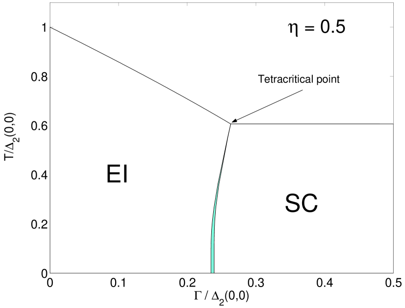
Figure 3: The temperature vs disorder strength phase diagram of the model Eq.(1) for $\lambda_{1}^{-1}-\lambda_{2}^{-1}=0.5$ . The dimensionless disorder strength is $\Gamma/\Delta_{2}(T=0,\Gamma=0)$ and temperature is measured in units of $T_{c2}(\Gamma=0)$. The EI and SC state are separated by a thin domain, in which the two order parameters coexist.

At the first critical line $T_{1}(\Gamma)$ separating the pure EI phase from the mixed EI+SC phase, one has $\Delta_{1}\to 0$ and $\Delta_{2}\neq 0$. In the $\Delta_{1}\to 0$ limit, the self-consistency equations (10) simplify to the expressions

$$\begin{split}\displaystyle\frac{1}{\lambda_{1}}&=2\pi T_{1}\sum_{\omega_{n}>0}\frac{u}{\omega_{n}\sqrt{1+u^{2}}}\\ \displaystyle\frac{\Delta_{2}}{\lambda_{2}}&=2\pi T_{1}\sum_{\omega_{n}>0}\frac{1}{\sqrt{1+u^{2}}}\;.\end{split}$$ (14)

The second critical line $T_{2}(\Gamma)$ separates the mixed state from the pure SC state and is obtained by instead taking the limit $\Delta_{2}\to 0$ for nonzero $\Delta_{1}$. In this case, one can approximate

$$u\simeq\frac{\omega_{n}}{\Delta_{2}}\left(1+\frac{\Gamma}{\sqrt{\omega_{n}^{2}+\Delta_{1}^{2}}}\right)\;,$$

whereupon Eqs. (10) take the form

$$\begin{split}\displaystyle\frac{1}{\lambda_{1}}&=2\pi T_{2}\sum_{\omega_{n}>0}\frac{1}{\sqrt{\omega_{n}^{2}+\Delta_{1}^{2}}}\\ \displaystyle\frac{1}{\lambda_{2}}&=2\pi T_{2}\sum_{\omega_{n}>0}\frac{1}{\sqrt{\omega_{n}^{2}+\Delta_{1}^{2}}+\Gamma}\;.\end{split}$$ (15)

Note that the EI order parameter $\Delta_{2}$ appears at temperatures lower than the “upper” $T_{2}(\Gamma)$ given by Eq.(13), and disappears below the “lower” $T_{2}(\Gamma)$, given by Eq. (15). Figure 3 shows that $\Gamma_{1}$ (at which the SC ordering sets in at $T=0$) and $\Gamma_{2}$ (at which the EI ordering is destroyed at $T=0$) are smaller than the disorder strength at the tetracritical point $\Gamma_{\ast}$. Therefore, in the interval $\Gamma_{2}<\Gamma<\Gamma_{\ast}$, the system passes through three consecutive phase transitions as the temperature decreases: Firstly the system becomes an excitonic insulator, then it enters the mixed phase with the two coexisting order parameters, and finally the growth of the SC order parameter with decreasing temperature suppresses the EI ordering, resulting in the transition into the pure SC state with $\Delta_{2}=0$.

IV.2 The zero temperature phase diagram

The zero temperature phase diagram is shown in Fig. 4. The EI state exists only for positive $\eta$ (or equivalently $e^{-\eta}=\Delta_{1}(T=0)/\Delta_{2}(T=0,\Gamma=0)<1$). The coexistence region (shaded) is confined between the two critical lines $\Gamma_{1}(\eta)<\Gamma_{2}(\eta)$. The system is superconducting for $\Gamma>\Gamma_{1}$, while the excitonic condensate appears for $\Gamma<\Gamma_{2})$. For small $\eta$, i.e. close to the quantum critical point separating the EI and SC states in the absence of disorder, the critical disorder values can be obtained as

$$\begin{array}[]{cl}\gamma_{1}(\eta)&\simeq\frac{2}{\pi}\eta-\frac{3\pi^{2}+8}{3\pi^{3}}\eta^{2},\\ \\ \gamma_{2}(\eta)&\simeq\frac{2}{\pi}\eta-\frac{2\pi^{2}-8}{\pi^{3}}\eta^{2}\;,\end{array}$$ (16)

where $\gamma\equiv\Gamma/\Delta_{2}(0,0)$. Therefore, the width of the coexistence region is approximately given by $\gamma_{2}-\gamma_{1}\simeq 0.08\eta^{2}$.

For large values of $\eta$, i.e. when the SC coupling $\lambda_{1}$ is much smaller than the EI coupling $\lambda_{2}$, the coexistence region essentially coincides with the disorder interval $e^{-\pi/4}<\gamma<1/2$ in which the EI state is gapless.AbrikosovGorkov ; Zittartz Therefore, for $\eta>1+3\pi/4$, the superconductivity appears at the same disorder value, at which the EI becomes gapless, $\gamma_{1}=e^{-\pi/4}\simeq 0.46$, while $\Gamma_{2}$ asymptotically approaches the disorder strength at which the EI state is destroyed in the absence of superconductivity:

$$\gamma_{2}\simeq 1/2-\eta e^{-2\eta^{2}}\qquad\eta\gg 1\;.$$ (17)

We note that, for $\eta<1+3\pi/4$, the gap in the spectrum of quasi-particle excitations at zero temperature is nonzero for all $\Gamma$, while for $\eta>1+3\pi/4$ it vanishes at a single point $\Gamma=\Gamma_{1}$.

This re-entrant behavior and the form of the phase diagram are similar to what was found for the spin-Peierls compound CuGeO₃ , which upon doping shows an antiferromagnetic ordering coexisting with spin-Peierls phase in some interval of doping concentrations.MKK ; Kiryukhin

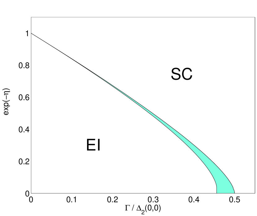
Figure 4: The zero temperature phase diagram. Close to the quantum critical point $\eta=\Gamma=0$, the coexistence region is extremely thin. For $\eta\ll 1$ it practically coincides with the disorder interval, in which the EI is gapless.

V EI-SC symmetry

To understand why the coexistence region is so narrow, it is instructive to plot the EI and SC order parameters as functions of $\Gamma$ in the coexistence region (see Fig. 5). In the interval $\Gamma_{1}<\Gamma<\Gamma_{2}$ the excitonic(superconducting) order parameter decreases (increases) fast with increasing $\Gamma$, while $\Delta=\sqrt{\Delta_{1}^{2}+\Delta_{2}^{2}}$ stays approximately constant.

This behavior results from the symmetry between the $b$- and $a$-electrons at the quantum critical point $\lambda_{1}=\lambda_{2}$ in the absence of disorder ($\Gamma=0$):

$$\Psi\mapsto e^{i\phi\tau_{2}\sigma_{1}/2}\Psi\;.$$ (18)

This transformation results is the rotation in the space of the two order parameters over the angle $\phi\in[0,2\pi]$,

$$\Delta_{1} \mapsto\Delta_{1}\cos\phi-\Delta_{2}\sin\phi$$

$$\Delta_{2} \mapsto\Delta_{2}\cos\phi+\Delta_{1}\sin\phi\;.$$

At the mean-field level, the anomalous part of the average free energy per unity of volume, $\langle f\rangle=\langle F\rangle/V$, can be easily evaluated starting from (4) and making use of the replica trick:

$$\langle f\rangle=-\frac{4\pi}{\beta}\sum_{\omega_{n}}\left(\sqrt{\tilde{\omega}_{n}^{2}+\tilde{\Delta}_{1}^{2}+\tilde{\Delta}_{2}^{2}}-\left|\tilde{\omega}_{n}+\rm{sign}(\tilde{\omega}_{n})\frac{\Gamma}{2}\right|\right)\\ -\frac{2\pi\Gamma}{\beta}\sum_{\omega_{n}}\frac{\tilde{\Delta}_{2}^{2}}{\tilde{\omega}_{n}^{2}+\tilde{\Delta}_{1}^{2}+\tilde{\Delta}_{2}^{2}}+\frac{2}{\lambda_{1}}\Delta_{1}^{2}+\frac{2}{\lambda_{2}}\Delta_{2}^{2}\;.$$ (19)

Let us notice that, in the absence of disorder, the free energy only depends on ‘the total gap’ $\Delta=\sqrt{\Delta_{1}^{2}+\Delta_{2}^{2}}$. This follows from the fact that the generator of the EI-SC rotations $\tau_{2}\sigma_{1}$ commutes with the Hamiltonian Eq. (3) for $U(\mathbf{x})=0$. Moreover, for $g_{1}=g_{2}$, the last term in Eq. (19) is equal to $2\Delta^{2}/g_{1}$ (the second term in Eq. (19) vanishes for $\Gamma=0$). Thus, at the quantum critical point the free energy has a ‘Mexican hat’ profile as a function of the order parameters $(\Delta_{1},\Delta_{2})$, symmetric under the rotations transforming the excitonic insulator into the superconductor. This symmetry between electron-electron and electron-hole pairing is analogous to the symmetry unifying the $d$-wave superconductivity and antiferromagnetism discussed in the context of high-T_c and heavy fermion materials.solomon ; Zhang ; Kitaoka

Away from the quantum critical point, and for nonzero disorder, the electron-hole symmetry is broken. Solving Eqs. (6) for $\tilde{\omega}_{n}$, $\tilde{\Delta}_{1}$, and $\tilde{\Delta}_{2}$, perturbatively in the disorder strength $\Gamma$, and replacing at $T=0$ the summations over the Matsubara frequency $\omega_{n}$ in Eq. (19) by integrals, one can obtain an expansion of the average energy density in powers of $\Gamma$:

$$\frac{\langle f\rangle}{2\nu_{F}}=\frac{\Delta_{1}^{2}}{\lambda_{1}}+\frac{\Delta_{2}^{2}}{\lambda_{2}}-\Delta^{2}\,\ln\left(2\frac{\Omega_{0}}{\Delta}\right)-\frac{1}{2}\Delta^{2}\\ +\frac{\pi}{2}\frac{\Delta_{2}^{2}}{\Delta}\Gamma-\frac{1}{3}\frac{\Delta_{2}^{2}(3\Delta_{1}^{2}+\Delta_{2}^{2})}{\Delta^{4}}\Gamma^{2}\\ -\frac{\pi}{16}\frac{\Delta_{1}^{2}\Delta_{2}^{2}(\Delta_{2}^{2}-4\Delta_{1}^{2})}{\Delta^{7}}\Gamma^{3}+O\left(\Gamma^{4}\right)\;.$$ (20)

Denoting the dimensionless disorder strength by $\delta=\Gamma/\Delta\ll 1$ and defining the angle $\phi$

$$\Delta_{1} =\Delta\cos\phi \Delta_{2} =\Delta\sin\phi\;,$$

we can recast Eq. (20) in the form

$$\frac{\langle f\rangle}{2\nu_{F}}\simeq\Delta^{2}\left[\ln\frac{\Delta}{{\bar{\Delta}}}-\frac{1}{2}+\frac{\eta}{2}\cos 2\phi+\frac{\pi\delta}{4}\left(1-\cos 2\phi\right)\right.\\ \left.-\frac{\delta^{2}}{12}\left(3-2\cos 2\phi-\cos 4\phi\right)\right.\\ \left.+\frac{\pi\delta^{3}}{512}\left(6+5\cos 2\phi-6\cos 4\phi-5\cos 6\phi\right)+O\left(\delta^{4}\right)\right]\;,$$ (21)

where ${\bar{\Delta}}$ is the geometric mean of the EI and SC order parameters, $\bar{\Delta}=\sqrt{\Delta_{1}\Delta_{2}(0,0)}=2\Omega_{0}e^{-(\lambda_{1}^{-1}+\lambda_{2}^{-1})/2}$. The symmetry-breaking terms in Eq. (21) (that depend on the angle $\phi$) are proportional to powers of $\eta$ and $\delta$. Thus, for $\eta,\delta\ll 1$, these terms are small and the energy has the slightly deformed ‘Mexican hat’ shape with an almost flat valley connecting the points $\Delta_{\text{min}}(\phi)$, at which $\langle f\rangle$ has a minimum for a given $\phi$.

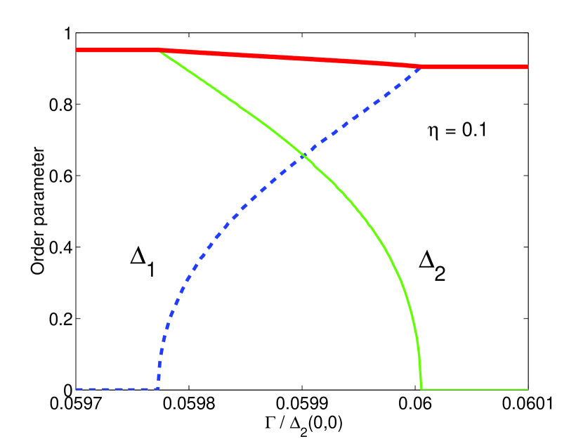
Figure 5: The plots shows the dependence of the superconducting order parameter $\Delta_{1}$ (dashed line) and the excitonic order parameter $\Delta_{2}$ (thin solid line) on the disorder strength $\Gamma$ in the region of coexistence of the two phases for $\eta=0.1$ and $T=0$. For $\Gamma_{1}<\Gamma<\Gamma_{2}$, $\Delta_{1}$ and $\Delta_{2}$ vary very fast, while $\Delta=\sqrt{{\Delta_{1}}^{2}+{\Delta_{2}}^{2}}$ (thick line) stays approximately constant.

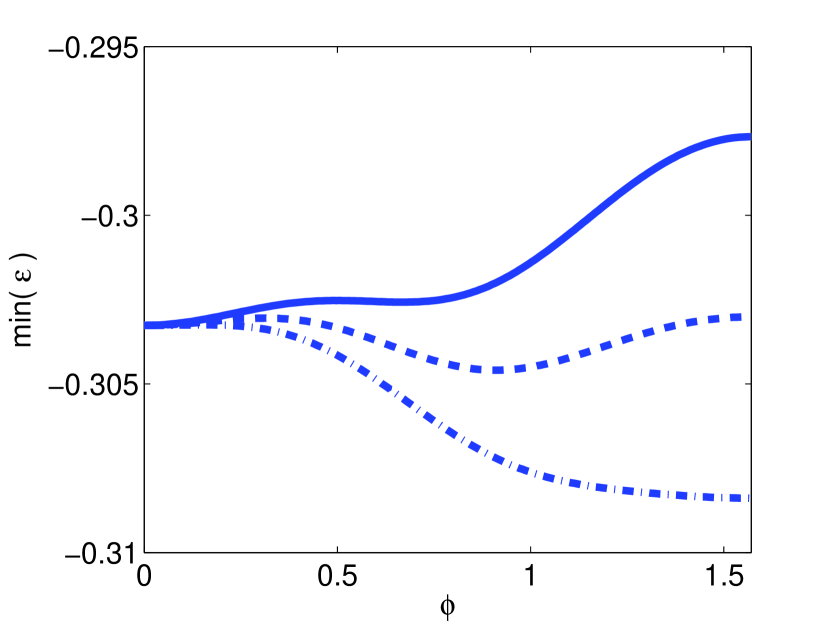
Figure 6: The plot shows the energy minimum versus the angle $\phi$ at $\eta=0.5$ and for different values of $\Gamma$: $\Gamma=0.234<\Gamma_{1}$ (solid line), $\Gamma\sim\Gamma_{fo}=0.237$ (dashed line) and $\Gamma=0.240>\Gamma_{2}$ (dot-dashed line).

This is illustrated in Fig. 6 where we plot the $\phi$-dependence of the minimal energy density for, respectively, $\Gamma=0.234<\Gamma_{1}$, $\Gamma=0.237$ (in the coexistence region) and $\Gamma=0.240>\Gamma_{2}$ (in both cases $\eta=0.5$). For $\Gamma<\Gamma_{1}$, the energy minimum is at $\phi=\pi/2$ (the EI state), while at $\Gamma>\Gamma_{2}$ the energy minimum is for $\phi=0$ (the SC state). Though the $\phi$-dependence of the minimal energy is, in general, rather complicated, the scale of the energy variations in all three cases is very small, i.e. the valley is practically flat. This is the reason for the narrow width of the disorder interval $\Gamma_{1}<\Gamma<\Gamma_{2}$, in which the two phases coexist - a very small variation of the disorder strength $\gamma$ is sufficient to shift the position the energy minimum from $\phi=\pi/2$ to $\phi=0$ along the energy valley, in which $\Delta=\sqrt{\Delta_{1}^{2}+\Delta_{2}^{2}}$ remains practically unchanged.

Figure 6 also illustrates the absence of first-order transitions in the model(1). Note that $\Gamma=0.237$ is close to $\Gamma_{\text{fo}}$, at which the energies of the SC and EI states become equal: $\langle f(0)\rangle=\langle f(\pi/2)\rangle$. The first-order transition between the two pure states, however, does not occur, since the energy has the global minimum at some angle $\phi$, such that $0<\phi<\pi/2$, corresponding to a mixed ground state. Furthermore, when $\Gamma=0.237$, the energy has a local maximum at $\phi=\pi/2$, enforcing the EI state to be metastable.

VI Discussion and Conclusions

We discussed effects of disorder in systems with competing instabilities, such as CDW superconductors. We considered a simple model, which describes a metal with two perfectly nested electron-like and hole-like parts of the Fermi surface. In this model the interplay between the electron-electron and electron-hole pairings is very strong, as these they compete over the whole Fermi surface.

We showed that disorder can be used to tune the balance between the two competing phases and to stabilize the state, in which they coexist. The charged nonmagnetic impurities induce superconductivity by suppressing the CDW state. Such a disorder-induced superconductivity is observed in the irradiated two-dimensional CDW material $2H$-TaS₂.mutka In other transition metal dichalcogenides, e.g. $2H$-NbSe₂ and $2H$-TaSe₂, which are CDW superconductors already in absence of disorder, a small amount of irradiation-induced defects results in an enhancement of $T_{c}$.mutka Similar behavior is observed in the quasi-one-dimensional CDW material Nb_1-xTa_xSe₃. In the pure NbSe₃, $T_{c}$ is smaller than $50$ mK at ambient pressure.Monceau The substitution of Nb for Ta suppresses the resistivity anomalies due to the CDW transitions, while $T_{c}$ grows up to $\sim 2$K at $x=0.05$.Fuller The effect of impurities in these materials is similar to that of pressure and hydrogen intercalation.Monceau ; Berthier ; Murthy

In agreement with these experimental findings, the phase diagrams of our model Figs. 3 and 4, show a strong sensitivity of the ground state to disorder and the coexistence of the SC and EI states in the presence of disorder. This behavior can be easily understood and described analytically, using the Landau expansion of the free energy in powers of the EI and SC order parameters near the quantum critical point [see Eq.(20)], which we derived from the microscopic model. Disorder distorts the shape of the energy potential and continuously shifts the position of the minimum from the point corresponding to the excitonic insulator to the point corresponding to the superconducting state, which gives rise to the coexistence of the two states.

The microscopic origin of this coexistence is the break-up of a part of the electron-hole pairs by disorder and the subsequent recombination of the released fermions into electron-electron and hole-hole pairs. In other words, disorder transforms the CDW gap in the single-electron density of states into a pseudogap, filled with states describing the broken electron-hole pairs. The SC phase develops inside this pseudogap, which resembles the behavior observed in high-T_c cuprates.Timusk

In addition to the disorder-induced superconductivity, resulting from the suppression of the EI state, the phase diagram of our model (see Fig. 3) shows an interesting ‘inverse’ effect, namely the suppression of the EI state due to the growth of the SC order parameter with decreasing temperature. Though this re-entrance transition is just another consequence of the competition between the two types of ordering, we did not find any reports of such a behavior in CDW superconductors in the literature. This, however, it has been observed in the quasi-one-dimensional spin-Peierls compound CuGeO₃, where impurities induce the long range Néel ordering.Kiryukhin In this material, the interplay between the dimerized and antiferromagnetic states allows for a similar theoretical description.MKK In most CDW superconductors the CDW transition occurs at a much higher temperature than the SC transition, so that the influence of the Cooper pairing on the CDW modulations is difficult to observe. Furthermore, the CDW gap only opens on a nested part of the Fermi surface. In quasi-one-dimensional NbSe₃ the fraction of the Fermi surface affected by the CDW transition was estimated to be $\sim 0.6$ at ambient pressure.Fuller In the two-dimensional $2H$-NbSe₂ this fraction is apparently very small, since the gap opening actually increases the conductivity of this materialharper and the part of the Fermi surface, where the gap opens, was not found in ARPES experiments,straub ; Valla ; Yokoya even though the gap value (34meV) is known.Wang For partially gapped Fermi surfaces the competition between the CDW and SC states is less strong, so that in $2H$-NbSe₂ they coexist even in absence of disorder.

While the enhancement of the SC transition temperature upon the suppression of the CDW state is well documented in many materials, the experimental situation with influence of the superconductivity on the CDW state is less clear. On the one hand, Raman experiments on $2H$-NbSe₂ show the suppression of the intensity the collective SC mode by magnetic field with the concomitant enhancement of the intensity of the CDW modes.Klein ; Peter On the other hand, no effect of the superconducting ordering below $7$K and of the suppression of the SC state by magnetic field on the CDW modulation was observed in x-ray experiments.Du The understanding of the behavior of $2H$-NbSe₂ is complicated by the multi-sheet structure of the Fermi surface and the momentum- and sheet-dependence of both order parameters. Yokoya The interplay between the CDW and SC states in this and other materials requires further experimental and theoretical studies.

Crucially, one may note that the phase diagram of the interacting system was inferred from the self-consistent Hartree-Fock approximation which captures only the mean-field characteristics. In view of the filamentary structure of the coexistence region, the system can be susceptible to mesoscopic or sample to sample fluctuations due to the quenched impurity potential. Such effects are recorded in fluctuations of the field $\Sigma(\mathbf{x})$ around its saddle-point or mean-field value (as opposed to the leading terms gathered in the low-order $\Gamma$ expansion considered here). In the gapless regime, such effects can give rise to long-ranged diffusion mode contributions to the generalized pair susceptibility (cf., e.g., Ref. [spivak_zhou, ]). However, in the present case, the disorder potential imposes a symmetry breaking perturbation on the EI phase. As such, we can expect mesoscopic fluctuations due to disorder to impose only a short-ranged (i.e. local on the scale of the coherence length of the EI order parameter) perturbation on the pair susceptibility. In the vicinity of the coexistence region, where the potential for the angle $\phi$ is shallow, the effect of these mesoscopic fluctuations may be significant.

To understand the effect of random fluctuations in the coexistence region, we consider the Ginzburg-Landau expansion for the ground state energy close to the quantum critical point $\eta=0,\Gamma=0$, at which the EI and SC states are degenerate. In the vicinity of this point the phase $\phi$ of the ‘total’ order parameter $\Delta_{1}+i\Delta_{2}=\Delta e^{i\phi}$ is a soft mode, so that weak disorder mainly induces spatial fluctuations of the phase, while the magnitude of the order parameter $\Delta$ approximately stays constant. As in the derivation of Eq.(21), we expand the energy in powers of $\Delta$ and disorder strength, assuming that $\Gamma\ll\Delta$, which is justified in the coexistence region, where $\Gamma\sim\frac{2\eta}{\pi}\Delta$ (see Eq.(16). Assuming that the phase varies slowly on the length scale of the correlation length $\xi=\frac{v_{F}}{\Delta}$, where $v_{F}$ is the Fermi velocity, we obtain

$$F\simeq\int d\mathbf{x}\left[\nu_{F}\left(\frac{v_{F}^{2}}{6}(\nabla\phi)^{2}+u(\mathbf{x})\cos 2\phi\right)+\langle f\rangle\right]\;,$$ (22)

where the first term describes the ‘elastic energy’ of an inhomogeneous state, the disorder-averaged free energy $\langle f\rangle$ is given by Eq.(21), and $u(\mathbf{x})$ is the fluctuating part of disorder coupled to the phase of the order parameter. Neglecting correlations on a scale smaller that the correlation length, $u(\mathbf{x})$ can be approximately considered as a random $\delta$-correlated Gaussian variable with zero average, $\langle u(\mathbf{x})\rangle=0$, and variance

$$\langle u({\bf x})u({\bf y})\rangle =A\delta({\bf x}-{\bf y}) A =\frac{\pi^{4}\Gamma^{2}\Delta^{2}}{2k_{F}^{3}}\;,$$ (23)

(we omit the lengthy calculations that lead to this result). The coupling to disorder also occurs in higher orders of the expansion, but those terms are relatively small and can be neglected.

Following the Imry and Ma argument,ImryMa we consider a large phase fluctuation, e.g., a droplet of the SC phase of the spatial extent $L$ inside the EI matrix. Comparing the typical energy gain due to the coupling to disorder $\sim\nu_{F}\sqrt{AL^{3}}$ with the loss in the elastic energy $\sim\nu_{F}v_{F}^{2}L$, we find that the fluctuation is energetically favorable for

$$L>\frac{v_{F}^{4}}{A}=\frac{v_{F}^{4}k_{F}^{3}}{2\pi^{2}\eta^{2}\Delta^{4}}\;,$$ (24)

where we took into account that, in the coexistence region, $\Gamma\sim\frac{2\eta}{\pi}\Delta$.

The crucial difference of our model from that considered in Ref.[ImryMa, ] is the absence of an exact continuous symmetry. Even in the coexistence region, the minimal-energy valley connecting the SC and EI points ($\phi=0$ and $\phi=\frac{\pi}{2}$) is not perfectly flat. The typical amplitude of the variations of the energy density is $\sim\eta^{2}\nu_{F}\Delta^{2}$ (see Eq. (21)), resulting in the energy loss $\sim\eta^{2}\nu_{F}\Delta^{2}L^{3}$ proportional the volume of the fluctuation, which suppresses large droplets. Comparing it with the energy gain, we find

$$L^{3}<\frac{A}{\eta^{4}\Delta^{4}}\;.$$ (25)

Equations (24) and (25) hold simultaneously for

$$v_{F}k_{F}<\eta\Delta\;,$$ (26)

which cannot be satisfied in the weak coupling limit. One may wonder why the condition (26) does not hold even for $\eta=\Gamma=0$, where the model has a continuous symmetry. The reason is that in our model the role of disorder is two-fold. On the one hand, it couples to the order parameter, as in the ‘random field’ model discussed in Ref.[ImryMa, ] and tends to destroy the ordering. On the other hand, it affects the energy difference between the EI and SC states and, therefore, suppresses the phase fluctuations, by destroying the symmetry of the energy potential. The second effect, which is linear in $\Gamma$, is stronger than the first.

Thus, the inhomogeneity of the order parameter, resulting from typical disorder fluctuations is small. The phase fluctuations can also be induced by large disorder fluctuations (’Lifshitz tails’), but their contribution to the free energy is exponentially small.Dotsenko This justifies our mean field treatment of disorder.

This conclusion may not hold, however, for strongly coupled CDW superconductors or for other types of disorder. Qualitatively, we expect that inhomogeneous excitonic and superconducting order parameters may result in a broadening of the coexistence region. The local suppression of the excitonic pairing near charged impurities can give rise to the local enhancement of the superconducting order. The state with such a nanoscale phase separation, in which two competing orders alternate in antiphase without a loss of the macroscopic coherence, can be more energetically favorable than the uniform state and, therefore, can be stabilized in a wider interval of parameters. Such a state was observed in $\mu$SR experiments on doped CuGeO₃, which shows both spin-Peierls and antiferromagnetic ordering.kojima

In conclusion, we studied effects of disorder on systems with competing superconducting and charge-density-wave instabilities. We showed that even in the extreme situation, when the competition takes place over the whole Fermi surface and the superconducting and charge-density-wave phases are mutually exclusive, disorder can give rise to their coexistence in a spatially homogeneous state. Furthermore, disorder itself can be used as a parameter, with which one can tune the balance between competing phases. Although our model is too simple to describe the physics behind the coexistence of superconductivity and CDW(SDW) states in, e.g., high-$T_{c}$ or heavy fermion materials, we believe that the ability of disorder to bring together incompatible phases may be important for understanding phase diagrams of these systems.

Appendix A Coexisting instabilities and derivation of the effective model

In this appendix we obtain a condition under which both the SC and EI instabilities can occur simultaneously. Here, we consider more realistic interactions between electrons than those described by the model (1), namely, the phonon-mediated interaction and the Coulomb repulsion. The Coulomb repulsion counteracts the phonon-mediated attraction between electrons and suppresses the SC instability. The same holds for the instability towards the formation of the excitonic condensate with the difference that the two types of interaction now change roles: the Coulomb force favors the electron-hole pairing, while the one-phonon exchange results in a repulsion between electrons and holes. We will show that the SC and EI instabilities can coexist due to different frequency dependence of the two types of interactions.

For retarded phonon-mediated interactions, the order parameters $\Delta_{1}$ and $\Delta_{2}$ are frequency-dependent, which complicates the solution of the self-consistency equations. We show, however, that in the weak coupling and weak disorder limit, the equations for the order parameters at zero frequency coincide with Eq. (9), which justifies the model introduced in Sec. II. Moreover, we will give the explicit expressions for the coupling constants $g_{1}$ and $g_{2}$ appearing in Eq. (1).

We describe effective electron-electron interactions by a non-local action

$$S_{\text{eff}}=\frac{g_{\text{e-ph}}^{2}}{2}\int d\mathbf{x}\int d\tau d\tau^{\prime}\rho(\mathbf{x},\tau)D(\tau-\tau^{\prime})\rho(\mathbf{x},\tau^{\prime})\\ +\frac{g_{C}^{2}}{2}\int d\mathbf{x}d\tau\rho^{2}(\mathbf{x},\tau)\;,$$ (27)

where $\rho=\sum_{\sigma}(\psi_{a\sigma}^{{\dagger}}\psi_{a\sigma}+\psi_{b\sigma}^{{\dagger}}\psi_{b\sigma})$ is the total electron density. The first term is the phonon-mediated effective attraction between electrons and $D(\tau-\tau^{\prime})$ is the phonon Green function. For a single dispersionless optical phonon with the frequency $\Omega_{0}$ and the propagator $D_{\omega_{n}}=-\Omega_{0}^{2}/(\omega_{n}^{2}+\Omega_{0}^{2})$, we have $D(\tau-\tau^{\prime})=-\Omega_{0}e^{-\Omega_{0}|\tau-\tau^{\prime}|}/2$ for $T\ll\Omega_{0}$. The second term in Eq. (27) is the instantaneous Coulomb interaction. We neglect the momentum dependence of the screened electron-phonon and Coulomb couplings, which makes the electron-electron interactions local in space.

The couplings for the $a$ and $b$-electrons in Eq.(27) give rise to a large freedom in the choice of order parameters, which in reality may not be present, e.g., due to the inter-band scattering, which separately does not conserve the numbers of the $a-$ and $b-$electrons. In what follows we restrict ourselves to the anomalous averages considered in Sec. II, which, for retarded interactions Eq. (27), are time-dependent ($j=a,b$ and $\sigma=\uparrow,\downarrow$):

$$\Delta_{1}(\tau-\tau^{\prime}) =-\left[g_{\text{e-ph}}^{2}D(\tau-\tau^{\prime})+g_{C}^{2}\right]\langle\psi_{i\uparrow}(\tau)\psi_{i\downarrow}(\tau^{\prime})\rangle$$

$$\Delta_{2}(\tau-\tau^{\prime}) =-\left[g_{\text{e-ph}}^{2}D(\tau-\tau^{\prime})+g_{C}^{2}\right]\langle\psi_{a\sigma}(\tau)\psi_{b\sigma}(\tau^{\prime})\rangle\;.$$

In the frequency representation the self-consistency equations read

$$\Delta_{1}(\omega_{n}) =-\frac{T}{4V}\sum_{\mathbf{p}\omega_{n}^{\prime}}\left(g_{\text{e-ph}}^{2}D_{\omega_{n}-\omega_{n}^{\prime}}-g_{C}^{2}\right)\rm{tr}\left(\tau_{1}G_{\mathbf{p},\omega_{n}^{\prime}}\right)$$

$$\Delta_{2}(\omega_{n}) =\frac{T}{4V}\sum_{\mathbf{p}\omega_{n}^{\prime}}\left(g_{\text{e-ph}}^{2}D_{\omega_{n}-\omega_{n}^{\prime}}-g_{C}^{2}\right)\rm{tr}\left(\tau_{3}\sigma_{1}G_{\mathbf{p},\omega_{n}^{\prime}}\right)\;,$$

where the electron Green function is given by Eq. (5).

To simplify the algebra, we consider here only the zero temperature case. The integration over the electron excitation energy $\xi$ gives

$$\begin{split}\Delta_{1}(\omega)=\frac{1}{2}\int_{-E_{c}}^{+E_{c}}d\omega^{\prime}\left[\kappa_{1}\frac{\Omega_{0}^{2}}{(\omega-\omega^{\prime})^{2}+\Omega_{0}^{2}}-\kappa_{2}\right]\frac{\tilde{\Delta}_{1}(\omega^{\prime})}{\sqrt{\tilde{\omega}^{\prime 2}+\tilde{\Delta}_{1}^{2}(\omega^{\prime})+\tilde{\Delta}_{2}^{2}(\omega^{\prime})}}\\ \Delta_{1}(\omega)=\frac{1}{2}\int_{-E_{c}}^{+E_{c}}d\omega^{\prime}\left[\kappa_{2}-\kappa_{1}\frac{\Omega_{0}^{2}}{(\omega-\omega^{\prime})^{2}+\Omega_{0}^{2}}\right]\frac{\tilde{\Delta}_{1}(\omega^{\prime})}{\sqrt{\tilde{\omega}^{\prime 2}+\tilde{\Delta}_{1}^{2}(\omega^{\prime})+\tilde{\Delta}_{2}^{2}(\omega^{\prime})}}\end{split}$$ (28)

where we have introduced the dimensionless coupling constants, $\kappa_{1}=\nu_{F}g_{\text{e-ph}}^{2}$ and $\kappa_{2}=\nu_{F}g_{C}^{2}$, and where $E_{c}$ is the frequency cutoff required for the instantaneous Coulomb interaction. Moreover the variables $\tilde{\omega},\tilde{\Delta}_{1},$ and $\tilde{\Delta}_{2}$ are defined in (6).

Although Eqs. (28) look at a first sight complicated, one can see that, in the limit of weak coupling and weak disorder, $\Delta_{1,2},\Gamma\ll\Omega_{0}<E_{c}$, their solution can be found by making use of the fact that the order parameters $\Delta_{1}(\omega)$ and $\Delta_{2}(\omega)$ strongly vary at frequencies $\omega\sim\Omega_{0}$, while $\tilde{\omega}$, $\tilde{\Delta}_{1}$, and $\tilde{\Delta}_{2}$ are nontrivial functions of $\omega$ only at much lower frequencies $\omega\sim\Gamma$, where $\Delta_{1}(\omega)$ and $\Delta_{2}(\omega)$ can be replaced by their zero frequency values. Therefore, we can solve Eqs. (28) in two steps: first we find the frequency dependence of the order parameters $\Delta_{1}(\omega)$ and $\Delta_{2}(\omega)$ for arbitrary values of $\Delta_{1}(0)$ and $\Delta_{2}(0)$, and then we solve the self-consistency equations for $\Delta_{1}(0)$ and $\Delta_{2}(0)$.

It is convenient to use the dimensionless variables $x=\omega/\Omega_{0}$ and $y_{1,2}(x)=\Delta_{1,2}(\omega)/\Omega_{0}$ (and similarly $\tilde{x}$ and $\tilde{y}_{1,2}(x)$), in terms of which the first of the equations (28) reads

$$y_{1}(x)=\int_{0}^{\Lambda}dx^{\prime}\frac{\tilde{y}_{1}(x^{\prime})}{\sqrt{\tilde{x}^{\prime 2}+\tilde{y}_{1}^{2}(x^{\prime})+\tilde{y}_{2}^{2}(x^{\prime})}}\\ \left\{\frac{\kappa_{1}}{2}\left[\frac{1}{(x+x^{\prime})^{2}+1}+\frac{1}{(x-x^{\prime})^{2}+1}\right]-\kappa_{2}\right\}\;,$$

where $\Lambda=E_{c}/\Omega_{0}$. We then introduce an intermediate scale $X$, such that $y_{1,2}\ll X\ll 1$. In the interval $0\leq x^{\prime}\leq X$, we can neglect the $x^{\prime}$-dependence of the kernel of this integral equation and the functions $y_{1,2}(x^{\prime})$ (however, $\tilde{y}_{1,2}$ and $\tilde{x}^{\prime}$ still do depend on $x^{\prime}$). In the second interval $X\leq x^{\prime}\leq\Lambda$, we substitute $\tilde{y}_{1}/\sqrt{\tilde{x}^{\prime 2}+\tilde{y}_{1}^{2}+\tilde{y}_{2}^{2}}$ by $y_{1}(x^{\prime})/x^{\prime}$ and perform the integration by parts. In this way we obtain

$$y_{1}(x)=-y_{1}(\Lambda)\kappa_{2}\ln\Lambda+\left(\frac{\kappa_{1}}{1+x^{2}}-\kappa_{2}\right)\left[\int_{0}^{X}dx^{\prime}\frac{\tilde{y}_{1}(x^{\prime})}{\sqrt{\tilde{x}^{\prime 2}+\tilde{y}_{1}^{2}(x^{\prime})+\tilde{y}_{2}^{2}(x^{\prime})}}-y_{1}(0)\ln X\right]\\ -\int_{0}^{\infty}dx^{\prime}\ln x^{\prime}\frac{d}{dx^{\prime}}\left\{\left[\frac{\kappa_{1}}{2}\left(\frac{1}{(x+x^{\prime})^{2}+1}+\frac{1}{(x-x^{\prime})^{2}+1}\right)-\kappa_{2}\right]y_{1}(x^{\prime})\right\}\;,$$ (29)

where the limits of the second integration were extended to $0$ and $\infty$, as there is convergence both at small and large frequencies.

Since, at $X\gg y_{1,2}$, Eq. (29) is independent of $X$, we can chose $X=1$ (and still substitute $y_{1,2}(x^{\prime})$ by $y_{1,2}(0)$ in the first integral). The value of $y_{1}$ at the cutoff is then given by

$$y_{1}(\Lambda)=-\kappa_{2}^{*}\left[\int_{0}^{1}dx^{\prime}\frac{\tilde{y}_{1}(x^{\prime})}{\sqrt{\tilde{x}^{\prime 2}+\tilde{y}_{1}^{2}(x^{\prime})+\tilde{y}_{2}^{2}(x^{\prime})}}\right.\\ \left.-\int_{0}^{\infty}dx\ln x\frac{dy_{1}}{dx}\right]\;,$$

where $\kappa_{2}^{\ast}=\kappa_{2}/(1+\kappa_{2}\ln\Lambda)$. For arbitrary $x$ we have

$$y_{1}(x)=\left(\frac{\kappa_{1}}{1+x^{2}}-\kappa_{2}^{\ast}\right)I(y_{1}(0),y_{2}(0))\\ -\int_{0}^{\infty}dx^{\prime}\ln x^{\prime}\frac{d}{dx^{\prime}}\left\{\left[\frac{\kappa_{1}}{2}\left(\frac{1}{(x+x^{\prime})^{2}+1}\right.\right.\right.\\ \left.\left.\left.+\frac{1}{(x-x^{\prime})^{2}+1}\right)-\kappa_{2}^{\ast}\right]y_{1}(x^{\prime})\right\}\;,$$ (30)

where the notation

$$I(y_{1}(0),y_{2}(0))=\int_{0}^{1}dx^{\prime}\frac{\tilde{y}_{1}(x^{\prime})}{\sqrt{\tilde{x}^{\prime 2}+\tilde{y}_{1}^{2}(x^{\prime})+\tilde{y}_{2}^{2}(x^{\prime})}}$$

is used to stress the fact that $y_{1}$ and $y_{2}$ are assumed to be frequency independent.

In the weak coupling limit the first term in the right-hand side of Eq. (30), proportional to the ‘large logarithm’ $\ln\sqrt{y_{1}^{2}+y_{2}^{2}}$, is much larger than the second term, so this integral equation can be solved by iterations, which generate a perturbative expansion for $y_{1}(x)$. To the lowest order, the frequency dependence of the order parameter coincides with that of the kernel:AndersonMorel

$$y_{1}(x)=\left(\frac{\kappa_{1}}{1+x^{2}}-\kappa_{2}^{\ast}\right)I(y_{1}(0),y_{2}(0))\;.$$ (31)

Then the self-consistency equation for $\Delta_{1}(0)$ coincides with Eq. (9) at $T=0$:

$$\Delta_{1}(0)=\lambda_{1}\int_{0}^{\Omega_{0}}d\omega\frac{\tilde{\Delta}_{1}(\omega)}{\sqrt{\tilde{\omega}^{2}+\tilde{\Delta}_{1}^{2}(\omega)+\tilde{\Delta}_{2}^{2}(\omega)}}\;,$$ (32)

and the effective coupling constant is given by

$$\lambda_{1}=\kappa_{1}-\kappa_{2}^{\ast}=\kappa_{1}-\frac{\kappa_{2}}{1+\kappa_{2}\ln E_{c}/\Omega_{0}}\;.$$ (33)

The negative term in the coupling constant describes the reduction of the attraction between electrons due to the Coulomb repulsion, but this reduction is itself reduced by the presence of the large logarithm in the denominator due to the difference in the time scales of the retarded phonon-mediated attraction and the Coulomb repulsion.Bogoliubov ; AndersonMorel The first-order correction to $y_{1}(x)$, found by substituting Eq. (31) into the integral in Eq. (30) (as well as all higher-order corrections), leaves the form of the self-consistency equation (32) unchanged, but results in a small modification of the expression for the effective coupling constant through $\kappa_{1}$ and $\kappa_{2}$:

$$\lambda_{1}=\kappa_{1}\left(1-\frac{\kappa_{1}}{2}\right)-\kappa_{2}^{\ast}\;.$$

The frequency dependence of the excitonic insulator order parameter $\Delta_{2}(\omega)$ and the self-consistency equation for $\Delta_{2}(0)$ can be obtained from Eqs.(32,33) by the substitution $\Delta_{1}\mapsto\Delta_{2}$, $\kappa_{1}\mapsto-\kappa_{1}$, and $\kappa_{2}\mapsto-\kappa_{2}$:

$$\Delta_{2}(0)=\lambda_{2}\int_{0}^{\Omega_{0}}d\omega\frac{\tilde{\Delta}_{2}(\omega)}{\sqrt{\tilde{\omega}^{2}+\tilde{\Delta}_{1}^{2}(\omega)+\tilde{\Delta}_{2}^{2}(\omega)}}\;,$$ (34)

where the effective coupling constant $\lambda_{2}$ is to the lowest order given by

$$\lambda_{2}=\frac{\kappa_{2}}{1-\kappa_{2}\ln E_{c}/\Omega_{0}}-\kappa_{1}\;.$$ (35)

In Fig. 2 we show the typical frequency dependence of the SC and EI order parameters, calculated for $\kappa_{1}=0.25$ and $\kappa_{2}=0.1$ and $\Gamma=0$. (Since in the absence of disorder the SC and EI states cannot coexist, we calculated $\Delta_{1}(\omega)$ assuming $\Delta_{2}=0$ and vice versa.) The SC order parameter $\Delta_{1}(\omega)$ is positive at small frequencies and changes sign at $\omega\simeq\Omega_{0}$, while the EI order parameter $\Delta_{2}(\omega)$ has a dip for $|\omega|<\Omega_{0}$. The ‘separation’ of the two order parameters in frequency is crucial for the coexistence of instabilities.

The necessary condition for superconductivity to appear is $\lambda_{1}>0$, while the instability towards the excitonic condensate occurs for $\lambda_{2}>0$. These two conditions,

$$\lambda_{1} >\frac{\lambda_{2}}{1+\lambda_{2}\ln\Lambda} \lambda_{1} <\frac{\lambda_{2}}{1-\lambda_{2}\ln\Lambda}\;,$$

hold simultaneously for

$$|\eta|=\left|\frac{1}{\lambda_{1}}-\frac{1}{\lambda_{2}}\right|<\ln\frac{E_{c}}{\Omega_{0}}\;.$$ (36)

A weak disorder has little effect on the frequency dependence of $\Delta_{1}$ and $\Delta_{2}$. However, its presence is crucial for the stabilization of the mixed state, in which the two order parameters coexist.

- (1) For a recent review see, e.g., A.M. Gabovich, A.I. Voitenko, and M. Ausloos, Phys. Rep. 367, 583 (2002).
- (2) A.M. Gabovich, A.I. Voitenko, J.F. Annett, and M. Ausloos, Supercond. Sci. Technol. 14 R1 (2001).
- (3) J.A. Wilson, F.D. DiSalvo, S. Mahajan, Adv. Phys. 24, 117 (1975).
- (4) D. Jérome, C. Berthier, P. Moliné, J. Rouxel, J. Physique Colloc. 437, C125 (1976).
- (5) C. Berthier, P. Molinié, and D. Jérome, Solid State Commun. 18, 1393 (1976).
- (6) W.W. Fuller, P.M. Chaikin, and N.P. Ong, Phys. Rev. B 24, 1333 (1981).
- (7) R.K. Stanley, R.C. Morris, and W.G. Moulton, Phys. Rev. B 20 1903 (1979).
- (8) L.H. Cadwell, R.C. Morris, and W.G. Moulton, Phys. Rev. B 23, 2219 (1981).
- (9) H. Mori, I. Hirabayashi, S. TanakaTakehiko Mori, Y. Maruyama, and H. Inokuchi, Solid State Commun. 80, 411 (1991).
- (10) J. Merino and R. H. McKenzie, Phys. Rev. Lett. 87, 237002 (2001).
- (11) D.E. Moncton, J.D. Axe, and F.J. DiSalvo, Phys. Rev. Lett. 34, 734 (1975).
- (12) J.M.E. Harper, T.H. Geballe, and F.J. DiSalvo, Phys. Lett. 54A, 27 (1975).
- (13) Th. Straub, Th. Finteis, R. Claessen, P. Steiner, S. Hüfner, P. Blaha, C.S. Oglesby, and E. Bucher, Phys. Rev. Lett. 82, 4504 (1999).
- (14) T. Valla et al., Phys. Rev. Lett. 92, 086401 (2004).
- (15) C.H-Du et al., J. Phys.: Condens. Matter 12, 5361 (2000).
- (16) P. Monceau, J. Peyrard, J. Richard, and P. Molinie, Phys. Rev. Lett. 39, 161 (1976).
- (17) D.W. Murphy, F.J. DiSalvo, G.W. Hull, Jr., J.V. Wasczak, S.F. Meyer, G.R. Stewart, S. Early, J.V. Acrivos, and T.H. Geballe. J. Chem. Phys. 62, 967 (1975).
- (18) P. W. Anderson, J. Phys. Chem. Sol. 11, 26 (1959).
- (19) H. Mutka, Phys. Rev. B 28, 2855 (1983); H. Mutka, N. Housseau, J. Pelissier, R. Ayroles, and C. Roucau, Solid State Commun. 50, 161 (1984).
- (20) G.S. Grest, K. Levin, and M.J. Nass, Phys. Rev. B 25, 4562 (1982).
- (21) L. V. Keldysh and Yu. V. Kopaev, Fiz. Tverd. Tela (Leningrad) 6, 2791 (1964) [Sov. Phys. Solid State 6, 2219 (1965)]; L. V. Keldysh and A. N. Kozlov, Zh. Éksp. Teor. Fiz. 54, 978 (1968) [Sov. Phys. JETP 27, 521 (1968)].
- (22) A.I. Rusinov, D.C. Kat, and Yu.V. Kopaev, Zh. Eksp. Teor. Fiz. 65, 1984 (1973) [Sov. Phys. JETP 38, 991 (1974)].
- (23) J. Zittartz, Phys. Rev. 164, 575 (1967).
- (24) A.A. Abrikosov and L.P. Gor’kov, Zh. Eksp. Teor. Fiz. 39, 1781 (1960) [Sov. Phys. JETP 12, 1243 (1961)].
- (25) P. Morel and P.W. Anderson, Phys. Rev. 125, 1263 (1962).
- (26) S. F. Edwards and P. W. Anderson, J. Phys. F 5, 965 (1975).
- (27) M. Mostovoy, D. Khomskii, and J. Knoester, Phys. Rev. B 58, 8190 (1998).
- (28) V. Kiryukhin, Y. J. Wang, S. C. LaMarra, R. J. Birgeneau, T. Masuda, I. Tsukada, and K. Uchinokura, Phys. Rev. B 61, 9527 (2000).
- (29) A.I. Solomon and J.L. Birman, J. Math. Phys. 28, 1526 (1987).
- (30) S.C. Zhang, Science 275, 1089 (1997).
- (31) Y. Kitaoka, K. Ishida, Y. Kawasaki, O. Trovarelli, C. Geibel and F. Steglich, J. Phys. Condens. Matter 13, L79 (2001).
- (32) T. Timusk and B. Slatt, Rep. Prog. Phys. 62, 61 (1999).
- (33) T. Yokoya et al., Science 294, 2518 (2001).
- (34) C. Wang, B. Giambattista, C.G. Slough, R. V. Coleman, and M. A. Subramanian, Phys. Rev. B 42, 8890 (1990).
- (35) R. Sooryakumar and M.V. Klein, Phys. Rev. Lett. 45, 660 (1980); Phys Rev. B 23 3213 (1981); R. Sooryakumar, M.V. Klein, and R.F. Frindt, Phys. Rev. B 23 3222 (1981).
- (36) P.B. Littlewood and C.M. Varma, Phys. Rev. Lett. 47, 811 (1981); Phys. Rev. B 26, 4883 (1982).
- (37) B. Spivak and F. Zhou, Phys. Rev. Lett. 74, 2800 (1995).
- (38) Y.Imry and S.-K. Ma, Phys. Rev. Lett. 35, 1399 (1975).
- (39) V. Dotsenko, J. Phys. A: Math. Gen. 27, 3397 (1994).
- (40) K.M. Kojima, Y. Fudamoto, M. Larkin, G.M. Luke, J. Merrin, B. Nachumi, Y.J. Uemura, M. Hase, Y. Sasago, K. Uchinokura, Y. Ajiro, A. Revcolevschi, and J.-P. Renard, Phys. Rev. Lett. 79, 503 (1997).
- (41) N.N. Bogoliubov, V.V.Tolmachev, and D.V. Shirkov, “A new method in the theory of superconductivity” (Consultants bureau, New York, 1959).