Spin Splitting and Spin Current in Strained Bulk Semiconductors

Abstract

We present a theory for two recent experiments in bulk strained semiconductors kato1 ; kato2 and show that a new, previously overlooked, strain spin-orbit coupling term may play a fundamental role. We propose simple experiments that could clarify the origin of strain-induced spin-orbit coupling terms in inversion asymmetric semiconductors. We predict that a uniform magnetization parallel to the electric field will be induced in the samples studied in kato1 ; kato2 for specific directions of the applied electric field. We also propose special geometries to detect spin currents in strained semiconductors.

Spin manipulation in semiconductors has seen remarkable theoretical and experimental interest in recent years with the advent of spin-electronics and with the realization that strong spin-orbit coupling in certain materials can influence the transport of carriers in so-called spintronics devices wolf . In particular, the issue of creating spin polarization of carriers in nonmagnetic semiconductors with spin-orbit coupling using only electric fields has caused a flurry of theoretical and experimental activity murakami1 ; sinova ; Dyakonov:1971 ; Hirsch:1999 ; Zhang:2000 ; Levitov:1985 ; Edelstein:1990 ; Aronov:1991 ; Magarill:2001 ; Chaplik:2002 ; Inoue:2003 ; Cartoixa:2001 ; Silsbee:2001 . Two kinds of theories of spin-polarization under the action of an electric field have been put forward. The first kind, dating back since the mid 1980’s Levitov:1985 , predicts the existence of a spatially homogeneous net spin polarization perpendicular to the applied electric current in two dimensional samples with spin-orbit interaction. This effect is dissipative and has been recently observed experimentally ganichev . There also exist two very recent murakami1 ; sinova theories predicting non-dissipative, intrinsic spin currents with the spin polarization and flow direction perpendicular to each other and to the electric field. This effect does not create a bulk magnetization but, if observed, can be used for spin injection, and its validity is being experimentally tested at the present time. One of the theories sinova predicts a spin current polarized out of plane and flowing perpendicular to the in-plane electric field applied on a $2$-dimensional semiconductor sample exhibiting Rashba spin-orbit coupling. As long as the Rashba spin splitting is large enough, the spin conductivity is ’universal’ ($e/8\pi\hbar$) in the sense that it does not depend on the value of the coupling. The other effect murakami1 appears in the valence band of the bulk samples and is proportional to the spin-orbit splitting of the valence bands (to the difference between the Fermi momenta of the heavy and light-hole bands).

In the first part of this letter we analyze the theory behind two recent experiments in bulk strained semiconductors kato1 ; kato2 where an electric-field-induced uniform homogeneous spin polarization upon an applied electric field is observed. We make the case that the observed spin-splitting (whose origin is puzzling) and spin polarization is due to a previously overlooked strain-spin-splitting term, and propose easy experimental checks of our theory.

In the second part of this letter we predict the appearance of an intrinsic spin polarized spin current in n-doped bulk (and 2 dimensional) strained semiconductors (GaAs, GaSb, InSb, InGaAs, AlGaAS, etc) under the influence of an electric field. The spin conductance is ’universal’, in the sense that it does not depend on the value of strain (for large enough strain), but it is proportional to the average Fermi momentum of the conduction band. The effect is due to the spin-orbit splitting of the conduction band under strain and is hence absent in strain-free semiconductors. The very long spin relaxation time in the conduction band as well as the relative penetration of strain engineering in semiconductor industry applications make this effect of potential technological importance. We propose an experimental technique using the already existing setup in kato1 ; kato2 to measure the spin current and to differentiate between the intrinsic spin current and the uniform magnetization effects.

In kato1 nine samples of n-doped ($n=3\times 10^{16}cm^{-3}$) $In_{x}Ga_{1-x}As$ ($x=5\%-7\%$) of thicknesses between $200nm-1500nm$, grown in the $[001]$ direction on undoped GaAs substrate, are used to probe the electron spin dynamics through time and spatially resolved Faraday rotation (FR). The length and width of the samples are roughly $300\mu m\times 80\mu m$. The lattice mismatch provides for diagonal strain in the $x,y,z=[100],[010],[001]$ directions of $0.04\%-0.46\%$ kato3 (contrary to claims in culcer , the lattice constants in $x$ and $y$ directions are also strained, this being a generic feature of $[001]$ growth). Moreover, anisotropic shear strain develops in all directions ($xy,xz,yz=[110],[101],[011]$) due to different direction-dependent strain relaxation rates at the growth temperature of around $500C$ kavanagh . This guarantees that all the components of the strain tensor $\epsilon_{ij},\;i,j=x,y,z$ are non-zero and of the same order of magnitude. The magnitude of the strain components is given in Table[1].

Pump-probe FR beams measure the total magnetization of the optically injected electron spins in the growth direction $z$ when the samples are placed in an electric field on the $[110]$ and $[1\bar{1}0]$ directions, respectively. The dynamics of the spin packet is mainly described by a precession around a total magnetic field $\vec{B}_{tot}=\vec{B}_{int}+\vec{B}_{ext}$ where $\vec{B}_{ext}$ is an externally applied magnetic field whereas $\vec{B}_{int}$ is the momentum-dependent internal magnetic field caused by the spin-orbit coupling. The precession around a $\vec{B}_{int}$ is the main feature of most of the spintronics devices, starting with the Das-Datta spin-field transistor dasdatta . Under an applied electric field, the average particle momentum acquires a non-zero value, parallel to the electric field. The internal magnetic field is caused by the spin orbit coupling: the electric field acts on the particle momentum which in turn couples to the spin. The signal at the probe beam can be fitted to $\cos(g\mu_{B}|\vec{B}_{int}+\vec{B}_{ext}|\Delta t/\hbar)$ where $\mu_{B}$ is the Bohr magneton, $g$ is the electron $g$-factor while $\Delta t$ is the temporal delay between the pump and probe pulses. This fit gives the direction and value of $\vec{B}_{int}$ which turns out to be perpendicular to the applied electric field $E$ and the $\hat{z}$ axis (for $E$ in-plane); the value of $\vec{B}_{int}$ is used to determine the spin splitting $\Delta_{0}=g\mu_{B}B_{int}$ and a phenomenological relation $\Delta_{0}=\beta v_{d}$ is observed where $v_{d}$ is the spin-drift velocity and $\beta$ is a constant of proportionality that is the focus of the experiment kato1 . Experiments find that $v_{d}$ is linearly proportional to the electric field $E$.

As a first step, let us theoretically address the question of origin of $\beta$. By group theory, inversion symmetry breaking bulk strained semiconductors exhibit three main types of spin splitting pikustitkov :

$$H=\frac{\hbar^{2}}{2m}k^{2}+H_{1}+H_{2}+H_{3},\\ H_{1}=\lambda[\sigma_{x}k_{x}(k_{y}^{2}-k_{z}^{2})+\sigma_{y}k_{y}(k_{z}^{2}-k_{x}^{2})+\sigma_{z}k_{z}(k_{x}^{2}-k_{y}^{2})]\\ H_{2}=\frac{1}{2}C_{3}[\sigma_{x}(\epsilon_{xy}k_{y}-\epsilon_{xz}k_{z})+\sigma_{y}(\epsilon_{yz}k_{z}-\epsilon_{yx}k_{x})+\\ +\sigma_{z}(\epsilon_{zx}k_{x}-\epsilon_{zy}k_{y})]\\ H_{3}=D[\sigma_{x}k_{x}(\epsilon_{zz}-\epsilon_{yy})+\sigma_{y}k_{y}(\epsilon_{xx}-\epsilon_{zz})+\sigma_{z}k_{z}(\epsilon_{yy}-\epsilon_{xx})]$$ (1)

$m=0.0665m_{0}$ is the effective electron mass in the conduction band vurgaftman , $\lambda,C_{3},D>0$ are material constants, $\sigma_{x,y,z}$ are the 3 spin-Pauli matrices,and $\epsilon_{ij},\;\;i,j=x,y,z$ are the components of the symmetric strain tensor.

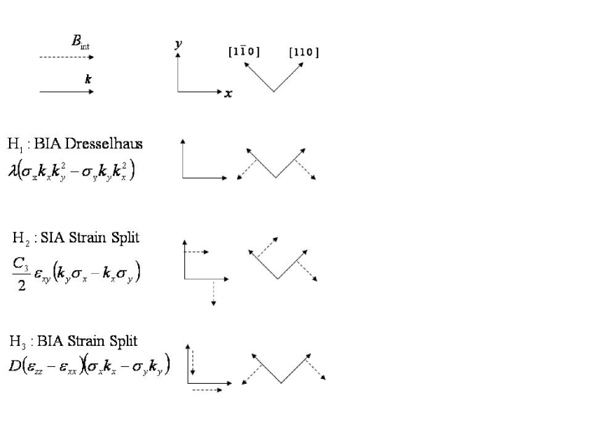
Figure 1: Direction of the internal magnetic field $\vec{B}_{int}$ for the three spin splitting Hamiltonians $H_{1},H_{2},H_{3}$, ($\lambda,C_{3},D>0$) considering the electric field $E$ (and hence the average momentum) to be in plane. It was also assumed that $\epsilon_{xx}=\epsilon_{yy}$, as appropriate in the experiment kato1 . The experimental SIA data cannot be explained by the term $H_{2}$, but nevertheless, the SIA-type $B_{int}$ seen in the experiment has the same direction as the one plotted here. When $E||x$ or $E||y$, the BIA term $H_{3}$ induces a $B_{int}||E$ whereas the BIA term $H_{1}$ does not induce spin splitting for these directions. This constitutes a simple check of the experiment

All three Hamiltonians can be written as the coupling of a fictitious $k$-dependent internal magnetic field $\vec{B}_{int}$ to the electron spin, $\vec{B}_{int}(k)\vec{\sigma}=B_{x}(k)\sigma_{x}+B_{y}(k)\sigma_{y}+B_{z}(k)\sigma_{z}$ (an overall factor of $g\mu_{B}$ has been absorbed into the definition of $B$ to simplify notation). The directions of $\vec{B}_{int}$ as dependent on the directions of $\vec{k}$ are shown in Fig[1]. The SIA-type term gives a $\vec{B}_{int}$ that keeps its orientation as $\vec{k}$($||\vec{E}$) is rotated between the $[110]$ and $[1\bar{1}0]$ directions, while both BIA-type $\vec{B}_{int}$ coming from $H_{1}$ and $H_{3}$ change their sign between $[110]$ and $[1\bar{1}0]$. The difference between $H_{1}$ and $H_{3}$ is that the latter has a finite $\vec{B}_{int}$ when $\vec{E}||x,y$ whereas the former has zero $B_{int}$ for the same directions.

In kato1 the values of the splitting $\beta$ are measured on the $[110]$ and $[1\bar{1}0]$ directions and because of the sign-changing properties of $\vec{B}_{int}$ mentioned above, the BIA and the SIA contributions to $\beta$ can be obtained as follows: $\beta_{BIA}=(\beta_{[110]}-\beta_{[1\bar{1}0]})/2,\;\beta_{SIA}=(\beta_{[110]}+\beta_{[1\bar{1}0]})/2$. Surprisingly, the spin splitting is more of a BIA-type rather than an SIA-type, contradicting the conventional knowledge that an SIA-type term described by $H_{2}$ is responsible for spin splitting in strained semiconductors pikustitkov ; hassenkam ; howlett ; khaetskii ; bahder ; seiler .

Theoretically, the Dresselhaus term $H_{1}$ is a bulk-inversion asymmetry term that appears even in the absence of strain. As observed in the experiment, the fictitious internal magnetic field $\vec{B}_{int}$ is perpendicular to the momentum $\vec{k}$: $\vec{B}_{int}(k)\vec{k}=0$, where $B_{x}=\lambda k_{x}(k_{y}^{2}-k_{z}^{2})$, $B_{y}$ and $B_{z}$ being obtained by cubic permutation. For GaAs, the constant $\lambda=22eV\AA^{3}$. However, we believe this term is not responsible for the spin splitting observed in the experiment kato1 . The observed splitting is linear in momentum $k$, inconsistent with the $H_{1}\sim k^{3}$. Experiments performed on InSb seiler , another material with inversion asymmetry, support this conclusion and point strongly to the fact that strained InSb is described by $H_{2}$. In seiler stress of up to $4$ kbar is applied mechanically on a $1\times 1\times 10mm^{3}$ sample and Shubnikov-de-Haas oscilations are used to probe the band structure. Without applied strain, the conduction band exhibits a spin-splitting that is small and cubic in $k$, described by $H_{1}$. In seiler the application of diagonal does not induce any observable spin splitting whereas the application of shear strain induces a splitting linear in $k$, described by $H_{2}$. Relatively large stress-induced splitting of the Fermi surfaces occurs in the lower concentration ($n=1.4\times 10^{15}-2.0\times 10^{17}cm^{-3}$) samples seiler . The energy splitting dispersion switches from $k^{3}$ in the unstrained case to $k$ when strain (stress) above $1kbar$ is applied, in accordance to $H_{2}$ becoming dominant over $H_{1}$. From a theoretical estimate, at $n=3\times 10^{16}cm^{-3}$, $H_{1}$ should be of the same size as $H_{3}$ and roughly one order of magnitude lower than $H_{2}$. The spin splitting at the Fermi wavevector $k_{F}=0.96\times 10^{8}m^{-1}$ due to $H_{1}$ is less than $10^{-5}eV$. By contrast the spin splitting due to $H_{2}$ is $C_{3}\epsilon_{xy}k_{F}=5.06\times 10^{-2}\epsilon_{xy}eV=5\times 10^{-5}-15\times 10^{-5}eV$ for $\epsilon_{xy}=0.1\%-0.3\%$ as in kato1 (see Table[1] for conversion of strain components from kato1 to the orthogonal system $\epsilon_{xy}$). An experimental value of $C_{3}/\hbar=8\times 10^{5}m/s$ for GaAs was used d'yakonov . Contrary to previous remarks culcer , there is hence no theoretical or experimental a-priori reason to disregard the strain-dependent spin splitting terms in favor of the Dresselhaus $k^{3}$ term for the doping values in the experiment kato1 .

There are a number of experimental reasons in kato1 hinting the marginal significance of the $k^{3}$ term. In kato1 strain plays a critical role in generating the spin-orbit coupling $\vec{B}_{int}$. Samples prepared from the same wafer but unstrained show a reduction by an order of magnitude of $B_{int}$ along both the $[110]$ and the $[1\bar{1}0]$ directions. If $H_{1}$ were responsible for spin splitting, its value would remain unchanged upon varying strain. Strain could only enter the system through the variation of the effective electron mass in the $x,y,z$ directions, as culcer points out. However, these variations with strain are of a maximum $2\%-3\%$ culcer ; vurgaftman thereby not accounting for the order of magnitude variation of the spin-splitting between the strained and the unstrained cases observed in kato1 .

The term $H_{2}$ is a structural inversion asymmetry (SIA)-type term that has its origin in the acoustic phonon interaction of the valence band with the conduction band pikustitkov . In the framework of the Kane’s $8\times 8$ matrix ($2\times 2$ for the conduction and split-off band and $4\times 4$ for the valence band) the conduction band couples to the valence band. In systems with inversion symmetry where the selection rules for L are satisfied, it is impossible to couple spin-$0$ ($|s\rangle$) with spin-$1$ ($|z\rangle$) through a spin-$2$ term ($\epsilon_{ij}$) and hence $\langle s|\epsilon_{xy}|z\rangle=0$. However, when inversion symmetry is broken, the fore-mentioned term need not be zero as the L selection rule need not apply. Upon straining, the matrix elements between the conduction and valence band have the form $\langle s|\epsilon_{xy}|z\rangle$ (plus cyclic permutations) where $|s\rangle$ is the $s$-orbital and $|z\rangle$ is one of the $p$ orbitals. Through perturbation theory, one can compute the effect of this valence-conduction band interaction when projected to the conduction band and obtain the conduction band effective Hamiltonian $H_{2}$ pikustitkov ; howlett ; khaetskii ; bahder . Taking into account that the electric field is in-plane ($<k_{z}>=0$) and that $\epsilon_{xy}\neq 0$ (see Table[1]), in $H_{2}$ the components of the internal magnetic field (which due to the rescaling by $g\mu_{B}$ has units of energy) are: $B_{x}=\frac{1}{2}C_{3}\epsilon_{xy}k_{y},\;B_{y}=-\frac{1}{2}C_{3}\epsilon_{yx}k_{x}=-\frac{1}{2}C_{3}\epsilon_{xy}k_{x}$. Switching coordinates to the $[110]$ and $[1\bar{1}0]$ directions, $B_{[110]}=\frac{1}{2}C_{3}\epsilon_{xy}k_{[1\bar{1}0]},\;B_{[1\bar{1}0]}=-\frac{1}{2}C_{3}\epsilon_{xy}k_{[110]}$ (see Fig[1]. Since $H_{2}$ is an SIA term, the spin splitting $\beta$ will be of SIA type $\beta^{th}_{SIA}$ (th stands for the theoretical estimate). Since $<k>=\frac{1}{\hbar}mv_{d}$ where $v_{d}$ is the drift velocity of the spin packed due to the electric field, we get a simple formula for the

$$\beta^{th}_{SIA}=\frac{C_{3}}{\hbar}\epsilon_{xy}m$$ (2)

By using the experimentally known value for $C_{3}/\hbar=8\times 10^{5}m/2$, the predicted values for $\beta^{th}_{SIA}$ are given in Table 1. The theoretical values are larger than the observed ones by a factor of $3-30$ and no matching trend between the data and the SIA term $H_{2}$ can be found. Moreover, as remarked in kato1 no systematic correlation between the experimentally observed SIA contribution and the strain is observed. We hence come to the conclusion that the SIA spin splitting observed in kato1 is not induced by the uniform shear strain (which would give the values $\beta_{SIA}^{th}$ and which have been confirmed in mechanical experiments) but borrows substantially from the dislocations and strain gradient inherent in growing such a thick sample through MBE techniques. This is not to say that the SIA term is negligible: as seen in Table 1 the SIA term is substantial and comparable in magnitude with the BIA term. However, the SIA term does not correlate with strain ad cannot be described by $H_{2}$.

Sample	$\epsilon_{zz}$	$\epsilon_{xx}=\epsilon_{yy}$	$\epsilon_{xy}$	$\beta^{exp}_{SIA}$	$\beta^{th}_{SIA}$	$\beta^{exp}_{BIA}$	$\frac{\beta^{exp}_{BIA}}{\epsilon_{zz}-\epsilon_{xx}}$	$D/\hbar$
A	0.46	-0.16	0.2	-24	604	75	121	1.59
B	0.14	-0.2	0.08	-26	241	13	38	0.5
E	0.13	-0.42	0.18	69	543	43	78	1.03
F	0.07	-0.32	0.12	54	362	31	79	1.04
G	0.04	-0.32	-0.04	44	-121	31	86	1.13
H	0.13	-0.42	0.26	-2	785	24	43	0.56
I	0.04	-0.16	0.2	65	604	23	115	1.51

Table 1: Strain components (in $\%$) in kato1 converted to cartesian coordinates (C and D are compositionally graded films kato1 ). The conversion equations, obtained after a simple coordinate transformation, are: $\epsilon_{zz}=\epsilon_{[001]},\epsilon_{xx}=\epsilon_{yy}=\frac{1}{2}(\epsilon_{[110]}+\epsilon_{[1\bar{1}0]}),\epsilon_{xy}=\frac{1}{2}(\epsilon_{[110]}-\epsilon_{[1\bar{1}0]})$. The measured spin splitting slope values $\beta^{exp}_{SIA}$ and $\beta^{exp}_{BIA}$ as well as the theoretical value $\beta^{th}_{SIA}$ obtained using the Hamiltonians $H_{2}$ for the SIA - type splitting are given in $neV\;nS\;\mu m^{-1}$, the units of kato1 . The value of the deformation potential $D$ in the term $H_{3}$, determined as explained in Eq(4) is given for each sample. The discrepancies between the values of $\beta^{exp}_{SIA}$ and $\beta^{th}_{SIA}$ make the case that $H_{2}$ is not the full mechanism for strain SIA splitting. For five (A, E, F, G, I) out of the seven samples the values of the deformation potential $D$ deduced from the $H_{3}$ model of the strain BIA splitting are within $30\%$ of each other. Combined with the simplicity of the model, this match gives weight to the suggestion that BIA splitting is produced by a $BIA$ term. $\beta^{exp}_{BIA}/(\epsilon_{zz}-\epsilon_{xx})$ is measured in $10^{2}neV\;nS\;\mu m^{-1}$, while $D$ is measured in $10^{4}m/s$

The remaining spin splitting term is $H_{3}$. Although this term is allowed by group theory, it only shows up at higher order in perturbation theory than $H_{2}$ in the $k\cdot p$ method. We claim that in the experiment kato1 this term is responsible for the spin-splitting observed, and determine the value of the constant $D$. We note, however, that this does not settle the theoretical puzzle of why the $H_{3}$ would be more significant than $H_{2}$ in this case, which might have to do with the conditions of the experiment such as low temperature, the appearance of dislocations and strain gradient. $H_{3}$ is a Hamiltonian of BIA-type and vanishes with vanishing strain, thereby satisfying two of the experimental observations in kato1 . From Eq.[1], the internal magnetic field $\vec{B}_{int}$ reads: $B_{x}=Dk_{x}(\epsilon_{zz}-\epsilon_{yy}),\;\;B_{y}=Dk_{y}(\epsilon_{xx}-\epsilon_{xx}),\;\;B_{z}=Dk_{z}(\epsilon_{yy}-\epsilon_{xx})$, and since the in-plane electric field influences only the in-plane momentum, $<k_{z}>=0$ and only the two in-plane components of the internal magnetic field remain. In accordance with the experiment, we place $\epsilon_{xx}=\epsilon_{yy}$, and $\epsilon_{zz}-\epsilon_{xx}>0$ (Table[1]). We hence have $B_{x}=k_{x}D(\epsilon_{zz}-\epsilon_{xx}),\;\;B_{y}=k_{y}D(\epsilon_{xx}-\epsilon_{zz})$, $D(\epsilon_{zz}-\epsilon_{xx})>0$. Since $\vec{B}_{int}$ is not perpendicular to $\vec{k}||\vec{E}$: $B_{x}k_{x}+B_{y}k_{y}=(k_{x}^{2}-k_{y}^{2})D(\epsilon_{zz}-\epsilon_{xx})$, one may think this term is incompatible with the observed $\vec{B}_{int}\perp\vec{E}||\vec{k}$ in kato1 . This, however, would be hasty: the experiment is performed in only two directions, with $\vec{E}||[110]$ and $\vec{E}||[1\bar{1}0]$, for which $k_{x}=\pm k_{y}$. For these two directions only, the $\vec{B}_{int}$ in $H_{3}$ is perpendicular to the momentum and the electric field, hence satisfying a major constraint the experimental data poses on the theory. Since the value of the constant $D$ is unknown from previous experimental studies (although it was suggested that they can be sometimes sizable rocca ) there is no way of theoretically predicting the values of the spin-splitting from our model. However, we can check if the model is consistent with the experimental data and we can also obtain a value of the constant $D$ which, being a material constant, should be similar on all the samples cited here. Since $<k>=\frac{m}{\hbar}v_{d}$ where $v_{d}$ is the spin drift velocity along the spin packet we find:

$$\beta_{[BIA]}^{th}=2\frac{D}{\hbar}(\epsilon_{zz}-\epsilon_{xx})m$$ (3)

We can determine the value of $D$ from the experimental data for $\beta$ and strain $\epsilon$:

$$\frac{D}{\hbar}=\frac{1}{2m}\frac{\beta_{[BIA]}^{exp}}{\epsilon_{zz}-\epsilon_{xx}}$$ (4)

As a consistency check, since $D$ is a material constant, ${\beta_{[BIA]}^{exp}}/({\epsilon_{zz}-\epsilon_{xx}})$ should be quasi-constant between the samples quoted in the experiment. In 5 out of the 7 samples studied in kato1 , the values of ${\beta_{[BIA]}^{exp}}/({\epsilon_{zz}-\epsilon_{xx}})$ are close together to within $30\%$, lumped in two groups (samples $A,I$ are very close to each other, and within $30\%$ of the value for $E,F,G$ which are again very close between themselves). The samples $E,F,G$ were grown in the same day. The deviant samples $B,H$ were also grown in the same day, and hence the variation of the constant coefficient $D$ within a sample set that was grown on the same day is less than $15\%$ kato5 . Different growth conditions are most likely responsible for the (still small) variations between samples grown in different days. The consistency check is further proof that $H_{3}$ is the term responsible to the spin-splitting in kato1 . The values obtained for D are given in Table[1].

We showed that $H_{3}$ is a BIA-type Hamiltonian vanishing with vanishing strain, with an internal magnetic field that is perpendicular to the applied electric field for the two experimental directions $[110]$ and $[1\bar{1}0]$ and which is consistent with the reported data for the spin splitting. On the other hand, $H_{1}$ and $H_{2}$, the previously known spin splitting terms, fail to reproduce the data on more than several counts.It is easy to experimentally prove, using the setup in kato1 , that $H_{3}$ is responsible for the spin splitting is easy: one would measure the internal magnetic field due to BIA on the x or y direction. In this case, an $H_{3}$ term would give an internal magnetic field parallel to $\vec{E}$ (of course, there will also be an internal $\vec{B}$ from an SIA term that is still perpendicular to $\vec{E}$, but a component of $\vec{B}_{int}$ parrallel to the electric field should be easily detectable).

In another beautiful experiment, Kato et al. measure through Farraday Rotation (FR) a nonzero uniform magnetization $\rho_{el}$ induced by driving an electric current (electric field) through the sample E of their previous experiment kato1 . It has been long predicted Levitov:1985 ; Edelstein:1990 that semiconductors with spin-orbit coupling will exhibit a uniform magnetization when placed in an electric field generating a charge current. This can be trivially understood by a simple argument: writing the spin-orbit Hamiltonian as a $\vec{k}$ dependent magnetic field Zeeman coupled to spin, $\vec{B}_{int}(k)\vec{\sigma}(k)$, the application of an electric field $\vec{E}$ will make the average value of the momentum be non-zero $<\vec{k}>=\frac{e}{m}\vec{E}\tau$ where $\tau$ is the momentum relaxation time. This creates a non-zero average $<\vec{B}_{int}>=\vec{B}(<\vec{k}>)$ which orients the spins along its direction through the Zeeman-like coupling of the spin-orbit term.

We now try to numerically estimate the value of the uniform magnetization $\rho_{el}$ using the BIA-type $H_{3}$. From kato2 , the BIA contribution to the uniform magnetization can be obtained as $\rho_{el}^{BIA}=\frac{1}{2}(\rho_{el}^{\vec{E}||[1\bar{1}0]}-\rho_{el}^{\vec{E}||[110]})$ and is around $3\times 10^{18}m^{-3}$ for $E=10^{4}V/m$. We will now try to estimate this from first principles using $H_{3}$ as the main BIA term and using the value of $D$ for sample $E$ deduced in Table[1]. A simple linear response calculation of the magnetization $\sigma_{i}$ to the electric current $J_{j}$ (due to the applied electric field $E_{j}$) gives:

$$\\ \rho_{el}^{i}=\frac{2\pi e\tau}{\hbar}Q_{ij}E_{j}\\ Q_{ij}=\langle T\sigma_{i}J_{j}\rangle=\int\frac{d^{3}k}{(2\pi)^{3}}\frac{n_{E_{-}}-n_{E_{+}}}{B^{2}}\left(B_{i}\frac{\partial B}{\partial k_{j}}-B\frac{\partial B_{i}}{\partial k_{j}}\right)$$ (5)

where $i,j=x,y,z$ and $B_{i}(k)$ are the components of the internal magnetic field for $H_{3}$, $B=\sqrt{\sum_{i=x,y,z}B_{i}B_{i}}$, $n_{E_{\pm}}$ is the Fermi function of the spin-split energies $E_{\pm}=\frac{\hbar^{2}}{2m}k^{2}\pm B$ for $H_{3}$. For the Hamiltonian $H_{3}$, considering $\epsilon_{xx}=\epsilon_{yy}$ we obtain for:

$$\rho_{el}^{BIA}=\frac{e\tau mk_{F}D(\epsilon_{zz}-\epsilon_{yy})}{\pi\hbar^{3}}E$$ (6)

As previously pointed out the magnetization is parallel to the electric field for $\vec{E}||\hat{x}$ or $\vec{E}||\hat{y}$. This provides an important and easy check of the above assumption that the observed strain spin splitting comes from $H_{3}$. The only two directions where $\vec{\rho}_{el}$ is perpendicular to the electric field are $[110]$ and $[1\bar{1}0]$, the directions on which the experiment is performed. Considering a sample of mobility $\mu=0.6m^{2}/Vs$ kato3 we obtain an estimate for $\rho_{el}=3.45\times 10^{18}m^{-3}$ for a field $E=10^{4}V/m$, compared to an experimental value of $3\times 10^{18}m^{-3}$ for the same value of the electric field. The theoretical value obtained is within the experiment’s error margins.

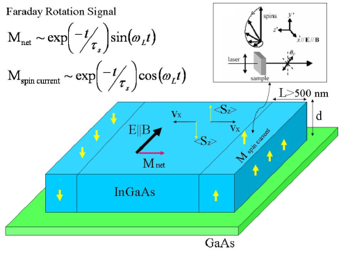
Figure 2: An electric field will cause both an observed net uniform bulk magnetization and a proposed spin current. The spin current will accumulate at the edges over a spin diffusion length of more than $500nm$ thus making its detection practical with a beam slightly more focused than in kato2 . The uniform magnetization and the spin current spin accumulatio are $\pi/2$ out of phase.

Finally, using the current setup in kato1 ; kato2 we propose an experiment to test the prediction of dissipationless spin current. For spin 1/2 two-dimensional systems, the initial prediction sinova is subject to some sort of controversy, Inoue:2003 ; halperin ; nomura as the introduction of impurities apparently makes the spin current vanish. We here adopt the alternative view and propose a clear-cut experiment which can see the spin accumulation due to the spin current. Similar to the 2D case, in the present case, the application of an electric field $E_{j}$ to a semiconductor with spin orbit coupling will create a spin current $S_{l}^{i}$ flowing perpendicular to the electric field and polarized perpendicular to both the field and the direction of flow. Using linear response, the expression for the spin conductance is:

$$\\ J_{i}^{l}=\sigma_{ij}^{l}E_{j}\\ \sigma_{ij}^{l}=\frac{\hbar^{2}}{2m}\int\frac{d^{3}k}{(2\pi)^{3}}\frac{n_{E_{-}}-n_{E_{+}}}{B^{3}}k_{i}\epsilon_{lnm}B_{n}\frac{\partial B_{m}}{\partial k_{j}}$$ (7)

where $i,j,l,m,n=x,y,z$, $\epsilon_{lnm}$ is the totally antisymmetric tensor in 3 dimensions and $B_{i}(k)$ are the components of the internal magnetic field. For $H_{3}$ and for $\epsilon_{xx}=\epsilon_{yy}$ the only non-zero components of the spin conductance are:

$$\sigma^{3}_{21}=-\sigma^{3}_{12}=\frac{e}{\hbar}\frac{1}{D(\epsilon_{zz}-\epsilon_{yy})}\frac{\hbar^{2}}{m}\int\frac{d^{3}k}{(2\pi)^{3}}\frac{n_{E_{-}}-n_{E_{+}}}{(k_{x}^{2}+k_{y}^{2})^{3/2}}k^{2}_{y}=\\ =\frac{e}{\hbar}\frac{1}{D(\epsilon_{zz}-\epsilon_{yy})}\frac{\hbar^{2}}{2m}\frac{1}{(2\pi)^{3}}\int_{0}^{2\pi}d\phi\int_{0}^{\pi}d\theta\sin^{2}{\phi}(k_{-}^{2}-k_{+}^{2})$$ (8)

where $\phi,\theta$ are the polar angles of $\overrightarrow{k}$ and where $k_{-},k_{+}$ are the fermi momenta of the two bands. When both bands are occupied (positive Fermi energy), we find $k_{-}-k_{+}=\frac{2m}{\hbar^{2}}\frac{\lambda(k)}{k},\;\lambda(k)=D(\epsilon_{zz}-\epsilon_{xx})k\sin\theta$. Usually the spin splitting is much smaller than the Fermi energy, and we can define an average Fermi momentum $k_{F}=\frac{1}{2}(k_{-}+k_{+})\approx(3\pi^{2}n)^{1/3}$, $n$ being the dopant density. With this, we find that the spin-conductivity will be independent of the value of the strain:

$$\sigma^{3}_{21}=-\sigma^{3}_{12}=\frac{e}{\hbar}\frac{k_{f}}{4\pi^{2}}$$ (9)

The result for the spin conductance is intermediate between the 2D spin 1/2 spin current and the 3D spin 3/2 spin current. Similar to murakami1 but unlike sinova the spin conductance depends on the fermi momentum, a characteristic of the 3D. Unlike murakami1 , but similar to sinova , the spin conductance does not depend on the strength of spin-orbit coupling. Even though the spin conductance does not depend on the value of strain, it is essential that spin-orbit splitting (due to strain in this case) be present. Upon the application of an electric field on the $x$ axis, a spin current will flow on the $y$ axis spin polarized in the $z$ direction. For $n=10^{16}cm^{-3}$, and a field $E=10^{4}V/m$ we estimate a spin current $j_{spin}=\frac{e}{\hbar}\frac{k_{f}}{4\pi^{2}}E=2\times 10^{21}(\mu_{B}/cm^{2}s)$ where $\mu_{B}$ is a Bohr magneton. Since spin conductivity varies as $n^{\frac{1}{3}}$ and charge conductivity varies as $n$, for low values of $n$ the spin conductance will overtake the charge conductance and the spin current will be larger than the charge current caused by the electric field. The density at which this happens is $n^{2/3}<\frac{2e}{\hbar\mu}\frac{(6\pi^{2})^{1/3}}{8\pi^{2}}$, where $\mu$ is the mobility in the sample, or $n<2\times 10^{16}cm^{-3}$ for a sample of mobility $\mu=0.6m^{2}/Vs$.

The flow will result in accumulation on the opposite $zx$ faces of the crystal (see Fig[2]). For the present experiment, we estimate this spin accumulation of the order of $J_{spin}\tau_{S}=10^{13}\mu_{B}/cm^{2}$. Due to the extremely spin life time of above $1ns$, the distance from the edge of the sample, the spin diffusion length is very large, of the order $L=500nm-1\mu m$. The FR beam used in kato2 has a resolution of $4.7\mu m/9.7\mu_{m}$ on the x and y axis respectively, but focusing the beam within $1\mu m$ is possible kato4 ; stephens . Then, if the spin current prediction is right, applying the FR beam on the edge of the sample should give a clear signal (larger than the uniform magnetization in the bulk). Since the uniform magnetization and the spin accumulation due to spin hall current are perpendicular to each other, in time-resolved FR experiments, the spin current spin accumulation and the uniform magnetization are out of phase by $\pi/2$ (see Fig[2)

In conclusion, we have analyzed two very recent experiments kato1 ; kato2 and proved that conventional spin splitting terms and strain spin splitting terms do not explain the data. We have introduced a previously largely unknown term and made the case as to why it explains the observed features in kato1 ; kato2 . We have proposed further simple experiments to verify our assertions. If true, our proposal gives rise to the clear possibility of obtaining a uniform magnetization parallel to the applied electric field, as opposed to the one perpendicular to it that has been observed so far. Along with predicting a 3D spin current, we have also proposed a way to test the spin currents in spin 1/2 systems.

BAB wishes to primarily thank Y. Kato for many essential discussions and explanations regarding the experiments kato1 ; kato2 . The authors also wish to thank H. Manoharan for many stimulating discussions on strain-related issues and E. Mukamel for critical discussions relating to the experiments kato1 ; kato2 . Many thanks also go to G. Zeltzer, L. Souza De Mattos for discussions on strain growth and H.D. Chen for useful technical support. B.A.B. acknowledges support from the Stanford Graduate Fellowship Program. This work is supported by the NSF under grant numbers DMR-0342832 and the US Department of Energy, Office of Basic Energy Sciences under contract DE-AC03-76SF00515.

References

- (1) Y. Kato et al., Nature 427, 50 (2004)
- (2) Y. Kato et al., cond-mat 0403407
- (3) S.A. Wolf et al, Science 294, 1488 (2001).
- (4) S. Murakami, N. Nagaosa, and S.C. Zhang, Science 301, 1348 (2003)
- (5) J. Sinova et al, cond-mat 0307663, to appear in Phys. Rev. Lett.
- (6) M. I. Dyakonov and V. I. Perel, Phys. Lett. A 35, 459 (1971).
- (7) J. E. Hirsch, Phys. Rev. Lett. 83, 1834 (1999).
- (8) S. Zhang, Phys. Rev. Lett. 85, 393 (2000).
- (9) L. S. Levitov, Y. V. Nazarov, and G. M. Eliashberg, Sov. Phys. JETP 61, 133 (1985).
- (10) V. M. Edelstein, Solid State Commun. 73, 233 (1990).
- (11) A. G. Aronov, Y. B. Lyanda-Geller, and G. E. Pikus, Sov. Phys. JETP 73, 537 (1991).
- (12) L. I. Magarill, A. V. Chaplik, and M. V. Entin, Semiconductors 35, 1081 (2001).
- (13) A. V. Chaplik, M. V. Entin, and L. I. Magarill, Physica E 13, 744 (2002).
- (14) J. Inoue, G. E. W. Bauer, and L. W. Molenkamp, Phys. Rev. B 67, 33104 (2003).
- (15) X. Cartoixa, D. Z. Y. Ting, E. S. Daniel, and T. C. McGill, Superlattices Microstruct. 30, 309 (2001).
- (16) R. H. Silsbee, Phys. Rev. B 63, 155305 (2001).
- (17) S.D. Ganichev et al., cond-mat 0403641
- (18) Y. Kato et al., Nature 427, 50 (2004), Supplementary Strain Table
- (19) K.L. Kavanagh et al., J. Appl. Phys. 64, 4843 (1988)
- (20) Y. Kato, private communication
- (21) We thank Y. Kato for revealing this point to us.
- (22) S. Datta and B. Das, Appl. Phys. Lett. 56, 665 (1990)
- (23) G.E. Pikus and A.N. Titkov, Optical Orientation (North-Holland, Amsterdam, 1984), p.73
- (24) I. Vurgaftman et al., J. Appl. Phys. 89, 5815 (2001)
- (25) T. Hassenkam et al. Phys. Rev. B 55, 9298 (1997)
- (26) W. Howlett and S. Zukotynski, Phys. Rev. B 16, 3688 (1977)
- (27) A.V. Khaetskii and Y. V. Nazarov, Phys. Rev. B. 64, 125316 (2001)
- (28) T.B. Bahder, Phys. Rev. B. 41, 11992 (1990)
- (29) D.G. Seiler, B.D. Bajaj and A.E. Stephens, Phys. Rev. B. 16, 2822 (1977)
- (30) M.I. D’yakonov et al., Zh. Eksp. Teor. Fiz 90, 1123 (1986) [Sov. Phys. JETP 63, 655 (1986)]
- (31) D. Culcer et al., cond-mat/0408020
- (32) G.C. La Rocca et al., Phys. Rev. B 38, 7595 (1988)
- (33) E.G. Mishchenko, A.V. Shytov, B.I. Halperin, cond-mat/0406730
- (34) K. Nomura et al. cond-mat/0407279
- (35) J. Stephens et al., cond-mat/0401197, Phys. Rev. B 68, 41307(R)(2003)