Kinetics of propagating phase transformation in compressed bismuth

Abstract

We observed dynamically driven phase transitions in isentropically compressed bismuth. By changing the stress loading conditions we explored two distinct cases: one in which the experimental signature of the phase transformation corresponds to phase-boundary crossings initiated at both sample interfaces, and another in which the experimental trace is due to a single advancing transformation front in the bulk of the material. We introduce a coupled kinetics - hydrodynamics model that for this second case enables us, under suitable simplifying assumptions, to directly extract characteristic transition times from the experimental measurements.

The kinetics of first-order phase transformations has long been a topic of great experimental and theoretical interest gms83 ; lt73 . Phase separation is, for example, a common technologically important occurrence in many alloys fpl99 , while structural-transition kinetics is believed to be relevant for understanding the dynamics of Earth’s mantle ss94 . The development of high pressure experimental techniques has brought new perspectives on this problem, and new insights on long-standing scientific puzzles, e.g. the formation of natural diamond ouk04 . Understanding the kinetics of high pressure phase transitions is also an important step in fulfilling the promise of high pressure science to help develop new materials for technological applications pm02 . Dynamic compression experiments allow the study of such non-equilibrium processes occurring on very short timescales - $10^{-12}$ to $10^{-6}s$, which are otherwise difficult to investigate with traditional, static high pressure techniques. We present here the results of isentropic compression experiments exploring non-equilibrium behavior associated with polymorphic phase transitions in bismuth.

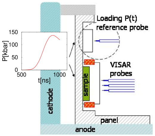
Figure 1: Schematic cross-section through target assembly. Bi sample is contained between the panel (Cu or Al) and the transparent window (LiF or Sapphire). Heat is applied to the sample through a band heater (red) wrapped around the circumference of the window. A 3 mm vacuum gap (AK gap) exists between the panel and cathode. A rapidly varying magnetic field in the AK gap generates the pressure pulse that compresses the Bi sample. A reference probe assembly consisting of a transparent window impedance matched and glued to the panel provides a direct measurement of the loading pressure profile for each sample - see inset P(t).

The experiments were carried out using high purity poly-crystalline bismuth samples shaped as disks with $8-10mm$ diameter and $0.3-0.6mm$ thickness, with very flat and parallel surface finish obtained by diamond turning. The initial conditions were ambient pressure and temperatures between $\simeq 300K$ and $\simeq 400K$, where bismuth has a well studied rhombohedral crystal structure - Bi(I). We applied a smooth, magnetically driven pressure ramp to the target containing the sample - see Fig. 1 for the experimental set-up, with duration of $\simeq 300ns$ and $\simeq 150kbar$ maximum value. As a result the system was driven along a quasi-isentropic thermodynamic path that first crosses the Bi(I) phase boundary into the Bi(II) phase, with a centered monoclinic crystal structure. We measured the time dependence of the velocity of the interface between the sample and a transparent window using velocity interferometry technique (VISAR) VISAR . The loading pressure was carefully designed to avoid developing shocks in the sample before the phase transformation conditions were achieved, and monitored in each experiment with a reference probe. The details of the magnetic pulse generation are similar with the ones described in ice-tech . To insure high accuracy results the initial temperature variation across the sample diameter was continuously monitored, and was found to be $\leq 5K$. Also, the velocity of the sample/window interface was measured on several points, spaced up to 2 mm apart, each traced with 1-2 interferometers with different sensitivities to eliminate fringe loss uncertainties. The windows used in the experiments were [100] single crystal lithium fluoride - $LiF$ and sapphire. Their optical properties in the pressure-temperature regime accessed in these experiments are summarized in win1 ; win2 .

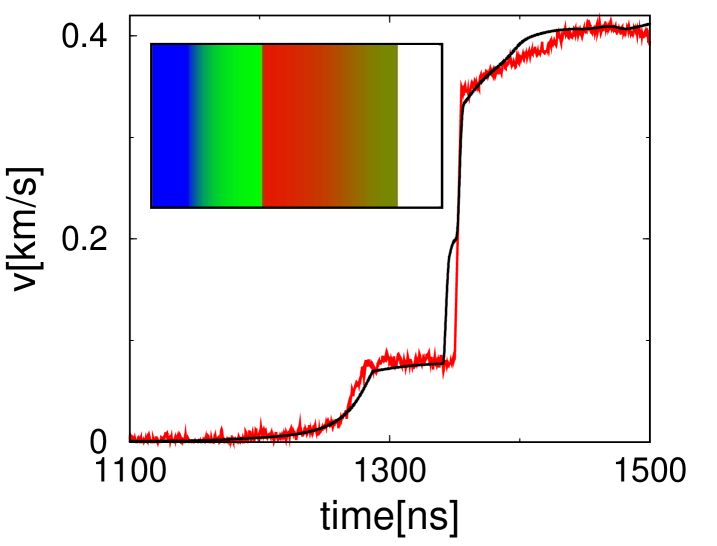
Figure 2: VISAR trace (interface velocity) for the sapphire window experiment: red line; hydrodynamic simulations: black line. Inset: color-coded lateral cross section through the sample-window assembly showing the phase transformation fronts originating at the loading interface (left) and sapphire window (right) - Bi(I) (red), Bi(II)(green), Bi(III)(blue), sapphire (white) at $t\simeq 1310ns$.

The behavior of bismuth during these experiments can be partly understood by comparing the sample/window interface velocity traces - $v(t)$, with the results of standard, equilibrium, one-dimensional hydrodynamic simulations. We performed such calculations using a multi-phase bismuth equation of state derived from the free energy model of Ref. hayes-Bi-EOS , which describes very well the phases of main interest here - Bi(I) and Bi(II), and the position of their phase boundary; the higher pressure phase - Bi(III) is represented with lower accuracy, but that should not alter our conclusions. To insure accurate modeling the panels and windows were also included and described by Mie-Gruneisen equations of state Marsh . The maximum densities achieved for bismuth were $\simeq 12.8g/cm^{3}$ and the temperatures were below $\simeq 550K$. The simulation results indicate that upon compression a structural phase transformation from the initial Bi(I) rhombohedral structure to the Bi(II) centered monoclinic structure (with a $5\%$ volume collapse) is initiated at $\simeq 19-24kbar$ and $\simeq 320-410K$, depending on the initial conditions. The transition is signaled in both experiments and simulations by a change in the slope of $v(t)$ - see Figs. 2 and 3, which is followed in the simulations by a velocity “plateau”; similar effects have been observed in shock experiments dg77 . Due to the complex wave interactions associated with the presence of material interfaces the pressure distribution inside the sample, and therefore the position dependent thermodynamic paths followed, are directly dependent on the compressive properties of the window.

In the case of the sapphire window both the inception of the plateau and the measured velocity value, $\simeq 0.07km/s$, agree well with the hydrodynamic calculations, Fig. 2. A detailed analysis of the simulation results reveals that the transformation is initiated both at the loading-interface, due to the applied pressure, and at the back-interface, due to the pressure enhancement created by the “hard” (higher dynamic impedance) sapphire window, resulting in two transformation fronts traveling in opposite directions - see inset to Fig.2. The start of the non-accelerating regime (velocity plateau) corresponds to the beginning of the phase transformation at the back-interface, while its end and the sharply rising velocity mark the completion of the transition in the entire sample.

For the case of the $LiF$ window on the other hand the experimental traces show surprisingly large deviations from the simulations. A softer window such as LiF creates a slight depressurization at the sample/window interface. Equilibrium hydrodynamic simulations indicate that the transformation front initiated at the loading-interface is traveling through the sample largely undisturbed by the back-interface. The velocity plateau starts when the perturbation generated by the advancing transformation reaches the interface, and is a thermodynamic equilibrium effect. No such plateau is observed in the experiment, although a marked change in acceleration, $\partial v/\partial t$, is present, see Fig. 3. This transient regime ends as before upon completion of the phase transition in the entire sample, as shown by the hydrodynamic calculations.

In order to understand these results we consider the effect of solid-solid phase transition kinetics on dynamically driven phase transformations. In the present experiments bismuth undergoes a reconstructive structural first-order phase transformation, the kinetics of which can be described by a simple picture of nucleation and growth originally proposed by Kolmogorov k37 . This model is currently known as the Kolmogorov-Johnson-Mehl-Avrami (KJMA) model jm39 ; a41 ; c73 , and it has been employed to describe a variety of systems edkg94 ; kpng98 ; kg01 ; blct04 ; we recall the main ideas below. For other, more detailed models of nucleation and growth see also loc92 .

If the system, initially in thermodynamic equilibrium in phase 1, is suddenly forced, e.g. by increasing the pressure, into the phase 2 region of its phase diagram, infinitesimally small domains of the stable phase will occur uniformly throughout the sample with a nucleation rate per unit volume $\gamma(t)$. Once formed the domains grow isotropically with constant interface velocity $u$, i.e. the rate of volume growth of a domain is assumed proportional with its surface area. At a later time $t$ the radius of a nucleus generated at $t\prime$ will be $r(t-t\prime)=u\times(t-t\prime)$, and its volume growth rate $w(t-t\prime)=4\pi u^{3}(t-t\prime)^{2}$. Therefore the unimpeded growth rate of the volume fraction of phase 2, $\phi_{2}$, will be $W(t)=\int_{0}^{t}w(t-t\prime)\gamma(t\prime)dt\prime$. However, the growth of the 2-nd phase can only occur in the volume still occupied by the 1-st phase, $1-\phi_{2}$, and as a result the actual growth rate is assumed proportional with $W$ and the volume still available. If at $t\rightarrow\infty$ the two phases coexist in thermodynamic equilibrium with volume fractions $\phi^{0}_{1}$ and $\phi^{0}_{2}$, the available volume is only $\phi^{0}_{2}-\phi_{2}$, and the rate of change of $\phi_{2}$ is:

$$\frac{\partial\phi_{2}}{\partial t}=(\phi^{0}_{2}-\phi_{2})W(t)$$ (1)

This equation can be easily integrated if the system is not externally driven, e.g. by varying the applied pressure, i.e. $\phi^{0}_{2}$ is constant in time:

$$\phi_{2}(t)=\phi^{0}_{2}\left\{1-\exp\left[-\int_{0}^{t}W(t\prime)dt\prime\right]\right\}$$ (2)

Two simple cases of the above equation have been often studied. One corresponds to time independent nucleation rate, also known as homogeneous nucleation. The other describes a situation where the nucleation process occurs primarily on defects, e.g. grain boundaries, or impurities already present in the sample, i.e. heterogeneous nucleation. In particular if the preexisting nucleation sites are assumed randomly distributed in the system with a number density $\gamma_{0}$ this formally corresponds to Eq. 1 with $\gamma(t)=\gamma_{0}\delta(t)$. In both cases Eq. 1 reduces to:

$$\phi_{2}(t)=\phi^{0}_{2}\left\{1-\exp{\left[-\left(\frac{t}{\tau}\right)^{n}\right]}\right\}$$ (3)

where the kinetic time constant is $\tau\propto(\gamma u^{3})^{-\frac{1}{4}}$ for homogeneous nucleation, and $\tau_{0}\propto(\gamma_{0}u^{3})^{-\frac{1}{3}}$ for heterogeneous nucleation. For the homogeneous case $n=4$ and $n=3$ for the heterogeneous one. However, $n$ can be interpreted more generally as a measure of the effective dimensionality of domain growth, which for heterogeneous nucleation in particular can be smaller than $3$, as first discussed by Cahn c56 .

The modeling of the dynamic compression experiments described here requires the coupling of the transformation kinetics Eq. 1 with appropriate macroscopic conservation equations for mass, momentum and energy, i.e. hydrodynamic equations. We now introduce a model and analysis that capture the effect of phase transformation kinetics on the propagation of perturbations through the system, and allow a quantitative interpretation of the experimental results.

Consider a semi-infinite sample in thermodynamic equilibrium at temperature $T$, coexistence pressure $P_{c}$ and density $\rho_{1}$ corresponding to the lower density phase. We are interested in the behavior of the system under a small perturbation, e.g. slight uniaxial compression with frequency $\nu$. If we neglect heat exchange processes, i.e. assume that the flow is isentropic, only mass and momentum conservation equations - Euler equations llfm - need to be considered. Together with Eq. 1 they constitute our coupled kinetics-hydrodynamics model. For small enough density and velocity deviations from equilibrium linearized Euler equations are sufficient, and read:

$$\frac{\partial\rho}{\partial t}=-\rho_{1}\frac{\partial v}{\partial z}$$ (4)

$$\frac{\partial v}{\partial t}=-\frac{1}{\rho_{1}}\frac{\partial p}{\partial z}$$ (5)

Eqs. 1,4 and 5 describe the propagation of small, long wavelength perturbations in the phase coexistence region of the phase diagram. To make further progress we use instead of Eq. 1 the integrated form Eq. 3, which should not introduce large errors since we expect that $\phi^{0}_{2}$ is a slow, hydrodynamic variable, which changes on time scales of order $\nu^{-1}$ ($\nu^{-1}\simeq 500ns$ in the experiment), much larger than the characteristic time scale of Eq. 1, i.e. $\nu^{-1}\gg\tau$. As usual this set of equations needs to be closed by expressing the pressure $p$ as a function of density $\rho$ and volume fraction $\phi_{2}$, as well as $\phi^{0}_{2}$ as function of $\rho$, all at constant entropy. We assume here that thermal as well as mechanical equilibrium prevail on time scales much shorter than $\tau$ in microscopically large but macroscopically small sample regions, for arbitrary local volume fractions $\phi_{2}$ of the coexisting phases. We also introduce further simplifying assumptions, for example that the differences between the densities and compressibilities of the two phases are small - e.g. they are $\simeq 5\%$ for bismuth I and II, and also that differences between the isentrope and an average isotherm are small, which holds well for bismuth at the typical experimental pressures and temperatures. We obtain for the velocity equation:

$$\frac{\partial v}{\partial t}=-\frac{\chi_{1}}{\rho_{1}^{2}}\left(\frac{\partial\rho}{\partial z}\right)exp{\left[-\left(\frac{t-t_{0}}{\tau}\right)^{n}\right]}$$ (6)

$t\geq t_{0}$, where $\chi_{1}$ is the adiabatic compressibility of phase 1 and $t_{0}$ is the arrival time of the compressive perturbation at position $z$. In conjunction with Eq. 4 the above relation yields a modified sound equation for the density. Guided by the experimental set-up, where the compression starts below the transition line, we argue that the density variations propagate approximately as sound waves with the frequency $\nu$ of the applied perturbation. Since we assume $\nu^{-1}\gg\tau$, we can therefore write for the velocity equation:

$$\frac{\partial v}{\partial t}\simeq A(z)exp{\left[-\left(\frac{t-t_{0}}{\tau}\right)^{n}\right]}$$ (7)

$t\geq t_{0}$, where $A(z)$ (defined by comparison with Eq. 6) is now time independent. For reasonably short time intervals $\delta t=t-t_{0}$ this equation should approximately govern the evolution of the velocity not too far ahead of the transformation front.

We expect the above analysis, corresponding to a propagating transformation front in the vicinity of the phase line, to be suitable for the “soft” LiF window experiments. For this case we would therefore like to fit the experimentally measured back-interface velocity with the functional form Eq. 7, to obtain information on the effective kinetic time constant $\tau$ and the Avrami exponent $n$. To this end we set $t_{0}$ by comparing with instantaneous kinetics hydrodynamic calculations and restrict the fit to approximately one-half of the duration of the reduced acceleration regime, to avoid the effects of pressure reverberation between the transformation front and the LiF window. Coincidentally, the fit termination point can also be identified as an inflection point. A typical result is shown in Fig. 3, where we find $\tau\simeq 24ns$. This reasonably validates a posteriori the assumption of a scale separation between $\tau$ and $\nu^{-1}$. We determine an Avrami exponent $n\simeq 1.3$, which suggests strongly heterogeneous nucleation dominated by a high density of sites located on grain interfaces c56 . This is consistent with the poly-crystalline character of the bismuth samples used in the present experiments. For the “hard” sapphire window on the other hand, an additional transformation front is generated at the sample/window interface due to pressure enhancement at that boundary. This occurs before the arrival of sound waves from the forward moving transformation front and thereby obscures its effect.

As shown before, in the case of heterogeneous nucleation the characteristic time constant $\tau$ depends on the density of defects $\gamma_{0}$ and the phase interface velocity $u$; $\gamma_{0}$ is directly related to the average size of the grains for the case of grain boundary nucleation, while the interface motion is driven by both thermodynamical forces - the difference between the chemical potential of the two phases $\Delta\mu$, and mechanical ones - the applied loads and the elastic stresses that occur at the boundary between the competing phases due to their different densities and lattice structures fr98 ; vil02 . In the vicinity of the phase line the thermodynamical contribution to $u$ has a fairly simple form dt56 ; lai02 , $u\propto\lambda\Delta\mu\exp(-Q/k_{B}T)$, where $\lambda$ is the interface thickness and $Q$ the activation energy for atomic cross-interface motion; here $\Delta\mu$ should be interpreted as a time-averaged chemical potential difference. If we neglect the pressure dependence of $\lambda$ and $\Delta\mu$ (the phase line is to a good approximation flat) and assume that the exponential term contains the dominant temperature contribution, for similar samples crossing the phase line at different thermodynamic points the time constants $\tau$ should reflect an Arrhenius-type temperature dependence of the interface velocity. For LiF window experiments at transition temperatures $T_{1}\simeq 320K$, $T_{2}\simeq 360K$ and $T_{3}\simeq 410K$ we find $\tau$’s consistent with such a behavior, and an activation energy $Q\simeq 0.2eV$. Although the interplay between thermodynamical and mechanical forces is rather complex lhsa04 , this suggests that the thermodynamic force is dominant, at least in the initial stages of transformation kinetics.

We believe that our experimental results and analysis provide new insight on phase transformation kinetics occurring under dynamic conditions, and open the possibility of experimentally designing and characterizing both thermodynamic and kinetic paths.

This work was performed under the auspices of the U. S. Department of Energy by University of California Lawrence Livermore National Laboratory under Contract No. W-7405-Eng-48.

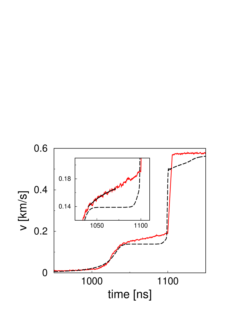
Figure 3: VISAR trace (interface velocity) for a LiF window experiment: red line; hydrodynamic simulations: dashed black line. Inset: blow-up of the reduced acceleration regime and kinetics fit (see text): solid black line.

References

- (1) For a review, see J.D. Gunton, M. San Miguel, and P.S. Sahni, in Phase Transitions and Critical Phenomena, edited by C. Domb and J.L. Lebowitz (Academic, London, 1983), vol. 8.
- (2) J.S. Langer, L.A. Turski, Phys. Rev. A 8, 3230 (1973).
- (3) P. Fratzl, O. Penrose, J.L. Lebowitz, J. Stat. Phys. 95, 1429 (1999).
- (4) V.S. Solomatov, D.J. Stevenson, Earth Planet. Sci. Lett. 125, 267 (1994).
- (5) T. Okada, W. Utsumi, H. Kaneko, V. Turkevich, N. Hamaya, and O. Shimomura, Phys. Chem. Minerals 31, 261 (2004).
- (6) P.F. McMillan, Nature Materials 1, 19 (2002).
- (7) L. Barker, R. Hollenbach, J. Appl. Phys. 43, 4669 (1972).
- (8) C.A. Hall, J.R. Asay, M.D. Knudson, W.A. Stygar, R.B. Spielman, T.D. Pointon, D.B. Reisman, A. Toor, and R.C. Cauble, Rev. Sci. Instr. 72, 3587 (2001).
- (9) D.B. Hayes, C.A. Hall, J.R. Asay, and M.D. Knudson, J. Appl. Phys. 94, 2331 (2003).
- (10) L. Wise, L.C. Chhabildas, in Shock Waves in Condensed Matter, edited by Y.M. Gupta (Plenum, New York, 1986), p. 441.
- (11) D.B. Hayes, J. Appl. Phys. 46, 3438 (1975).
- (12) S.P. Marsh, LASL Shock Hugoniot Data (University of California Press, Berkeley, 1980).
- (13) G.E. Duvall, R.A. Graham, Rev. Mod. Phys. 49, 523 (1977).
- (14) A.N. Kolmogorov, Bull. Acad. Sci. U.S.S.R., Phys. Ser. 3, 555 (1937).
- (15) W.A.. Johnson, R.F. Mehl, Trans. Am. Inst. Min. Metall. Pet. Eng. 135, 416 (1939).
- (16) M. Avrami, J. Chem. Phys. 7, 1103 (1939); 8, 212 (1940); 9, 177 (1941).
- (17) J.W. Christian, The Theory of Transformations in Metals and Allows, second edition, (Pergamon, Oxford, 1973), chapter 2.
- (18) K.R. Elder, F. Drolet, J.M. Kosterlitz, and M. Grant, Phys. Rev. Lett. 72, 677 (1994).
- (19) M. Karttunen, N. Provatas, T. Ala-Nissila, and M. Grant, J. Stat. Phys. 90, 1401 (1998).
- (20) M.D. Knudson, Y.M. Gupta, J. Appl. Phys. 91, 9561 (2002).
- (21) F. Berthier, B. Legrand, J. Creuze, and R. Tetot, J. Electroanal. Chem. 562, 127 (2004).
- (22) M. Lin, G.B. Olson, M. Cohen, Metall. Trans. A 23A, 2987 (1992).
- (23) J.M. Cahn, Acta Metall. 4, 449 (1956).
- (24) See, for example, L.D. Landau, E.M. Lifshitz, Fluid Mechanics, second edition, (Butterworth-Heinemann, Oxford, 1987).
- (25) F.D. Fischer, G. Reisner, Acta Mater. 46, 2095 (1998).
- (26) V.I. Levitas, Int. J. Plasticity 18, 1499 (2002).
- (27) D. Turnbull, in Solid State Physics, edited by F. Seitz and D. Turnbull (Academic, London, 1956), Vol. 3, p. 225.
- (28) For a more recent analysis see V.I. Levitas, A.V. Idesman, G.B. Olson, and E.N. Stein, Phil. Mag. A 82, 429 (2002).
- (29) V.I. Levitas, B.F. Henson, L.B. Smilowitz, and B.W. Asay, Phys. Rev. Lett. 92, 235702 (2004).