Coherent electronic transport in a multimode quantum channel
with Gaussian-type scatterers

Abstract

Coherent electron transport through a quantum channel in the presence of a general extended scattering potential is investigated using a $T$-matrix Lippmann-Schwinger approach. The formalism is applied to a quantum wire with Gaussian type scattering potentials, which can be used to model a single impurity, a quantum dot or more complicated structures in the wire. The well known dips in the conductance in the presence of attractive impurities is reproduced. A resonant transmission peak in the conductance is seen as the energy of the incident electron coincides with an energy level in the quantum dot. The conductance through a quantum wire in the presence of an asymmetric potential are also shown. In the case of a narrow potential parallel to the wire we find that two dips appear in the same subband which we ascribe to two quasi bound states originating from the next evanescent mode.

I Introduction

In studies of electronic transport in mesoscopic or nanoscale quasi-one-dimensional systems it has strikingly been found that the conductance manifests quantization B. J. van Wees et al. (1988a); D. A. Wharam et al. (1988); B. J. van Wees et al. (1988b); van Houten et al. (1989) when the electronic phase-coherent length $l_{\phi}$ is greater than the system size. The transport properties of these systems have been successfully described within the Landauer-Büttiker framework. Landauer (1957, 1970, 1992); Buttiker et al. (1985); Buttiker (1986, 1988) Later on, the influence of a single impurity on the conduction in quantum channels has attracted a great deal of attention since the impurity inside or near the conducting channel may destroy the conduction quantization, as has been demonstrated theoretically  Chu and Sorbello (1989); P. F. Bagwell (1990); Tekman and Ciraci (1991); Nixon et al. (1991); Y. B. Levinson et al. (1992); Takagaki and Ferry (1992); Kunze and Lenk (1992); Chu and Chou (1994); Boese et al. (2000) and experimentally. Faist et al. (1990)

The impurities are usually assumed to be zero-range, i.e. of a delta-function type, in theoretical considerations.P. F. Bagwell (1990); V. Vargiamidis and O. Valassiades (2002); G. Cattapan and E. Maglione (2003) However, a real physical impurity must be of finite range and therefore modeled by an extended potential. In this paper we discuss coherent transport properties of quantum channels in the presence of extended scattering potentials. If the potentials are very extended they can describe the effects of a tunable central gate.Soh et al. (2001)

The method for the coherent electron transport through the quantum channel employs the Lippmann-Schwinger (LS) formalism. Its relation to the $T$-matrix and the Landauer formula in terms of elements of the scattering matrix is discussed in Sec. II. The conductance of a quantum channel in the presence of extended Gaussian type scattering potentials obtained by numerical calculations is given in Sec. III. This section consists of three parts. First we discuss the scattering by a single Gaussian potential. The physics of the transport is examined more closely by visualizing the most important processes by help of the LS equation. In the second part we model a quantum dot embedded in the wire by a combination of two Gaussian potentials, and use that to obtain the conductance of such a setup. The effect of the shape of an extended scattering potential on the conductance is considered in the last part. In Sec. IV we summarize and discuss the main results of the paper.

II Scattering by a Potential

We consider a quantum wire connected adiabatically to reservoirs as schematically shown in Fig. 1. The uniformity of the wire is broken by a scattering potential of finite extent in the wire.

Figure 1: Schematic view of the system. An incoming wave is partly transmitted and partly reflected by the finite range scattering potential $V$.

The wave function of a single-electron state with energy $E$, in the quasi-one-dimensional quantum wire is described by the Schrödinger equation

$$\left(-\frac{\hbar^{2}}{2m}\left[\frac{\partial^{2}}{\partial x^{2}}+\frac{\partial^{2}}{\partial z^{2}}\right]+V_{c}(x)+V(\mathbf{r})\right)\psi_{E}(\mathbf{r})=E\psi_{E}(\mathbf{r}).$$ (1)

The electron is confined in the $x$-direction by the confinement potential $V_{c}(x)$ but is free to propagate in the $z$-direction. $V(\mathbf{r})$ is a finite range scattering potential. The transverse modes

$$\left(-\frac{\hbar^{2}}{2m}\frac{d^{2}}{dx^{2}}+V_{c}(x)\right)\chi_{n}(x)=\varepsilon_{n}\chi_{n}(x),$$ (2)

are assumed to be known.

Outside the range of the scattering potential an electron with energy $E$ is in a linear combination of the eigenfunctions of $H_{0}=H-V(\mathbf{r})$. These eigenfunctions are referred to as modes and can be written

$$\phi_{nE}^{\pm}(\mathbf{r})=\frac{1}{\sqrt{k_{n}(E)}}e^{\pm ik_{n}(E)z}\chi_{n}(x),$$ (3)

where $E=\hbar^{2}k_{n}^{2}(E)/2m+\varepsilon_{n}$ and the modes are normalized to carry unit probability current.Fisher and Lee (1981); Henrik Bruus and Karsten Flensberg (2002) The $+$ (-) refers to waves incident from the left (right). If $\varepsilon_{n}<E$, $k_{n}(E)$ is real and $\phi_{nE}^{\pm}$ are propagating waves (see Fig. 2). If on the other hand $\varepsilon_{n}>E$, $k_{n}(E)$ is purely imaginary and the eigenfunctions must be exponentially decaying, evanescent modes.

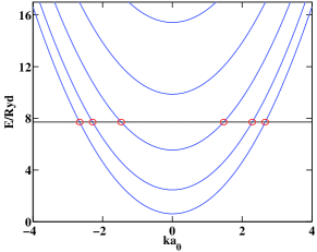
Figure 2: (Color online). The energy levels of a quantum wire with a hard wall confinement. For a given energy $E$ (horizontal line) only a finite number of propagating modes are active (red markers), but higher lying evanescent modes can serve as intermediate states. This specific case is for a wire of width $L=4a_{0}$. Energy is scaled in Rydbergs (Ryd) and lengths in Bohr radii ($a_{0}$), cf. Sec. III.

Scattering states are special solutions of Eq. (1), where e.g. an electron in propagating mode $n$ impinges on the scattering potential from the left and is backscattered or transmitted into other modes. In the far zone, outside the range of the scattering potential, the scattering states have the boundary condition

$$\psi_{nE}^{+}(\mathbf{r})=\begin{cases}\phi_{nE}^{+}(\mathbf{r})+\sum_{m,\text{prop}}r_{mn}\phi_{mE}^{-}(\mathbf{r}),&z\rightarrow-\infty,\\ \sum_{m,\text{prop}}t_{mn}\phi_{mE}^{+}(\mathbf{r}),&z\rightarrow\infty.\end{cases}$$ (4)

$t_{mn}$ is the probability amplitude for a particle in mode $n$ in the left lead to scatter out in mode $m$ in the right lead. $r_{mn}$ gives the probability amplitude for reflection into mode $m$. By restricting all the modes to carry unit current the transmission amplitudes coincide with the elements of the scattering matrix.Buttiker et al. (1985) Hence, the zero temperature linear response conductance of the system can be obtained by the Landauer formula Buttiker et al. (1985); Fisher and Lee (1981)

$$G=\frac{2e^{2}}{h}\text{Tr}[t^{\dagger}t],$$ (5)

where the matrix of the transmission amplitudes $t$ is evaluated at the Fermi energy.

II.1 Scattering States and the Lippmann-Schwinger Equation

We expand the scattering states in the transverse modes

$$\psi_{nE}^{+}(\mathbf{r})=\sum_{m}\varphi_{mE}^{n}(z)\chi_{m}(x),$$ (6)

where the $n$ denotes the number of the incident mode (cf. Eq. (4)). Introducing this expansion in the Schrödinger equation (1), multiplying with $\chi_{m^{\prime}}^{*}(x)$, integrating over $x$ and letting $m\leftrightarrow m^{\prime}$, one obtains a coupled mode equationP. F. Bagwell (1990); G. Cattapan and E. Maglione (2003)

$$\left(\frac{d^{2}}{dz^{2}}+k_{m}^{2}(E)\right)\varphi_{mE}^{n}(z)=\frac{2m}{\hbar^{2}}\sum_{m^{\prime}}V_{mm^{\prime}}(z)\varphi_{m^{\prime}E}^{n}(z),$$ (7)

where

$$V_{mm^{\prime}}(z)=\int dx\,\chi_{m}^{*}(x)V(\mathbf{r})\chi_{m^{\prime}}(x).$$ (8)

Defining a mode Green’s function as

$$\left(\frac{d^{2}}{dz^{2}}+k_{n}^{2}(E)\right)\mathcal{G}_{nE}^{0}(z,z^{\prime})=\delta(z-z^{\prime}),$$ (9)

the solution to Eq. (7) can be written in the form of an effective 1D LS equation

$$\begin{split}\varphi_{mE}^{n}(z)&=\varphi_{mE}^{n0}(z)+\frac{2m}{\hbar^{2}}\sum_{m^{\prime}}\int dz^{\prime}\,\mathcal{G}_{mE}^{0}(z,z^{\prime})\\ &\times V_{mm^{\prime}}(z^{\prime})\varphi_{m^{\prime}E}^{n}(z^{\prime}),\end{split}$$ (10)

where $\varphi_{mE}^{n0}(z)=\delta_{nm}\exp(ik_{m}(E)z)/\sqrt{k_{m}(E)}$. Note that the solutions of the LS equation (10) obey the same normalization as the incident mode. Inserting the explicit form of the Green’s function,

$$\mathcal{G}_{nE}^{0}(z,z^{\prime})=-\frac{i}{2k_{n}(E)}e^{ik_{n}(E)|z-z^{\prime}|},$$ (11)

in Eq. (10) and taking the limit $z\rightarrow\infty$, one obtains by comparison with Eq. (4) the probability amplitudes for forward scattering

$$\begin{split}t_{mn}&=\delta_{mn}+\frac{m}{i\hbar^{2}}\sum_{m^{\prime}}\int dz^{\prime}\,\frac{1}{\sqrt{k_{m}(E)}}e^{-ik_{m}(E)z^{\prime}}\\ &\times V_{mm^{\prime}}(z^{\prime})\varphi_{m^{\prime}}^{n}(z^{\prime}).\end{split}$$ (12)

II.2 Scattering States and the $T$-matrix

Having obtained the transmission amplitudes in terms of the configuration space wave function we now find them in terms of matrix elements of a transition operator. Inserting the definition (8) of $V_{mm^{\prime}}$ into relation (12) and using the expansion (6) one obtains

$$t_{mn}=\delta_{mn}+\frac{m}{i\hbar^{2}}\langle mk_{m}|\hat{V}|\psi_{nE}^{+}\rangle,$$ (13)

where in general $\langle\mathbf{r}|nq\rangle=(\exp(iqz)/\sqrt{|q|})\chi_{m}(x)$. Similarly, using the LS equation (10) in the same expansion, we see that

$$\begin{split}\psi_{nE}^{+}(\mathbf{r})=\phi_{nE}^{+}(\mathbf{r})+\int d^{3}r^{\prime}\,\mathcal{G}_{0}(\mathbf{r},\mathbf{r}^{\prime};E)V(\mathbf{r}^{\prime})\psi_{nE}^{+}(\mathbf{r}^{\prime})\end{split}$$ (14)

where

$$\mathcal{G}_{0}(\mathbf{r},\mathbf{r}^{\prime};E)=\frac{2m}{\hbar^{2}}\sum_{m}\chi_{m}^{*}(x)\mathcal{G}_{mE}^{0}(z,z^{\prime})\chi_{m}(x).$$ (15)

This is just the conventional LS equation and therefore by defining the $T$-matrix by the relation

$$\langle mk^{\prime}|\hat{T}|nk_{n}\rangle=\langle mk^{\prime}|\hat{V}|\psi_{nE}^{+}\rangle,$$ (16)

it satisfies the operator LS equation

$$\hat{T}=\hat{V}+\hat{V}\hat{\mathcal{G}}_{0}(E)\hat{T}.$$ (17)

In the eigenfunction basis of $\hat{H}_{0}$ the LS equation (16) is transformed intoG. Cattapan and E. Maglione (2003)

$$\begin{split}T_{mn}(k,k_{n})&=V_{mn}(k,k_{n})+\frac{m}{\pi\hbar^{2}}\sum_{l}\int dq\,|q|\\ &\times\frac{V_{ml}(k,q)T_{ln}(q,k_{n})}{k_{l}^{2}-q^{2}+i\eta},\end{split}$$ (18)

where the notation $V_{ml}(k,q)=\left\langle mk\right|\hat{V}\left|lq\right\rangle$ has been introduced. We have used that in our current normalization the unity operator is

$$\hat{1}=\sum_{l}\int dq\,\frac{|q|}{2\pi}\left|lq\right\rangle\left\langle lq\right|,$$ (19)

and that the Green’s function is

$$\left\langle lq\right|\hat{\mathcal{G}}_{0}(E)\left|l^{\prime}q^{\prime}\right\rangle=\frac{2\pi}{|q|}\frac{\delta_{ll^{\prime}}\delta(q-q^{\prime})}{E-\frac{\hbar^{2}q^{2}}{2m}-\varepsilon_{l}+i\eta}.$$ (20)

The numerical solution of Eq. (18) is briefly discussed in App. A.

In the above notation the transmission amplitudes can be written

$$t_{mn}=\delta_{mn}+\frac{m}{i\hbar^{2}}T_{mn}(k_{m},k_{n}).$$ (21)

Note that through Eq. (18) $T_{mn}(k_{m},k_{n})$ depends on $T$-matrix elements both on and off the energy shell ($\hbar^{2}k^{2}/2m+\varepsilon_{n}$ is equal to $E$ on the energy shell but not off it).

We have thus managed to link the elements of the transmission matrix to matrix elements of the transition operator $\hat{T}$. The result is intuitively appealing, transmission from one channel to another is related to the transition from an eigenstate in one channel to an eigenstate in another. The formalism is quite general with respect to the type of wire confinement and scattering potential of finite range. A change of either one requires only a new evaluation of matrix elements of the scattering potential and the energy spectrum of $H_{0}$.

III Results

In our model we use two potentials, one describing the confinement and the other representing the scattering potential. We use two different models for either one of these. The confining potential, characterizing the extent of the quantum channel, can be described by either a hard wall potential

$$V_{c,\text{hard}}(x)=\begin{cases}0&0<x<L\\ \infty&\text{elsewhere},\end{cases}$$ (22)

with eigenvalues $\varepsilon_{n}=\hbar^{2}\pi^{2}(n/L)^{2}/2m$, $n=1,2,\ldots$, or parabolic walls

$$V_{c,\text{parabolic}}(x)=\frac{1}{2}m\omega^{2}x^{2}r,$$ (23)

with eigenvalues $\varepsilon_{n}=(n+1/2)\hbar\omega$, $n=0,1,\ldots$. Note that the first mode in the hard wall confinement has $n=1$ but $n=0$ in the parabolic case.

By a proper choice of model for the scattering potential one can study a multitude of different systems. In the following subsections we will by use of Gaussian functions model a single impurity by a single Gaussian, a quantum dot embedded in the wire by a sum of two Gaussians of different size and finally study shape effects of the scattering potential by asymmetric Gaussians. Even though we have chosen to use only Gaussian potentials we stress that the formalism is general and can be used with more complicated potentials. By cleverly choosing the functional form of the scattering potential it can be adapted to describe many experimental setups.

In this paper we scale all energies in Rydbergs (Ryd) and lengths in units of Bohr radii ($a_{0}$). The calculations are independent of exact material constants but it can be useful to keep in mind that in GaAs $a_{0}=9.79$ nm and Ryd $=5.93$ meV.

III.1 Single Gaussian Potential

A single Gaussian potential

$$V(\mathbf{r})=V_{0}e^{-\alpha((x-x_{i})^{2}+z^{2})}.$$ (24)

can be used to model an impurity in the wire or the effect of a tunable central gate.Soh et al. (2001) In this subsection and the ones that follow, the center $(x_{i},0)$ of the potential is chosen to be in the middle of the wire (i.e. $x_{i}=L/2$ and $x_{i}=0$ in the hard wall and parabolically confined quantum wires respectively) unless otherwise noted.

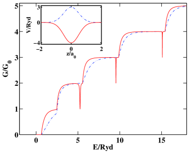
Figure 3: (Color online). Conductance of a hard wall quantum wire in units of $G_{0}=2e^{2}/h$ as a function of energy in the presence of a single repulsive (dashed, $V_{0}=3$ Ryd, $\alpha=2a_{0}^{-2}$) and attractive (solid, $V_{0}=-4$ Ryd, $\alpha=2a_{0}^{-2}$) Gaussian scattering potential. The inset shows the scattering potentials in a cross section along the middle of the wire ($x=L/2$). The total number of modes is $N=8$. The width of the wire is $L=4a_{0}$.

The conductance of a hard wall quantum wire in the presence of such a Gaussian scatterer is shown in Fig. 3. In the case of a repulsive potential, the well known steps in the conductance are little smeared out, similar to what is seen in experiments.B. J. van Wees et al. (1988a) One should remember though that our calculations are at zero temperature, so there is no temperature smearing. In experiments, the finite temperature can be a significant source of smearing of the steps. Additionally, in the case of an attractive potential, there are dips in the conductance right before the onset of the next mode. The dips can be understood from a simple coupled mode model to be due to backscattering by a quasi-bound state originating from an evanescent mode in the next energy subband.S. A. Gurvitz and Y. B. Levinson (1993); P. F. Bagwell (1990) A more general explanation in terms of the symmetries of the scattering matrix also exist. J. U. Nöckel and A. D. Stone (1994) This effect is a multimode effect that disappears if evanescent modes are not included in the calculations. Interestingly, there is no dip in the first subband. This can also be understood from the coupled mode model, in which coupling between the first propagating mode and the quasi-bound state in the first evanescent mode is given by $V_{12}(z)$. Due to symmetry this matrix element is zero, the potential being even and the wave functions for the first and second transverse modes being even and odd respectively, hence no dip.

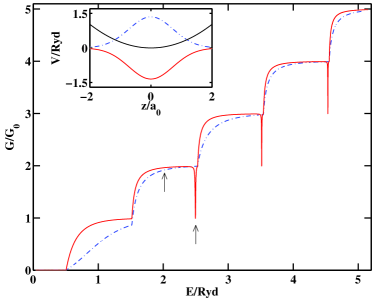
Figure 4: (Color online). Conductance of a parabolic quantum wire in units of $G_{0}=2e^{2}/h$ as a function of energy in the presence of a single repulsive (dashed, $V_{0}=1.35$ Ryd, $\alpha=0.96a_{0}^{-2}$) and attractive (solid, $V_{0}=-1.35$ Ryd, $\alpha=0.96a_{0}^{-2}$) Gaussian scattering potential. The inset shows the scattering potentials in a cross section along the middle of the wire ($x=0$) and the parabolic confinement potential ($\hbar\omega=1.01$ Ryd). The total number of modes is $N=9$. The arrows point at the the energies at which the probability density is calculated in Figs. 5 and 6.

The conductance of a parabolic wall quantum wire in the presence of a single Gaussian scattering potential is shown in Fig. 4. Due to different dependence of the transverse energy levels on the subband number (linear and square) the length of the plateaus increases in the case of hard wall potential while being of constant length for the parabolic wires. Besides this, there is no qualitative difference between the two confinement potentials.

The conductance of the hard wall quantum wires has been obtained by solving for the $T$-matrix through Eq. (18). The conductance of the parabolic wall quantum wire has both been obtained by the $T$-matrix approach and by solving the real space LS Eq. (10). In the latter case the real space wave function is a part of the solution but has to be calculated separately in the $T$-matrix case (cf. App. B). Visualizing the wavefunctions can aid in discussing the scattering processes. Therefore, we now visually examine the system of the parabolically confined wire at the energies marked by an arrow in Fig. 4, making the physics of the process more clear.

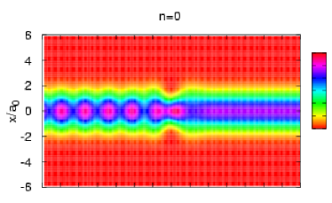
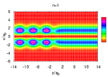
Figure 5: (Color online). The probability density of the scattering states $\psi_{nE}^{+}$ in the parabolic quantum wire in the presence of the single attractive Gaussian scattering potential of Fig. 4. The total energy of the incident particle is $E=2.02$ Ryd (cf. the left arrow in Fig. 4). The incoming wave is in mode $n=0$ (above) and $n=1$ (below).

In Fig. 5 we have plotted the probability density $|\psi_{nE}^{+}(\mathbf{r})|^{2}$ of the scattering state for incoming waves with $n=0$ and $n=1$, at the energy indicated by the left arrow in Fig. 4.

The incoming wave is partly reflected and partly transmitted. To the left of the scattering center the incoming part and the reflected part interfere to form the beating pattern seen. To the right, only the transmitted part exists and the probability density is independent of $z$. It is interesting to note that in general the transmitted part in the second subband is a linear combination of the first two modes. The two modes should then interfere to make a beating pattern also on the right hand side. However, as already mentioned, the coupling between the first two modes is zero due to symmetry. Therefore an incident electron in the first mode cannot be transmitted into the second mode. Examining a similar picture in the third subband reveals interference between mode $n=0$ and mode $n=2$ in the right hand side, in agreement with the above. The effect of the normal modes can also be seen in the nodal structure in the transverse direction. The second mode, $n=1$, has a node in the middle of the wire while the first mode, $n=0$, is nodeless.

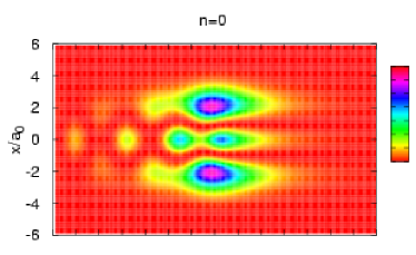
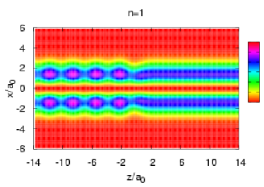
Figure 6: (Color online). The probability density of the scattering states $\psi_{nE}^{+}$ in the parabolic quantum wire in the presence of the single attractive Gaussian scattering potential of Fig. 4. The total energy of the incident particle is $E=2.50$ Ryd, coinciding with a dip in the conductance (cf. the right arrow in Fig. 4). The incoming wave is in mode $n=0$ (above) and $n=1$ (below).

More interesting things are happening in the dip in the second subband. The upper panel of Fig. 6 shows the probability density of the scattering state obtained when the incident wave is in mode $n=0$. This mode is resonantly backscattered due to coupling to an evanescent state in mode $n=2$. Mode $n=1$ is unaffected because of symmetry blocking (lower panel of Fig. 6). The evanescent state with the corresponding nodal structure is clearly seen in the total wavefunction as a localized state around the scattering potential. A beating pattern to the left of the scattering center, similar to the one seen in Fig. 5, due to the interference of the incoming and reflected wave is faintly seen. On the other side of the potential, however, no outgoing wave is seen in agreement with resonant backscattering. An incident wave in mode $n=1$ can due to symmetry not couple to the evanescent state. A scattering state with such an incident wave is thus expected to be qualitatively the same as for an energy away from the dip in the same subband, as can be seen in the lower panel of Fig. 6. The main difference between the scattering states with incident wave in mode $n=1$ in Fig. 5 and Fig. 6 is that the latter is at higher energy. The wave vector is thus higher, resulting in higher frequency in the oscillations of the probability density, The same is true when comparing the different frequencies of the oscillations in the two cases of Fig. 5. In the $n=0$ case, a smaller part of the energy is in the transverse mode thus increasing the wave vector of the wave in the propagating direction.

Both of these effects, the steps and the dip, are well known in the literature. However, in most calculations the scattering potential is of zero-range delta function type.P. F. Bagwell (1990); V. Vargiamidis and O. Valassiades (2002); G. Cattapan and E. Maglione (2003) Extended potentials are rare, an example being the rectangle potential of Bagwell.P. F. Bagwell (1990) An interesting difference can be seen in the total number of modes needed in the calculations. In our case, 8 modes give results that change insignificantly if more modes are added. In the delta function case, up to 100 modes are needed, a clear signature of the singular nature of the delta function potential.

III.2 A Quantum Dot Embedded in the Wire

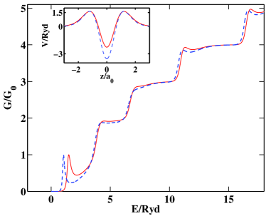
Figure 7: (Color online). Conductance of a hard wall quantum wire in units of $G_{0}=2e^{2}/h$ as a function of energy in the presence of a double Gaussian scattering potential with a varying depth of the well. The inset shows the scattering potentials, whose parameters in the solid (dashed) case are $V_{1}=5.21$ ($6.16$) Ryd, $V_{2}=7.49$ ($9.70$) Ryd, $\alpha_{1}=0.52$ ($0.60$) $a_{0}^{-2}$ and $\alpha_{2}=1.52$ ($1.60$) $a_{0}^{-2}$, in the cross section $x=L/2$. The total number of modes is $N=8$. The width of the wire is $L=4a_{0}$.

The double Gaussian

$$V(\mathbf{r})=V_{1}e^{-\alpha_{1}r^{2}}-V_{2}e^{-\alpha_{2}r^{2}}\quad\alpha_{2}>\alpha_{1},$$ (25)

can be used to model a quantum dot embedded in the wire. The conductance of a hard wall quantum wire with such a quantum dot is given in Fig. 7. Compared to the single impurity, a new effect appears. An enhanced conductance in the first subband along with similar weaker structures in higher bands. This is the well known effect of resonant tunneling. A remnant of a bound state in the well induces a resonance in the transmission, hence the resonance in the conductance.

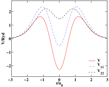
Figure 8: (Color online). The solid line represents the double Gaussian potential of Fig. 7 along with its first two effective potentials.

Examining the coupled mode equation (7), one notices that, ignoring the coupling between the modes, the transmission is governed by the effective potentials $V_{nn}(z)$. In Fig. 8 we have plotted the double Gaussian potential along with its first two effective potentials. We know from resonant tunneling in 1D, that the higher the probability for the electron to tunnel out of the well, the broader the resonance in the transmission. The difference in the sharpness of the tunneling resonances in different subbands can therefore be attributed to the different shapes of the effective potential.

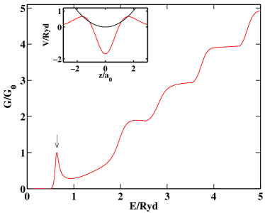
Figure 9: (Color online). Conductance of a parabolic wall quantum wire in units of $G_{0}=2e^{2}/h$ as a function of energy in the presence of a double Gaussian scattering potential. The inset shows the scattering potential, whose parameters are $V_{1}=2.02$ Ryd, $V_{2}=3.71$ Ryd, $\alpha_{1}=0.29$ $a_{0}^{-2}$ and $\alpha_{2}=0.96$ $a_{0}^{-2}$, in the cross section $x=0$. The parabolic confinement potential ($\hbar\omega=1.01$ Ryd) is also shown. The total number of modes is $N=9$. The arrow points at the value of the energy at which the probability density in Fig. 10 is calculated.

The conductance through a quantum dot in a parabolic wire in Fig. 9 has the same pronounced resonance in the first subband but the resonances in the higher subbands are even more suppressed than in the hard wall wire.

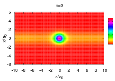
Figure 10: (Color online). The probability density of the scattering states $\psi_{nE}^{+}$ in the parabolic quantum wire in the presence of the double Gaussian scattering potential of Fig. 9. The total energy of the incident particle is $E=0.64$ Ryd, coinciding with a resonance in the conductance (cf. the arrow in Fig. 9). The incoming wave is in mode $n=0$.

The resonant tunneling is through the remnants of a bound state in the well. In contrast to the resonant backscattering, this quasi-bound state belongs to the propagating subband, not the next evanescent mode. The resonance is thus not a multimode phenomenon as the dip certainly is. We examine the probability density in the most pronounced resonance of Fig. 9, that is the one marked by an arrow. There is only one propagating mode and thus the only scattering state is the one with an incident wave in mode $n=0$; the probability density of which is shown if Fig. 10. The quasi-bound state in the middle of the wire is clearly seen. The absence of beating on both sides of the scattering center indicates that there is no reflected wave, i.e. the incoming wave is perfectly transmitted. This supports very well the suggestion that the resonance is due to resonant tunneling through a remnant of a bound state in the well.

III.3 Shape Effects of the Scattering Potential

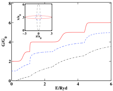
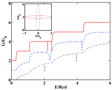
Figure 11: (Color online). Conductance of a hard wall quantum wire in units of $G_{0}=2e^{2}/h$, as a function of energy. A single contour of the scattering potential, an asymmetric single Gaussian, is shown in the inset. The contour is chosen to be at the value of $V_{0}e^{-1}=0.368V_{0}$. In the upper panel the potentials are repulsive ($V_{0}=3$ Ryd) but attractive ($V_{0}=-3$ Ryd) in the lower panel. In both cases the circularly symmetric potential has $\alpha=2$ $a_{0}^{-2}$, the transverse one has $\alpha_{x}=0.10$ $a_{0}^{-2}$ and $\alpha_{z}=6.73$ $a_{0}^{-2}$, and the longitudinal has $\alpha_{x}=9.10$ $a_{0}^{-2}$ and $\alpha_{z}=0.11$ $a_{0}^{-2}$. The parameters are chosen such that the volume between the potential and the zero energy plane are equal. The width of the wire is $L=6$ $a_{0}$ and the total number of modes is $N=8$. The symmetric and longitudinal potentials have been shifted by $1$ $G_{0}$ and $2$ $G_{0}$ respectively, for clarity.

So far, the scattering potentials under examination have all been circularly symmetric. Elongated extended scattering potentials, such as the asymmetric Gaussian

$$V(\mathbf{r})=V_{0}e^{-\alpha_{x}(x-x_{i})^{2}-\alpha_{z}z^{2}},$$ (26)

offer more variety. The conductance characteristics for the cases of elongated longitudinal, elongated transverse, and circularly symmetric potential profiles are under investigation, as shown in Fig. 11. The parameters of the potentials have been chosen such that their volume in the wire is the same in all cases. This is done so that the strength of the scatterers is comparable in all cases. We have used both attractive and repulsive potentials.

We begin by discussing the conductance of the repulsive potentials in the upper panel of Fig. 11. The conductance of the transverse barrier is lower than its circularly symmetric counterpart. The conductance of the longitudinal barrier has a more pronounced exponential growth and is thus lower than the conductance of the circularly symmetric barrier at the low energy part of each subband while being higher in the high energy end. Both the symmetric and the longitudinal barrier are mainly confined to the middle of the wire. Modes that have nodes in the middle of the wire, i.e. the second, fourth etc. mode, see very little of the potential and go easily through. This is especially clear in the case of the longitudinal potential were these modes have almost perfect transmission as soon as they become propagating. The transverse barrier is nearly independent of the transverse direction and affects all the modes equally.

The lower panel of Fig 11 shows the conductance of attractive potentials. Compared to the symmetric case, the elongated longitudinal and transverse attractive barriers have higher and lower conductance respectively. The dip structure is quite different. The shape of the dips in the transverse case are more of the asymmetric Fano form than the more common Breit-Wigner form as in the longitudinal case.J. U. Nöckel and A. D. Stone (1994) In the longitudinal case, we have two dips rather than the usual single dip. Because of symmetry blocking, there are no dips in the first band as before. Even though no dips are seen in the third subband we belive they are there. They are just to narrow to be seen in the energy resolution of the calculations.

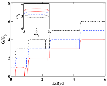
Figure 12: (Color online). Conductance of a hard wall quantum wire in units of $G_{0}=2e^{2}/h$, as a function of energy. The scattering potential has the same parameters as the attractive potential in Fig. 11, but the center is moved from the middle of the wire $x_{i}=L/2$ to $x_{i}=5L/8$ and $x_{i}=3L/4$. The width of the wire is $L=6$ $a_{0}$ and the total number of modes is $N=8$ as before. The inset shows the $V_{0}e^{-1}$ contour of the scattering potentials. The potentials in the center of the wire and the one with $x_{i}=5L/8$ have been shifted by $1$ $G_{0}$ and $2$ $G_{0}$ respectively, for clarity.

The dips are most probably too narrow to be seen in experiments. By shifting the center of the potential from the middle of the wire, dips in the first subband are no longer blocked (cf. Fig. 12). When the center of the longitudinal potential is in $x_{i}=3L/4$ we have two dips that are quite pronounced. We will now focus on these two dips.

If we include only one mode, i.e. the propagating mode, in the calculations these dips disappear. Both dips reappear by adding just the first evanescent mode. The higher evanescent modes change the conductance curve only quantitatively, shifting the dips and affecting their width. We therefore deduce that both dips can be explained by a coupled mode model restricted to two modes. This kind of model as already been put forth to explain the single dip in the presence of a single impurity.S. A. Gurvitz and Y. B. Levinson (1993); J. U. Nöckel and A. D. Stone (1994) Nöckel and Stone noted that a quasi-bound state $\Phi$, satisfying

$$\left(-\frac{\hbar^{2}}{2m}\frac{d^{2}}{dz^{2}}+V_{22}(z)\right)\Phi(z)=(E_{0}-\varepsilon_{2})\Phi(z)$$ (27)

appears from the evanescent mode. They note that there is no need for the dip to be close to the subband edge. Even though they do not mention it, it is apparent from their formalism that there is also nothing that prevents more than one quasi-bound state to be present, as long as there are more than one solution to Eq. (27) with $E_{0}-\varepsilon_{2}<0$. We therefore suggest that the two dips are due to two quasi-bound states originating from the first evanescent mode. To confirm this suggestion we have solved Eq. (27) numerically by putting a large box around the potential and expanding the bound state $\Phi$ in the plane-wave eigenfunctions of the particle in a box with periodic boundary conditions. The energy eigenvalues obtained are plotted in Fig. 13, showing clearly that there are two bound states, that develop into quasi-bound states due to coupling to the propagating state.

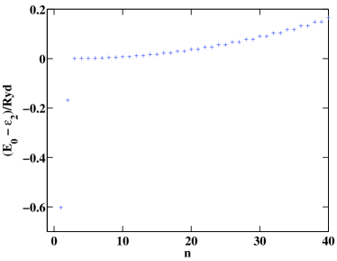
Figure 13: The energy levels of the effective potential $V_{22}(z)$ of the longitudinal attractive potential of Fig. 12 with $x_{i}=3L/4$. The levels are obtained in a box of length $L_{\text{box}}=150$ $a_{0}$.

Depending on the shape and strength of the scattering potential the above argument suggests that one could see even more dips in each subband. Furthermore, if the binding energy fulfills $E_{0}-\varepsilon_{2}<-(\varepsilon_{2}-\varepsilon_{1})$, a true bound state originating from the second mode would exist.

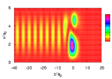
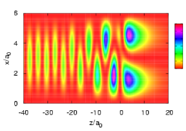
Figure 14: (Color online). The probability density of the scattering states $\psi_{nE}^{+}$ in the hard wall quantum wire in the presence of the elongated longitudinal Gaussian potential shown in the inset of Fig. 12 shifted to $x_{i}=3L/4$. The incident wave is in mode $n=1$ and has total energy $E=0.865$ ($1.084$) Ryd in the upper (lower) panel. These energies correspond to the two dips in the conductance of Fig. (12).

To confirm our suggested mechanism, in Fig. 14, we examine the probability density of the scattering states at the energies corresponding to the two dips. The symmetries of the quasi-bound states are as expected. The one lower in energy is nodeless in the $z$ direction while the other one has a single node. Both have the symmetry of the transverse mode $n=2$.

We note in passing that the width of the scattering potential can be estimated as the width of the $V_{0}e^{-1}$ contour. The elongated potential in Fig 12 has the width $0.33$ $a_{0}$ in the transverse direction and $3.02$ $a_{0}$ in the propagating $z$ direction. We observe that the quasi-bound states are much more extended than one would expect of a true bound state in the potential. They also have probability density on both sides of the wire. The above indicates that we are looking at the two quasi-bound states from mode $n=2$.

IV Summary and discussion

In this work we have studied the coherent quantum transport in the presence of various realistic Gaussian-type scattering potentials using the Lippmann-Schwinger $T$-matrix approach. We have calculated the conductance and the spatial distribution of the electron probability and their dependence on the shape of the scattering potentials. The formalism is quite general and can be applied to quantum wires modeled with different confinement potentials, and in the presence of a general extended scattering potential. We have used both hard wall confinement and parabolically confined quantum wires. The scattering potential has been modeled by Gaussian potential, using single and double, symmetric and asymmetric Gaussians. By a combination of these we have modeled a single impurity, a quantum dot embedded in the wire and studied the shape effects of the scattering potential. Repulsive impurity smooths out the exact quantization of the conductance while attractive impurity shows the well known dips in the conductance. A resonant transmission appears in the conductance through the quantum dot as the energy of the incident electron coincides with an energy level in the dot. A longitudinal barrier affects modes of different symmetry differently while a transverse barrier affects all the modes in the same way. In an attractive longitudinal potential two dips can appear in the same subband. These two dips appear due to coupling of a propagating mode to two quasi-bound states that both originate in the next evanescent mode.

Our calculations demonstrate the power and flexibility of the current approach. Being able to calculate the conductance of a quantum wire in the presence of a general extended scattering potential allows for a multitude of systems to be studied. Our Gaussian potentials are rather simple but by appropriately choosing the scattering potential many different experimental setups can be modeled.

Appendix A Solving the $T$-matrix Integral Equation

When solving the LS equation for the $T$-matrix, Eq. (18), numerically, one has to treat the singularities of the Green’s function with care. By using the fact that

$$\frac{1}{k_{l}^{2}-q^{2}+i\eta}=\frac{{\cal P}}{k_{l}^{2}-q^{2}}-\frac{i\pi}{2k_{l}}\left(\delta(q-k_{l})+\delta(q+k_{l})\right),$$ (28)

the integral on the right hand side can be transformed into two algebraic terms plus a principal value integral (${\cal P}$ denotes a principal value)

$${\cal P}\int_{-\infty}^{\infty}dq\,\frac{V_{ml}(k,q)T_{ln}(q,k_{n})}{k_{l}^{2}-q^{2}}.$$ (29)

Since

$${\cal P}\int_{0}^{\infty}dq\,\frac{1}{k_{l}^{2}-q^{2}}=0,$$ (30)

it is possible to remove the singularity of the integrand by a subtraction of a zero M. I. Haftel and F. Tabakin (1970); Rubin H. Landau (1996). For a general function $f$ we have (assuming $k>0$)

$$\begin{split}{\cal P}&\int_{-\infty}^{\infty}dq\,\frac{f(q)}{k_{l}^{2}-q^{2}}={\cal P}\int_{0}^{\infty}dq\,\frac{f(-q)+f(q)}{k_{l}^{2}-q^{2}}=\\ &\int_{0}^{\infty}dq\,\frac{f(-q)-f(-k_{l})}{k_{l}^{2}-q^{2}}+\int_{0}^{\infty}dq\,\frac{f(q)-f(k_{l})}{k_{l}^{2}-q^{2}}.\end{split}$$ (31)

The value of the integrand at the singularity can, by use of l’H$\hat{\text{o}}$pital’s rule, be seen to be $\mp f^{\prime}(\pm k)/2k$. Assuming that $f^{\prime}$ is nonsingular at $\pm k$, the principal value can therefore be skipped as already done. Using this prescription and numerical Gaussian integration for the remaining integrals, the integral LS equation for the $T$-matrix is transformed into a system of linear equations that can be solved by standard linear algebra methods.Bardarson (2004)

The Green’s function for the evanescent modes is non singular since $k_{l}^{2}<0$. The integral in Eq. (18) for evanescent modes is therefor done with numerical Gaussian integration without the above special treatment for singularities.

Appendix B Scattering states in terms of the T-matrix

By a spectral representation of the mode Green’s function, Eq. (9),

$$G_{mE}^{0}(z,z^{\prime})=\frac{1}{2\pi}\int_{-\infty}^{+\infty}dp\frac{e^{ip(z-z^{\prime})}}{k_{m}^{2}-p^{2}},$$ (32)

the wave function in Eq. (10) can be rewritten as

$$\begin{split}\phi_{mE}^{n}(z)&=\phi_{mE}^{n0}(z)+\frac{m}{\pi\hbar^{2}}\sum_{m^{\prime}}\int_{-\infty}^{+\infty}dp\frac{e^{ipz}}{k_{m}^{2}-p^{2}}\\ &\times\iint dx^{\prime}dz^{\prime}e^{-ipz^{\prime}}\chi_{m}^{*}(x^{\prime})V(\mathbf{r}^{\prime})\phi_{m^{\prime}E}^{n}(z^{\prime})\chi_{m^{\prime}}(x^{\prime}),\end{split}$$ (33)

which further yields

$$\begin{split}\phi_{mE}^{n}(z)&=\phi_{mE}^{n0}(z)+\frac{m}{\pi\hbar^{2}}\int_{-\infty}^{+\infty}dp\frac{\sqrt{|p|}e^{ipz}}{k_{m}^{2}-p^{2}}\\ &\times\iint dx^{\prime}dz^{\prime}\frac{e^{-ipz^{\prime}}}{\sqrt{|p|}}\chi_{m}^{*}(x^{\prime})V(\mathbf{r}^{\prime})\Psi_{nE}^{+}(\mathbf{r}^{\prime}),\end{split}$$ (34)

where we have used the expansion in Eq. (6). By the definition of the T-matrix, Eq. (16), we can thus rewrite Eq. (34) as

$$\begin{split}\phi_{mE}^{n}(z)=\phi_{mE}^{n0}(z)+\frac{m}{\pi\hbar^{2}}\int_{-\infty}^{+\infty}dp\frac{\sqrt{|p|}e^{ipz}}{k_{m}^{2}-p^{2}}T_{mn}(p,k_{n}).\end{split}$$ (35)

We have thus expressed the wave function in terms of the elements of the T-matrix. By Eq. (35) and the expansion in Eq. (6) we are able to determine the scattering states $\Psi_{nE}^{+}$ for all $\mathbf{r}$. In the case of propagating modes, the singularities of the mode Green’s function are treated the same way as in App. A. For evanescent modes there are no singularities and we furthermore have that the incoming wave, $\phi_{mE}^{n0}(z)$, is zero.