Separation of plastic deformations in polymers
based on elements of general nonlinear theory

Abstract

We report a method for describing plasticity in a broad class of amorphous materials. The method is based on nonlinear (geometric) deformation theory allowing the separation of the plastic deformation from the general deformation tensor. This separation allows an adequate pattern of thermodynamical phenomena for plastic deformations in polymers to be constructed. A parameter, $\theta$ describing the stress relaxation rate of the material is introduced within the frame of this approach. Additionally, several experimental configurations to measure this parameter are discussed.

Plastic and elastic deformation plays a critical role in the description of physical phenomena in Earthis crustal deformations E.  L. Geist, D. J. Andrews [2000], transfer of slurry, powdery and granular materials through pipelines S. J. Fiedor, J. M. Ottino [2003], and, especially, in polymer dynamics P.  G. de Genes [1990]. Although the theory of elastic deformation including elastic equilibrium, deflection and torsion of rods, bending of plates and shells is a classical and well developed field, a completed theory applied to plastic media is yet to be developed.

The theories describing microscopic plastic deformations in metals is based on a born-death dislocation mechanism producing a shift of crystallographic grid. This have been developed by E. Orowan, M. Polanyi, G. I. Taylor, J. M. Burgers, F. C. Frank, W. T. Read, R. E. Pierels, P. B. Hirsch, W. C. Dash, Yu. A. Osipyan et al (J.  P. Hirth, J. Lothe [1968]). In solids, the shear transformation zone theory (STZ) has been developed by Falk and Langer M. L. Falk, J. S. Langer , A. E. Lobovsky, J. S. Langer . However, a complete theory of plastic deformation in polymer materials has not developed so far. Physical behavior of polymers at the nanoscale is important from the fundamental point of view to understand deformation processes, evolution of homogeneous or heterogeneous nanostructures, and the thermal history of monomer architecture D. R. Heine, G. S. Grest, E. B. Webb , M. Akai-Kasaya, K. Shimizu, Y. Watanabe, A. Saito, M. Aono, Y. Kuwahara . Understanding the deformation behavior in polymers would eventiually produce novel nanostructure formation techniques based on nano-deformations.

Polymers are probably most suitable materials in which plastic deformation can be studied experimentally. Recently, Lyuksyutov and Vaia with co-authors reported nanopattering technique based on localized Joule heating of a thin polymer films S. F. Lyuksyutov, R. A. Vaia, P. B. Paramonov, S. Juhl, L. Waterhouse, R. M. Ralich, G. Sigalov, E. Sancaktar , S. F. Lyuksyutov, P. B. Paramonov, S. Juhl, R. A. Vaia . A biased atomic force microscope (AFM) tip produces an electric current flow through the polymer film resulting in localized Joule heating of the polymer above its glass transition temperature due to electronic breakdown through the film. Polarization and electrostatic attraction of softened polymer toward the AFM tip in the presence of a strong ($10^{9}$-$10^{10}$ Vm^-1) non-uniform electric field produce raised or depressed nanostructures (10-50 nm width, and 0.1-100 nm height) in a broad class of polymers of different physical-chemical properties. This technique, named AFM-based electrostatic nanolithography (AFMEN), can be applied to the study of plastic deformations since both a liquid and a plastic solid polymer phases coexist during the process. The breakdown during AFMEN is a critical factor causing film softening, and polymer mass transfer as a result. Recent experimental data indeed produce the evidence of nanostructure formation in polymer that cannot be explained by the electronic breakdown. The most likely reason for polymer nanostructure formation when an AFM tip of 20-50 nm in diameter moves above the surface is the plastic deformation of polymer molecules through triboelectrification mechanism. No electronic breakdown is required to deform the polymer surface in this case. An exact analytical solution, based on the method of images, has been obtained for the description of the electric field between an atomic force microscope (AFM) tip and a thin dielectric polymer film (30 nm thick) spin-coated on a conductive substrate. Three different tip shapes are found to produce electrostatic pressure above the plasticity threshold in the polymers up to 50 MPa S. F. Lyuksyutov, P. B. Paramonov, R. A. Sharipov, and G. Sigalov . Should such a technique, based on plastic deformations in polymer materials, be developed further, it would create an alternative to existing nanopattering techniques effective tool, for patterning on nanoscale. There has been a lot of activity in in last few years in developing these techniques including: 1) direct resist lithography developed by Schaeffer et al E. Schaffer, T. Thurn-Albrecht, T. Russel, and U. Steiner based on the competition of Van der Waal’s and Laplace forces on polymer-air interface in strong electric field; and 2) hierarchic nanostructure formation based on electrodynamic instability in bilayer polymer films developed by Russell et al M. D. Morariu, N. A. Voicu, E. Schaeffer, Z. Lin, T. P. Russell, and U. Steiner . The only industrial prototype for nanostructure formation in polymers called MILLIPEDE developed by Vettinger et al P. Vettiger, M. Despont, U. Drechsler, U. Durig, W. Haberle, M. I. Lutwyche, H. E. Rothuizen, R. Stutz, R. Widmer, G. K. Binning is based on thermal-mechanical lithography developed by Mamin and Rugar yearlier in the 90s. H. J. Mamin, D. Rugar . The authors of the MILLIPEDE project predict a replacement of ferromagnetic memories with based on polymers in the next 20 years.

Experimental verification of the existence of plastic deformation on nanoscale in AFM-tip-polymer-metal system S. F. Lyuksyutov, P. B. Paramonov, R. A. Sharipov, and G. Sigalov requires a theoretical model to describe them explicitly. An important question is how to describe a polymer surface undergoing deformations near the glass transition point when two phases exist. There are two approaches for describing polymers in the liquid-solid phase deformed under external forces. The first, would be based on intensive mathematical description of this process through solution of the Navier-Stokes equation for a steady flow of non-Newtonian incompressible liquid with non-slip boundary conditions A. A. Meyerhoff, I. Taner, A. E. L. Morris, W. B. Agocs, M. Kamen-Kaye, M. I. Bhat, N. Ch. Smoot, D. R. Choi, D. M. Hull . Although this approach may be ultimately correct, it lacks generality for the description of polymer deformation at the nanoscale. The second approach would be based on time-dependent geometry of elastic and plastic deformations using the elements of differential geometry and tensor analysis. In this paper we consider this approach.

The goal of this letter is the separation of plastic deformations within a general nonlinear deformation tensor. A general method for the separation would be to build into a framework of balance equations traditionally used in the description of dynamics and thermodynamics of moving continuous media. The model we present, would be useful for the description of solid-liquid substances including organic molecules like DNA and long polymer molecules.

The technique is based on the tensor calculus associated with curvilinear coordinates system. The basic concept for moving continuous media description is presented through the deformation map. The map transforms the point $(\tilde{y}^{1}\!,\,\tilde{y}^{2}\!,\,\tilde{y}^{3})$ of the non-deformed medium to its current actual position $(y^{1}\!,\,y^{2}\!,\,y^{3})$. Direct and inverse deformation maps can be presented through the following sets of functions:

$$\hskip-20.00003pt\left\{\begin{aligned} &y^{1}=y^{1}(\tilde{y}^{1},\tilde{y}^{2},\tilde{y}^{3}),\\ &y^{2}=y^{2}(\tilde{y}^{1},\tilde{y}^{2},\tilde{y}^{3}),\\ &y^{3}=y^{3}(\tilde{y}^{1},\tilde{y}^{2},\tilde{y}^{3}),\end{aligned}\right.\quad\left\{\begin{aligned} &\tilde{y}^{1}=\tilde{y}^{1}(y^{1},y^{2},y^{3}),\\ &\tilde{y}^{2}=\tilde{y}^{2}(y^{1},y^{2},y^{3}),\\ &\tilde{y}^{3}=\tilde{y}^{3}(y^{1},y^{2},y^{3}),\end{aligned}\right.$$ (1)

The direct and inverse transformations of the deformation map are presented in Figure 1  1.

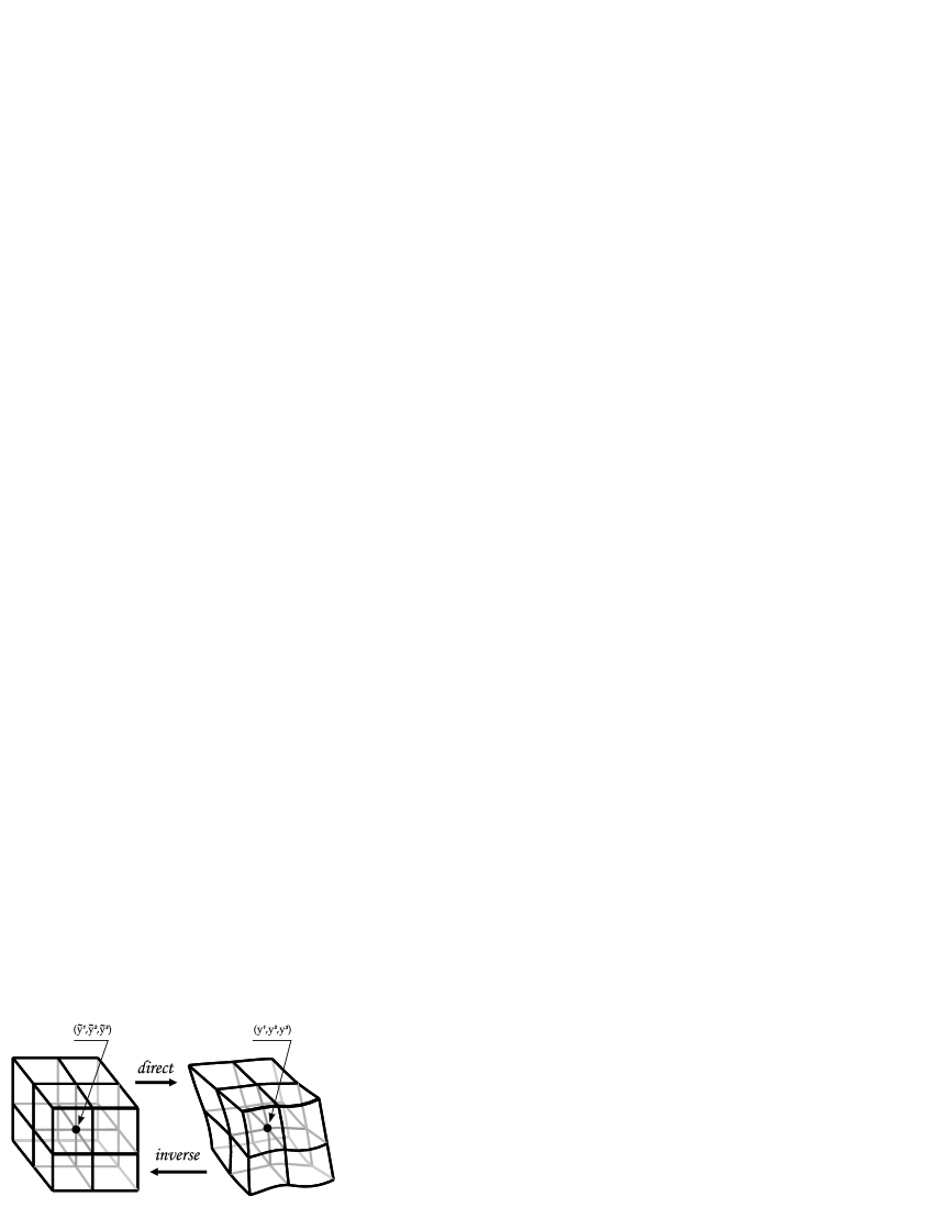
Figure 1:  Schematic presentation of the direct and inverse transformations on the deformation map. A point is transformed

The partial derivatives of the mapping functions (1) define two Jacobi matrices $\tilde{S}^{i}_{j}=\partial y^{i}/\partial\tilde{y}^{j}$ and $\tilde{T}^{i}_{j}=\partial\tilde{y}^{i}/\partial\tilde{y}^{j}$. The non-linear deformation tensor can be defined using one of them as pesented below:

$$\hskip-20.00003ptG_{ij}=\sum^{3}_{r=1}\sum^{3}_{s=1}g_{rs}(\tilde{y}^{1},\tilde{y}^{2},\tilde{y}^{3})\,\tilde{T}^{r}_{i}\,\tilde{T}^{s}_{j},$$ (2)

where $g_{rs}$ is the metric tensor arising through the useage of curvilinear coordinates S. F. Lyuksyutov, R. A. Sharipov , M. Heil, A. B. Hu . In Cartesian coordinates $g_{rs}$ is presented by the unit matrix; $\tilde{T}^{r}_{i}$, and $\tilde{T}^{s}_{j}$ are two Jacobi marices.

The tensor (2) is a quantitative measure of the deformation at given point of curvilinear coordinate system. Should a continuous medium be represented as a collection of infinetisemal cubes, then the tensor $G_{ij}$ completely describes how the edges and angles of these cubes contract, elongate and distort (as presented in Figure 1). Differentiating the formula (2)we arrive at the following evolution differential equation for the tensor $G_{ij}$:

$$\frac{\partial G_{ij}}{\partial t} +\sum^{3}_{r=1}v^{r}\,\nabla_{\!r}G_{ij}=$$ (3)

$$-\sum^{3}_{r=1}\nabla_{\!i}v^{r}\,G_{rj}-\sum^{3}_{r=1}G_{ir}\,\nabla_{\!j}v^{r}.$$

In order to describe plastic media, we separate the general deformation tensor into two tensors: $\hat{G}$, and $\check{G}$ are two parts of plastic deformation tensor of; $\hat{G}_{kq}$ is the tensor of elastic deformation:

$$\hskip-20.00003ptG_{ij}=\sum^{3}_{k=1}\sum^{3}_{q=1}\check{G}^{\,k}_{i}\,\hat{G}_{kq}\,\check{G}^{\,q}_{j}.$$ (4)

The choice of representing the plastic deformation tensor in two parts (instead of one as for elastic tensor) is related to the symmetry of the general tensor. The separation is the major step for the following consideration. The plastic deformation occurs in plastic materials that include pitch-like dense sticky liquids, solid amorphous materials, e. g. glasses, and polymers. These materials resist to the plastic deformation like solids and can flow like liquids. Unlike metals, where plastic deformation produces dislocations resulting in disorder of the crystalline grid, in our consideration, the plastic deformation does not change the material stucture.

The separation produces separate evolution equations for its plastic and elastic parts. The evolution equation of the plastic deformation $\check{G}$ can be presented as:

$$\frac{\partial\check{G}^{\,k}_{i}}{\partial t} +\sum^{3}_{r=1}v^{r}\,\nabla_{\!r}\check{G}^{\,k}_{i}=\sum^{3}_{r=1}\check{G}^{\,r}_{i}\,\nabla_{\!r}v^{k}$$ (5)

$$-\sum^{3}_{r=1}\nabla_{\!i}v^{r}\,\check{G}^{\,k}_{r}-\sum^{3}_{r=1}\theta^{\,k}_{r}\,\check{G}^{\,r}_{i}.$$

Here, as in equation (3) $v^{r}$ is the velocity of medium; $\nabla$ is the spatial derivative; $\theta$ is the physical parameter of continuous medium associated with the relaxation rate of elastic deformation into plastic.

Although the tensor $\theta^{\,k}_{r}$ is not symmetric, it can be obtained from the symmetric tensor $\theta_{ij}$ through the standard procedure of index raising. Using equations (3), (4), (5) we derive the evolution equation of elastic deformation. The evolution of elastic deformation is an important factor in determining the stress of a medium.

$$\hskip-20.00003pt\begin{gathered}\frac{\partial\hat{G}_{kq}}{\partial t}+\sum^{3}_{r=1}v^{r}\,\nabla_{\!r}\hat{G}_{kq}=-\sum^{3}_{r=1}\nabla_{\!k}v^{r}\,\hat{G}_{rq}\\ -\sum^{3}_{r=1}\hat{G}_{kr}\,\nabla_{\!q}v^{r}+\sum^{3}_{r=1}\theta^{\,r}_{k}\,\hat{G}_{rq}+\sum^{3}_{r=1}\hat{G}_{kr}\,\theta^{\,r}_{q}.\end{gathered}$$ (6)

Equations (5) and (6) must be complemented by three balance equations (three conservation laws for the flows of mass, momentum , and energy). The first is the mass balance equation:

$$\hskip-20.00003pt\frac{\partial\rho}{\partial t}+\sum^{3}_{k=1}\nabla_{\!k}(\,\rho\,v^{k})=0.$$ (7)

where $\rho$ is the density; $v^{k}$ is the velocity tensor. The next two equations are the momentum, and the energy balance equations:

$$\hskip-20.00003pt\frac{\partial(\,\rho\,v^{i})}{\partial t}+\sum^{3}_{k=1}\nabla_{\!k}\Pi^{ik}=f^{i},$$ (8)

$$\hskip-20.00003pt\frac{\partial}{\partial t}\!\left(\frac{\rho\,|\mathbf{v}|^{2}}{2}+\rho\,\varepsilon\right)+\sum^{3}_{k=1}\nabla_{\!k}w^{k}=e.$$ (9)

Here $f^{i}$ is the density of external forces acting on the medium, $e$ is the power of the forces; $v^{1}$, $v^{2}$, $v^{3}$ are the components of velocity vector $\mathbf{v}$; $\varepsilon$ is the specific inner thermal energy; $\Pi^{ik}$ and $w^{k}$ are the momentum, and energy flows determined by the following formulae:

$$\Pi^{ik}=\rho\,v^{i}\,v^{k}-\sigma^{ik}-\sum^{3}_{j=1}\sum^{3}_{q=1}\eta^{ikjq}\,v_{jq},$$

$$\begin{aligned} w^{k}&=\frac{\rho\,|\mathbf{v}|^{2}}{2}\,v^{k}+\rho\,\varepsilon\,v^{k}-\sum^{3}_{i=1}v_{i}\,\sigma^{ik}\\ &-\sum^{3}_{i=1}\sum^{3}_{j=1}\sum^{3}_{q=1}v_{i}\,\eta^{ikjq}\,v_{jq}-\sum^{3}_{i=1}\nabla_{\!i}T\,\varkappa^{ik},\end{aligned}$$

where $\sigma^{ik}$ is the stress tensor; $\eta^{ikjq}$ is the viscosity tensor; $\varkappa^{ik}$ is the heat conductivity tensor and $v_{jq}$ is the tensor of velocity gradients:

$$v_{ij}=\frac{\nabla_{\!i}v_{j}+\nabla_{\!j}v_{i}}{2}.$$

The parameter $\theta$ has the units of inverse time: $(sec^{-1})$, and determines the stress relaxation rate. The external forces produce stress and elastic deformation as a responce to this stress. In solely elastic material the responce is constant for constant deformation, and the parameter $\theta$ is zero. In plastic materials $\theta$ is non-zero and the exponential reduction of elastic response is observed. For constant general deformation $G$, the elastic component $\hat{G}$ in (4) decreases, while the plastic part $\check{G}$ increases. This scenario is presented in Figure 2.

Figure 2:  Conceptual presentation of parameter $\theta$. Elastic deformation produces stress relaxation resulting in plastic deformation through the conservation laws.

Further analysis of this model indicates that for materials in which the plastic deformation does not change the structure and produces no stress, it can excluded from consideration. This can be formulated through the ”‘forgetting principle”’. Suppose the medium evolves from an initial state at time $t=0$, to the intermediate state, at $t=t_{0}$, and then continues evolution for $t>t_{0}$. The principle asserts that if the intermediate state total deformation of medium was solely plastic, then the medium evolution occurs without memory of the intermediate state.

Equations (5)-(9) form a complete set describing the evolution of plastic medium in the frames of this model. They are used to describe the thermodynamics of plastic deformations. The specific internal thermal energy of the material depends on the entropy and on the elastic deformation. The differential of the energy can be written as:

$$\hskip-20.00003ptd\varepsilon=T\,ds-\sum^{3}_{i=1}\sum^{3}_{j=1}\frac{\bar{\sigma}^{ij}\,d\hat{G}_{ij}}{2\,\rho}$$ (10)

Here, $\bar{\sigma}^{ij}$ is an auxiliary tensor related to the stress tensor through the following formula:

$$\hskip-20.00003pt\sigma^{ij}=\sum^{3}_{r=1}\hat{G}^{\,i}_{r}\,\bar{\sigma}^{rj}.$$ (11)

Using equations (10), and (11) the time derivative of $\varepsilon$ and its gradient can be found. Substituting them into equation (9) and using the equations (5)-(8), we obtain the equation for specific entropy S. F. Lyuksyutov, R. A. Sharipov :

$$\hskip-20.00003pt\begin{gathered}\frac{\partial(\,\rho\,s)}{\partial t}+\sum^{3}_{k=1}\nabla_{\!k}\!\left(\rho\,s\,v^{k}-\smash{\sum^{3}_{i=1}}\frac{\nabla_{\!i}T\,\varkappa^{ik}}{T}\right)\\ =\sum^{3}_{i=1}\sum^{3}_{j=1}\frac{\sigma^{ij}\,\theta_{ij}}{T}+\sum^{3}_{i=1}\sum^{3}_{k=1}\frac{\nabla_{\!i}T\,\varkappa^{ik}\,\nabla_{\!k}T}{T^{2}}\\ +\sum^{3}_{i=1}\sum^{3}_{k=1}\sum^{3}_{j=1}\sum^{3}_{q=1}\frac{v_{ik}\,\eta^{ikjq}\,v_{jq}}{T}\end{gathered}$$ (12)

The three terms in the right hand side of equation (12) describe three different mechanisms of entropy production: plasticity, heat transfer, and viscosity. Second and third terms of (12) are typical for the visco-elastic solids. The term

$$\sum^{3}_{i=1}\sum^{3}_{j=1}\frac{\sigma^{ij}\,\theta_{ij}}{T}$$ (13)

responsible for plasticity is new one. It is non-zero indicating the growth of entropy on the way to equilibrium. Elastic deformation produces stress leading to plastic deformation, which in turn, results in additional entropy production as shown in (12).

Once introduced, the material parameter $\theta$ should be measured experimentally. The parameter can be found using calorimetric measuremens, as can be seen from the temperature dependence of the term (13). Alternatively, this parameter can be measured through the static bending of a polymer, or dynamic flow of the material. These two possible approaches for $\theta$ measurements are presented in Figure 3 below.

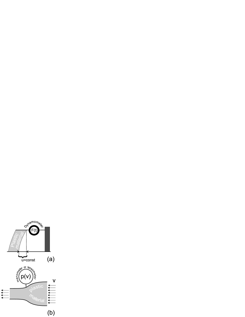
Figure 3:  (a)Static configuration of $\theta$ mesurement. A polymer sample of rectangular shape is subjected to shear bending through the application of lateral force $\mathbf{F}(t)$. The parameter $\theta$ can be determined by keeping $u=\operatorname{const}$ and measuring the force $\mathbf{F}$ as a function of time; (b)Dynamic configuration is comprised of the polymer pumped through the inverse nozzle. The pressure $p(v)$ on the walls of nozzle is measured as a function of velocity of incoming plastic flow, from which the components of tensor $\theta$ can be calculated.

In summary, we have suggested an approach for the separation of plastic deformation within general nonlinear tensor deformation. This separation allows for a robust description of the material’s plasticity using the relaxation rate introduced through the parameter $\theta$. This approach can be also used to describe experimental data of polymer deformation on nanoscale.

The authors acknowledge the support from National Research Council grant through the COBASE program. The authors wish to thank R. R. Mallik for the useful comments.

References

- E. L. Geist, D. J. Andrews [2000] E. L. Geist, D. J. Andrews, Journ. Geoph. Res., 105, 25543 (2000).
- S. J. Fiedor, J. M. Ottino [2003] S. J. Fiedor, J. M. Ottino, Phys. Rev. Lett. 91, 244301 (2003)
- P. G. de Genes [1990] P. G. de Genes, Introduction to Polymer Dynamics (Cambridge Univ. Press, Cambridge 1990)
- J. P. Hirth, J. Lothe [1968] J. P. Hirth, J. Lothe, Theory of Dislocations (McGraw Hill, New York,1968)
- [5] M. L. Falk, J. S. Langer, Phys. Rev. E 57, 7192 (1998).
- [6] A. E. Lobovsky, J. S. Langer, Phys. Rev. E 58, 1568 (1998).
- [7] D. R. Heine, G. S. Grest, E. B. Webb, Phys. Rev. E 68, 061603 (2003)
- [8] M. Akai-Kasaya, K. Shimizu, Y. Watanabe, A. Saito, M. Aono, Y. Kuwahara, Phys. Rev. Lett. 91, 255501 (2003)
- [9] S. F. Lyuksyutov, R. A. Vaia, P. B. Paramonov, S. Juhl, L. Waterhouse, R. M. Ralich, G. Sigalov, E. Sancaktar, Nature Materials, 2, 468 (2003)
- [10] S. F. Lyuksyutov, P. B. Paramonov, S. Juhl, R. A. Vaia, Appl. Phys. Lett. 83, 4405 (2003)
- [11] S. F. Lyuksyutov, R. A. Sharipov, G. Sigalov, and P. B. Paramonov, Cond-mat/0408247; http://www.arxiv.org/abs/cond-mat/0408247
- [12] E. Schaffer, T. Thurn-Albrecht, T. Russel, and U. Steiner, Nature 403, 874 (2000)
- [13] M. D. Morariu, N. A. Voicu, E. Schaeffer, Z. Lin, T. P. Russell, and U. Steiner, Nature Materials 2, 48 (2003)
- [14] P. Vettiger, M. Despont, U. Drechsler, U. Durig, W. Haberle, M. I. Lutwyche, H. E. Rothuizen, R. Stutz, R. Widmer, G. K. Binning, IBM J. Res. Develop. 44, 323 (2000)
- [15] H. J. Mamin, D. Rugar, Appl. Phys. Lett. 61, 1003 (1992)
- [16] A. A. Meyerhoff, I. Taner, A. E. L. Morris, W. B. Agocs, M. Kamen-Kaye, M. I. Bhat, N. Ch. Smoot, D. R. Choi, D. M. Hull, Surge Tectonics: A New Hypothesis of Global Geodynamics (Kluwer Academic Publishers, Dordrecht, 1996)
- [17] S. F. Lyuksyutov, R. A. Sharipov, Cond-mat/0304190; http://www.arxiv.org/abs/cond-mat/0304190
- [18] M. Heil, Nonlinear Elasticity and Computational Solid Mechanics, on-line lectures http://www.maths.man.ac.uk/~mheil/Lectures/NLElasticity/NLElasticity.html