Quantum phase transition in an atomic Bose gas near a Feshbach resonance

Abstract

We study the quantum phase transition in an atomic Bose gas near a Feshbach resonance in terms of the renormalization group. This quantum phase transition is characterized by an Ising order parameter. We show that in the low temperature regime where the quantum fluctuations dominate the low-energy physics this phase transition is of first order because of the coupling between the Ising order parameter and the Goldstone mode existing in the bosonic superfluid. However, when the thermal fluctuations become important, the phase transition turns into the second order one, which belongs to the three-dimensional Ising universality class. We also calculate the damping rate of the collective mode in the phase with only a molecular Bose-Einstein condensate near the second-order transition line, which can serve as an experimental signature of the second-order transition.

I Introduction

Trapped dilute cold atomic gases are one of the most exciting fields in condensed matter physics.A ; D An important recent development in this area is the application of Feshbach resonances. A Feshbach resonance in the scattering amplitude of two atoms occurs when the total energy of the atoms is close to the energy of a molecular state that is weakly coupled to the atomic continuum. Especially, the energy difference between the molecular state and the two-atom continuum, known as the detuning $\delta$, can be experimentally tuned by means of a magnetic field. Therefore, by sweeping the magnetic field from positive to negative detuning through the Feshbach resonance, it is actually possible to form molecules in the atomic gas.RTB ; SPH ; XMA In fact, recently, it has been possible to create a Bose-Einstein condensate (BEC) of molecules in an atomic Fermi gas with a Feshbach resonance.JBA ; GRJ ; ZSS This offers the opportunity for observing a Bardeen-Cooper-Schrieffer (BCS) transition in a dilute Fermi gas.

In the present paper, we study an analogous situation by varying $\delta$ in an atomic Bose gas with a Feshbach resonance. Two recent worksRPW ; RDS have shown that by varying $\delta$ there is a true quantum phase transition (QPT) in an atomic Bose gas, in contrast to the case of an atomic Fermi gas where a smooth BEC-BCS crossover exists as one changes $\delta$. An argument to understand this has been given in Ref. RDS, . We recapitulate it in the following to fix our notation. The effective Lagrangian describing a dilute atomic gas with a Feshbach resonance can be written as

$$L = \Psi_{a}^{\dagger}\!\left(\partial_{\tau}-\frac{\nabla^{2}}{2m}-\mu\right)\!\Psi_{a}+\Psi_{m}^{\dagger}\!\left(\partial_{\tau}-\frac{\nabla^{2}}{2M}-\tilde{\mu}\right)\!\Psi_{m}$$ (1)

$$+g_{0}\left(\Psi^{\dagger}_{m}\Psi_{a}\Psi_{a}+{\mathrm{H}.c.}\right)+u_{3}\Psi^{\dagger}_{m}\Psi_{a}^{\dagger}\Psi_{a}\Psi_{m}$$

$$+\frac{u_{1}}{2}\Psi^{\dagger}_{a}\Psi_{a}^{\dagger}\Psi_{a}\Psi_{a}+\frac{u_{2}}{2}\Psi^{\dagger}_{m}\Psi_{m}^{\dagger}\Psi_{m}\Psi_{m}\ ,$$

with $\tilde{\mu}=2\mu-\delta$. Here $\Psi_{a}$ and $\Psi_{m}$ are the annihilation operators of atoms and molecules, respectively. $m$ and $M$ are the mass of the atom and that of the molecule, respectively. In the path integral formula, $\Psi_{m}$ is an ordinary number. On the other hand, $\Psi_{a}$ is an ordinary number for the atomic Bose gas, while it is a Grassmann number for the atomic Fermi gas. (For the atomic Fermi gas, $\Psi_{a}$ contains the indices for hyperfine spins and should be understood as a spinor.) The Lagrangian $L$ [Eq. (1)] has a U($1$) symmetry. That is, it is invariant against the U($1$) transformation

$$\Psi_{a}\rightarrow e^{i\alpha}\Psi_{a}\ ,~{}~{}\Psi_{m}\rightarrow e^{2i\alpha}\Phi_{m}\ .$$ (2)

For an atomic Bose gas, due to the $g_{0}$ term, a nonzero value of $\langle\Psi_{a}\rangle$ (atomic BEC) must lead to a nonzero value of $\langle\Psi_{m}\rangle$ (molecular BEC). However, the reverse is not true. That is, it is possible for the gas to contain only a molecular BEC. In the case with both atomic BEC and molecular BEC, the U($1$) symmetry of $L$ is completely broken. But for the case with only molecular BEC there is a residual Z₂ symmetry. That is, the effective Lagrangian in this case is invariant against the Z₂ transformation: $\Psi_{a}\rightarrow-\Psi_{a}$ and $\Psi_{m}\rightarrow\Psi_{m}$. The above analysis indicates that at low temperature the atomic Bose gas with a Feshbach resonance has two thermodynamically distinct phases: the “atomic superfluid” (ASF) phase with both atomic BEC and molecular BEC, and the “molecular superfluid” (MSF) phase with molecular BEC only. For an atomic Fermi gas, due to the $g_{0}$ term, a nonzero value of $\langle\Psi_{a}\Psi_{a}\rangle$ must be accompanied with a nonvanishing value of $\langle\Psi_{m}\rangle$ and vice versa. Therefore, the BCS region has the same symmetry as the BEC region, and only a crossover occurs.

Based on the above observation, the MSF phase is distinct from the ASF phase by a Z₂ symmetry. Thus, the phase transition between the two phases is characterized by an Ising (Z₂) order parameter. Naively, one may expect that this QPT is of second order and belongs to the four-dimensional ($4d$) Ising universality class at zero temperature and the three-dimensional ($3d$) Ising universality class at finite temperature. However, there is a gapless excitation in the MSF phase, which is the Goldstone mode associated with the molecular BEC. An additional gapless excitation may result in severe IR divergences and modify the critical behavior. Therefore, a proper theory describing the QPT should consist of the Ising order parameter as well as the Goldstone mode. A renormalization group (RG) analysis indicates that the coupling between the Ising order parameter and the Goldstone mode will drive the zero-temperature phase transition to become weakly first orderFB through the Colemann-Weinberg mechanism.CW The question in which we are interested here is the nature of this phase transition at finite temperature. We study this problem in terms of the RG. Our main results are shown in Fig. 1, which are valid at the temperature much lower than the amplitude fluctuations in the molecular BEC. At low temperature where the quantum fluctuations dominate the low-energy physics, the phase transition between the MSF and ASF phases is of weakly first order. When the thermal fluctuations become important, the effects of the coupling between the Ising order parameter and the Goldstone mode are suppressed and the transition becomes a second-order one belonging to the $3d$ Ising universality class. Thus, a tricritical point must exist on the phase boundary to separate these two kinds of phase transition.

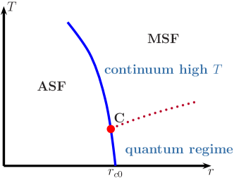
Figure 1: The schematic phase diagram of the dilute Bose gas with single Feshbach resonance near the transition line between the ASF and MSF phases below $T_{c}(\delta)$, where $T_{c}(\delta)$ represents the transition temperature between the normal Bose gas and the superfluid phase. The dotted line denotes the crossover from low temperature to high temperature regimes. The solid line is the phase boundary between the ASF and MSF phases. The point $C$ is a tricritical point. On the phase boundary, the portion below the point $C$ is of first order while the one above the point $C$ is of second order.

The rest of the paper is organized as follows: We write down the effective Lagrangian describing the QPT by symmetry argument and perform one-loop RG analysis in Sec. II. The solution of the scaling equations is presented in Sec. III. In Sec. IV, we calculate the damping rate of the collective excitation in the MSF phase near the second-order transition line. The last section is devoted to our conclusion.

II Landau theory and renormalization group analysis

II.1 Effective Lagrangian

We start with the “normal phase” for this QPT. The fundamental fields of the effective theory describing the QPT consist of the Ising order parameter $\phi$, which can be taken as the imaginary part of $\Psi_{a}$, and the phase of $\Psi_{m}$, $\theta$. Following Landau, the corresponding effective Lagrangian can be written down through symmetry consideration. The symmetries involved here are the Z₂ symmetry, a subgroup of the U($1$) symmetry [Eq. (2)], under which the $\phi$ and $\theta$ fields transform as

$$\phi\rightarrow-\phi\ ,~{}~{}\theta\rightarrow\theta+2\pi\ ,$$ (3)

and the U($1$) symmetry under which $\theta$ transforms as $\theta(x)\rightarrow\theta(x)+\alpha$ where $\alpha$ is an arbitrary constant. The most general local action consistent with the Z₂ and U($1$) symmetries is $I=I_{\phi}+I_{\theta}+I_{int}$ where

$$I_{\phi}=\!\!\int\!\!d\tau d^{3}x\left\{\frac{1}{2}\left[\left(\frac{1}{c_{0}}\partial_{\tau}\phi\right)^{2}\!\!+(\bm{\nabla}\phi)^{2}\right]\!\!+\frac{t_{0}}{2}\phi^{2}+\frac{u_{0}}{4!}\phi^{4}\!\right\},$$ (4)

with $u_{0}>0$,

$$I_{\theta}=\frac{\rho_{s}}{2M}\int\!\!d\tau d^{3}x\left[\!\left(\frac{1}{v_{0}}\partial_{\tau}\theta\right)^{2}+(\bm{\nabla}\theta)^{2}\right],$$ (5)

and

$$I_{int}=\int\!\!d\tau d^{3}x~{}i\lambda_{0}\partial_{\tau}\theta\phi^{2}\ .~{}~{}~{}~{}~{}~{}~{}$$ (6)

Here $t_{0}$ measures the (mean-field) distance from the transition point. ($t_{0}>0$ in the MSF phase while $t_{0}<0$ in the ASF phase.) $\rho_{s}$ is the ”bare” superfluid density and $c_{0}$ and $v_{0}$ are ”bare” velocities for the order parameter $\phi$ and the Goldstone boson $\theta$, respectively. In Eq. (6), only the most relevant (near the transition point) coupling between the Goldstone mode and the order parameter is kept. The factor $i$ in Eq. (6) is dictated by the charge conjugation symmetry of the original Lagrangian $L$ [Eq. (1)]. It requires that $L\rightarrow L^{\dagger}$ when $\Psi_{a}\rightarrow\Psi_{a}^{\dagger}$ and $\Psi_{m}\rightarrow\Psi_{m}^{\dagger}$, which leads to $I\rightarrow I^{\dagger}$ when $\phi\rightarrow-\phi$ and $\theta\rightarrow-\theta$. The natural cutoff of this action is provided by the gap of amplitude fluctuations in the molecular BEC. A similar action has appeared in other context.FB

The action (4) — (6) can also be derived from the Lagrangian $L$ [Eq. (1)] by considering the fluctuations around its mean-field solution in the MSF phase. By integrating out the sectors with finite gaps at the transition point, i.e. the real part of $\Psi_{a}$ and the amplitude of $\Psi_{m}$, in terms of the perturbation theory in $u_{1}$, $u_{2}$, $u_{3}$, and $g_{0}/\sqrt{n}$, to the leading order, one may obtain

$$c_{0}\approx\sqrt{\frac{g_{0}}{m}}\left(2n\right)^{1/4}\ ,$$

$$t_{0}=m(\delta_{0}-\delta)\ ,$$

$$u_{0}\approx 12mu_{1}\!\left[1-\frac{1}{u_{1}u_{2}}\left(u_{3}+\sqrt{\frac{2}{n}}~{}g_{0}\right)^{2}\right],$$

$$\rho_{s}\approx\frac{n}{2}\ ,$$

$$v_{0}\approx\sqrt{\frac{u_{2}n}{2M}}\ ,$$

$$\lambda_{0}\approx\frac{m}{2}\left[1-\frac{2}{u_{2}}\left(u_{3}+\sqrt{\frac{2}{n}}~{}g_{0}\right)\right],$$ (7)

near the transition point. (Here we take the real part of $\Psi_{a}$ as the gapped sector at the transition point. This amounts to assuming $g_{0}>0$.) In Eq. (7), $n$ is the total particle density and $\delta_{0}$ denotes the magnetic field detuning at which the zero-temperature quantum phase transition occurs at the mean-field level, which is given by $\delta_{0}\approx\left(u_{3}-\frac{u_{2}}{2}\right)n-2^{3/2}g_{0}n^{1/2}$. (This value of $\delta_{0}$ has already been given by Ref. RPW, .) From Eq. (7), it is obvious that the value of $u_{0}$ may become negative in some parameter regime. For $u_{0}<0$, one should include the terms with higher powers of $\phi$ like $\phi^{6}$ in $I_{\phi}$ to make it stable, and the QPT between the MSF and ASF phases will be of first order,KH even in the absence of the coupling to the Goldstone mode $\theta$. In this case, it is of little interest because the correlation length is always finite and thus there are no universal behaviors for physical quantities at both zero and finite temperatures. Therefore, in the following, we shall concentrated on the parameter regime which gives rise to a positive value of $u_{0}$. From Eq. (7), this corresponds to $(u_{3}+\sqrt{2/n}~{}g_{0})^{2}<u_{1}u_{2}$.

At $T=0$, $I_{\phi}$ with $u_{0}>0$ describes the $4d$ Ising universality class. It exhibits a Gaussian behavior with logarithmic corrections due to the presence of the marginally irrelevant coupling $u_{0}$. Therefore, we may consider the RG transformation

$$\tau\rightarrow\tau/s\ ,~{}~{}\bm{x}\rightarrow\bm{x}/s\ ,$$

$$\phi\rightarrow s\phi\ ,~{}~{}\theta\rightarrow s\theta\ ,$$ (8)

while $c_{0}$, $v_{0}$, $\rho_{s}$, and $M$ remain invariant. Here $s>1$ is the rescaling factor. Then, the action $I_{\phi}+I_{\theta}+I_{int}$ with $u_{0}=0=\lambda_{0}$ is invariant under the RG transformation [Eq. (8)]. It is straightforward to see that the coupling constants $u_{0}$ and $\lambda_{0}$ are marginal at the tree level with respect to the Gaussian fixed point under the RG transformation [Eq. (8)]. Within the weak-coupling region, one-loop RG equations are needed to determine their roles on the low-energy physics.

II.2 One-loop RG equations

To compute the one-loop RG equations, we employ the momentum-shell RG. Before integrating out the fast modes, we make a change on the variables:

$$\bm{x}\rightarrow\Lambda^{-1}\bm{x}\ ,~{}~{}\tau\rightarrow\Lambda^{-1}c_{0}^{-1}\tau\ ,~{}~{}v=v_{0}/c_{0}\ ,$$

$$\phi\rightarrow\Lambda c_{0}^{1/2}\phi\ ,~{}~{}\theta\rightarrow\Lambda\!\left(\frac{c_{0}M}{\rho_{s}}\right)^{1/2}\!\theta\ ,$$

$$r=\Lambda^{-2}t_{0}\ ,~{}~{}u=c_{0}u_{0}\ ,~{}~{}\beta=\frac{\Lambda c_{0}}{T}\ ,$$

$$\lambda=\left(\frac{c_{0}^{3}M}{\rho_{s}}\right)^{1/2}\!\lambda_{0}\ ,$$

where $\Lambda$ is an UV cutoff in momenta and $T$ is the temperature. Then, $v$, $r$, $u$, $\lambda$, and $\beta$ become dimensionless parameters and our working action is written as $I=\int^{\beta}_{0}\!\!d\tau\!\int\!\!d^{3}x~{}{\mathcal{L}}$ where

$${\mathcal{L}} = \frac{1}{2}\left[(\partial_{\tau}\phi)^{2}+(\bm{\nabla}\phi)^{2}\right]+\frac{1}{2}~{}r\phi^{2}+\frac{1}{4!}~{}u\phi^{4}$$ (9)

$$+\frac{1}{2}\left[\left(\frac{1}{v}~{}\partial_{\tau}\theta\right)^{2}+(\bm{\nabla}\theta)^{2}\right]+i\lambda\partial_{\tau}\theta\phi^{2}\ .~{}~{}$$

By integrating out the fast modes, i.e. those modes with momenta within the momentum shell $e^{-l}<|\bm{k}|<1$ where $e^{-l}$ is the scaling factor, we obtain the one-loop RG equations:

$$\frac{dt_{l}}{dl}=t_{l}\ ,$$ (10)

$$\frac{dv_{l}}{dl}=-\frac{K_{l}v_{l}}{4(1+r_{l})^{3/2}}~{}f_{2}(\sqrt{1+r_{l}}/t_{l})\ ,$$ (11)

$$\frac{dr_{l}}{dl}=2r_{l}+\frac{U_{l}t_{l}}{4(1+r_{l})}f_{1}(\sqrt{1+r_{l}}/t_{l})$$

$$~{}~{}~{}~{}~{}~{}~{}~{}+\frac{2K_{l}}{t_{l}}~{}g_{1}(\sqrt{1+r_{l}}/t_{l},v_{l}/t_{l})\ ,$$ (12)

$$\frac{dK_{l}}{dl}=-\frac{K_{l}}{4}(U_{l}+2K_{l})\frac{f_{2}(\sqrt{1+r_{l}}/t_{l})}{(1+r_{l})^{3/2}}$$

$$~{}~{}~{}~{}~{}~{}~{}~{}-\frac{2K_{l}^{2}}{\sqrt{1+r_{l}}(1+r_{l}-v_{l}^{2})}~{}g_{2}(\sqrt{1+r_{l}}/t_{l},v_{l}/t_{l})$$

$$~{}~{}~{}~{}~{}~{}~{}~{}+\frac{4K_{l}^{2}t_{l}}{(1+r_{l}-v_{l})^{2}}~{}f_{1}(v_{l}/t_{l})\ ,$$ (13)

$$\frac{dU_{l}}{dl}=-24K_{l}^{2}\frac{\sqrt{1+r_{l}}}{(1+r_{l}-v_{l}^{2})^{2}}~{}g_{3}(\sqrt{1+r_{l}}/t_{l},v_{l}/t_{l})$$

$$~{}~{}~{}~{}~{}~{}~{}~{}+24K_{l}^{2}\frac{v_{l}}{(1+r_{l}-v_{l}^{2})^{2}}~{}g_{4}(\sqrt{1+r_{l}}/t_{l},v_{l}/t_{l})$$

$$~{}~{}~{}~{}~{}~{}~{}~{}-\frac{6K_{l}U_{l}}{\sqrt{1+r_{l}}(1+r_{l}-v_{l}^{2})}~{}g_{2}(\sqrt{1+r_{l}}/t_{l},v_{l}/t_{l})$$

$$~{}~{}~{}~{}~{}~{}~{}~{}+\frac{12K_{l}U_{l}t_{l}}{(1+r_{l}-v_{l}^{2})^{2}}~{}f_{1}(v_{l}/t_{l})$$

$$~{}~{}~{}~{}~{}~{}~{}~{}-\frac{3U_{l}^{2}}{8(1+r_{l})^{3/2}}~{}f_{2}(\sqrt{1+r_{l}}/t_{l})\ ,$$ (14)

where $t=1/\beta$, $K=(\lambda v)^{2}/(2\pi^{2})$, $U=u/(2\pi^{2})$ and

$$f_{1}(x)=x\coth{\!\left(\frac{x}{2}\right)}\ ,$$

$$f_{2}(x)=\coth{\!\left(\frac{x}{2}\right)}+\frac{x}{2}\sinh^{-2}{\!\left(\frac{x}{2}\right)}\ ,$$

$$g_{1}(x,y)=\frac{f_{1}(x)-f_{1}(y)}{x^{2}-y^{2}}\ ,$$

$$g_{2}(x,y)=\frac{x^{2}+y^{2}}{x^{2}-y^{2}}~{}\coth{\!\left(\frac{x}{2}\right)}+\frac{x}{2}\sinh^{-2}{\!\left(\frac{x}{2}\right)}\ ,$$

$$g_{3}(x,y)=\frac{x^{2}+3y^{2}}{x^{2}-y^{2}}~{}\coth{\!\left(\frac{x}{2}\right)}+\frac{x}{2}\sinh^{-2}{\!\left(\frac{x}{2}\right)}\ ,$$

$$g_{4}(x,y)=\frac{3x^{2}+y^{2}}{x^{2}-y^{2}}~{}\coth{\!\left(\frac{y}{2}\right)}-\frac{y}{2}\sinh^{-2}{\!\left(\frac{y}{2}\right)}\ .$$

Here the rescaled quantities have explicit $l$ dependence indicated, e.g. $t_{l}$, while quantities without $l$ dependence (e.g. $T$) refer to physical quantities.

Since $K>0$, we always have $dv_{l}/dl<0$ from Eq. (11), and thus $v_{l}$ will flow to zero. Therefore, we may set $v_{l}=0$ in Eqs. (12) —(14), yielding

$$\frac{dr_{l}}{dl}=2r_{l}-\frac{4K_{l}t_{l}}{1+r_{l}}+\frac{(U_{l}+8K_{l})t_{l}}{4(1+r_{l})}f_{1}\!\!\left(\frac{\sqrt{1+r_{l}}}{t_{l}}\right),~{}~{}~{}~{}~{}~{}$$ (15)

$$\frac{dK_{l}}{dl}=\frac{8K_{l}^{2}t_{l}}{(1+r_{l})^{2}}-\frac{K_{l}}{4}\frac{U_{l}+10K_{l}}{(1+r_{l})^{3/2}}f_{2}\!\!\left(\frac{\sqrt{1+r_{l}}}{t_{l}}\right),$$ (16)

$$\frac{dU_{l}}{dl}=\frac{24K_{l}U_{l}t_{l}}{(1+r_{l})^{2}}-\frac{3}{8}\frac{(U_{l}+8K_{l})^{2}}{(1+r_{l})^{3/2}}f_{2}\!\!\left(\frac{\sqrt{1+r_{l}}}{t_{l}}\right).$$ (17)

The solution of Eq. (10) is simply given by

$$t_{l}=te^{l}\ .$$ (18)

In the next section, we shall solve Eqs. (15) — (17) approximately by neglecting the possible logarithmic corrections.

III Solution of scaling equations

Scaling stops when $|r_{l}|\sim 1$. One must distinguish two regimes: $t_{l}\ll 1$ and $t_{l}\gg 1$. The former corresponds to the quantum ($T=0$) regime where the quantum fluctuations dominate the low-energy physics. Otherwise, it is the continuum high $T$ regime where the thermal fluctuations become important.

III.1 Quantum regime

In the quantum regime, the nonlinear dependence of the RG functions (those terms appearing at the R.H.S. of Eqs. (15) — (17)) on $r_{l}$ will not be important. Thus, we shall consider the limiting equations, valid for $r,K,U\ll 1$

$$\frac{dr_{l}}{dl}=2r_{l}-4K_{l}t_{l}+\!\!\left(\frac{U_{l}}{4}+2K_{l}\right)t_{l}f_{1}\!\!\left(\frac{1}{t_{l}}\right),$$ (19)

$$\frac{dK_{l}}{dl}=8K_{l}^{2}t_{l}-\frac{K_{l}}{4}(U_{l}+10K_{l})f_{2}\!\!\left(\frac{1}{t_{l}}\right),$$ (20)

$$\frac{dU_{l}}{dl}=24K_{l}(U_{l}+4K_{l})t_{l}-\!\frac{3}{8}(U_{l}+8K_{l})^{2}f_{2}\!\!\left(\frac{1}{t_{l}}\right).~{}~{}~{}~{}~{}~{}$$ (21)

To obtain the condition on $T$ for the occurrence of the quantum regime, one may set $t=0$ in Eqs. (19) — (21), yielding

$$\frac{dr_{l}}{dl}=2r_{l}+\frac{1}{6}{\mathcal{X}}_{l}+\frac{1}{12}U_{l}\ ,$$ (22)

$$\frac{d{\mathcal{X}}_{l}}{dl}=-\frac{3}{8}{\mathcal{X}}_{l}^{2}\ ,$$ (23)

$${\mathcal{X}}_{l}\frac{d{\mathcal{Y}}_{l}}{d{\mathcal{X}}_{l}}=\frac{1}{9}({\mathcal{Y}}_{l}-4)({\mathcal{Y}}_{l}-1)\ .$$ (24)

Here ${\mathcal{X}}_{l}=U_{l}+12K_{l}$ and ${\mathcal{Y}}_{l}=U_{l}/{\mathcal{X}}_{l}$. The solution of Eqs. (23) and (24) is written as

$${\mathcal{X}}_{l}=\frac{x_{0}}{1+3x_{0}l/8}\ ,$$

$$U_{l}=\frac{d_{0}{\mathcal{X}}_{l}^{1/3}-4}{d_{0}{\mathcal{X}}_{l}^{1/3}-1}~{}{\mathcal{X}}_{l}\ ,$$ (25)

where $x_{0}=U+12K$ and the value of $d_{0}$ is chosen such that $U_{l}=U$ when ${\mathcal{X}}_{l}=x_{0}$. (In fact, $d_{0}x_{0}^{1/3}=4+U/(4K)$. Therefore, $d_{0}\gg 1$ for $K,U\ll 1$.)

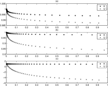
Figure 2: Typical solutions of Eqs. (22)—(24) with the initial conditions (a) $r=0.002$, $K=0.0003$, and $U=0.005$, (b) $r=0.002$, $K=0.003$, and $U=0.005$, and (c) $r=0.002$, $K=0.03$, and $U=0.005$. The $x$-axis is $r_{l}$ and the $y-axis$ is $K_{l}/K$ or $U_{l}/U$.

By solving Eqs. (22) — (24) numerically, we notice that the value of $K_{l}$ remains almost unchanged when $r_{l}\leq 1$, as shown in Fig. 2. However, the behavior of $U_{l}$ depends on the sign of the function $G(r,U,K)$, roughly given by

$$G(r,U,K)\approx\frac{16}{3x_{0}}\left[\!\left(1+\frac{U}{16K}\right)^{3}\!-1\right]\!-\ln{(1/r)}\ .$$ (26)

(Equation (26) is determined from Eq. (25) by requiring that $U_{l^{*}}=0$ or $d_{0}{\mathcal{X}}_{l^{*}}^{1/3}=4$ where $r_{l^{*}}=1$. The condition $r_{l^{*}}=1$ roughly gives rise to $2l^{*}\approx\ln{(1/r)}$.) (i) As $G(r,U,K)>0$, $U_{l}>0$ and its magnitude does not change much for $r_{l}\leq 1$, as shown in Fig. 2 (a) and (b). (ii) As $G(r,U,K)<0$, the value of $U_{l}$ becomes negative rapidly before $r_{l}=1$ as shown in Fig. 2 (c).

For given $K$ and $U$, we may increase the value of $r$ starting with $r=0$. In the beginning, $G(r,K,U)<0$ and $U$ becomes negative when scaling stops. Thus, a $\phi^{6}$ term must be included in the effective action. A mean-field theory in this case gives rise to $\langle\phi\rangle\neq 0$. This corresponds to the ASF phase. On the other hand, for sufficiently large $r$ such that $G(r,U,K)>0$, $U$ is still positive when scaling stops, and thus a mean-field theory gives rise to $\langle\phi\rangle=0$. This corresponds to the MSF phase. Consequently, there are two phases at zero temperature separated by a transition point, denoted by $r_{c0}$. The value of $r_{c0}$ can be estimated by requiring that $G(r_{c0},U,K)=0$. A negative value of $U$ is usually interpreted as a fluctuation-induced first-order phase transition.AZ Therefore, the QPT at $T=0$ is of first order. In the following, we shall focus on case (i), i.e. the Z₂ symmetric (MSF) phase.

In case (i), because the values of $K_{l}$ and $U_{l}$ do not change significantly when scaling stops, we may set $K_{l}={\mathcal{K}}>0$ and $U_{l}={\mathcal{U}}>0$ in Eq. (22) for simplicity, where ${\mathcal{K}}/K\approx 1$ and ${\mathcal{U}}/U\leq 1$. Within this approximation, the logarithmic corrections are neglected. (The approximation we use amounts to neglecting the $l$ dependence of ${\mathcal{X}}_{l}$. Inclusion of it will result in logarithmic corrections.) Setting $r_{l}=1$, solving for $l$, substituting the result into Eq. (18), and demanding $t_{l}\ll 1$, one may obtain the condition for the occurrence of the quantum regime in the MSF phase:

$$t\ll\left(\frac{r+A_{1}}{1+A_{1}}\right)^{1/2}\ ,$$ (27)

where $A_{1}={\mathcal{K}}+{\mathcal{U}}/8$.

In terms of Eq. (7), the crossover line between the quantum and continuum high $T$ regimes in the MSF phase, corresponding to $r>r_{c0}$, can be expressed by

$$\left(\frac{T}{c_{0}}\right)^{2}\approx t_{0}+\frac{c_{0}\Lambda^{2}}{2\pi^{2}}\left(u_{2}\lambda_{0}^{2}+\frac{u_{0}}{8}\right)\ ,$$ (28)

as shown in Fig. 1. Here the values of $c_{0}$, $t_{0}$, $\lambda_{0}$, and $u_{0}$ near the transition point is given by Eq. (7). In addition, the momentum UV cutoff $\Lambda$ can be estimated by $\Lambda\approx min\{2^{5/4}\sqrt{mg_{0}}~{}n^{1/4},\sqrt{u_{2}M/2}~{}n^{1/2}\}$, where the former and the latter arise from the gap of the real part of $\Psi_{a}$ and that of the amplitude fluctuations of $\Phi_{m}$, respectively. To obtain Eq. (28), we have neglected $1+A_{1}$ in Eq. (27) because $A_{1}\ll 1$. Further, ${\mathcal{K}}$ and ${\mathcal{U}}$ are replaced by $K$ and $U$, respectively.

Finally, we determine the correlation length in the quantum regime. To do so, we may set $K_{l}={\mathcal{K}}$ and $U_{l}={\mathcal{U}}$ in Eq. (19) and performing low-temperature expansion, yielding

$$\frac{dr_{l}}{dl}=2r_{l}+2A_{1}-4{\mathcal{K}}te^{l}\ .$$ (29)

The solution of Eq. (29) is written as

$$r_{l}=e^{2l}\left[r+A_{1}\left(1-e^{-2l}\right)-4{\mathcal{K}}t\left(1-e^{-l}\right)\right].$$ (30)

The correlation length is given by $\xi\sim e^{l^{*}}$ where $r_{l^{*}}=1$. From Eq. (30), one may obtain

$$\xi\sim(r+A_{1}-A_{2}t)^{-1/2}\ ,$$ (31)

with $A_{2}=4{\mathcal{K}}$. Therefore, $\xi$ is always finite for given $t$ satisfying the inequality (27), as expected for a first-order phase transition. To sum up, the phase transition between the MSF and ASF phases in the quantum (low temperature) regime is of weakly first-order.

III.2 Continuum high $T$ regime

In this regime, it is convenient to divide the scaling into two steps: $t_{l}\ll 1$ and $t_{l}\gg 1$. This introduces multiplicative errors of order unit coming from the imprecise treatment of the crossover regime $t_{l}\sim 1$. In the first step, we integrate over $l$ from $0$ to $\tilde{l}$, such that $t_{\tilde{l}}=1$. Next we consider the case $t_{l}\gg 1$. In this case, it is more convenient to define the coupling $V_{l}=t_{l}U_{l}$. We would like to show that the RG equations for $r_{l}$ and $V_{l}$ in the continuum high $T$ regime are identical to those for the $3d$ Ising model.

We start with Eqs. (15) and (17) and take $t_{l}\gg 1$. Using $f_{1}(0)=2$ and $f_{2}(x\rightarrow 0)\approx 4/x$, we obtain

$$\frac{dr_{l}}{dl}=2r_{l}+\frac{V_{l}}{2(1+r_{l})}\ ,$$ (32)

$$\frac{dV_{l}}{dl}=V_{l}-\frac{3V_{l}^{2}}{2(1+r_{l})^{2}}\ .$$ (33)

Equations (32) and (33) are identical to the one-loop RG equations for the $3d$ Ising model. Therefore, we conclude that the transition between the MSF and ASF phases in the continuum high $T$ regime is of second order and belongs to the $3d$ Ising universality class. Near the transition point, the solution of Eqs. (32) and (33) is given by

$$r_{l}-r^{*}\approx(\tilde{r}-r^{*})e^{l/\nu_{3}}\ ,~{}~{}V_{l}\approx V^{*}\ ,$$ (34)

where $\nu_{3}\approx 0.63$ is the correlation length exponent for the $3d$ Ising model and $\tilde{r}=r_{\tilde{l}}$, which are determined by the RG equations in the quantum regime. Here $r^{*}$ and $V^{*}$ are the fixed points of Eqs. (32) and (33), which within the $\epsilon$ expansion corresponds to the Wilson-Fisher fixed point, where $\epsilon=4-d$ and $d$ is the spatial dimensions. The exact values of $r^{*}$ and $V^{*}$ are nonuniversal, and the determination of them is beyond the present field-theoretical approach.

To determine $\tilde{r}$, we shall focus on the MSF phase. In this case, one may neglect the possible logarithmic corrections and set $K_{l}=\overline{{\mathcal{K}}}>0$ and $U_{l}=\overline{{\mathcal{U}}}>0$ where $\overline{{\mathcal{K}}}/K\approx 1$ and $\overline{{\mathcal{U}}}/U\leq 1$. (Note that both $\overline{{\mathcal{K}}}$ and $\overline{{\mathcal{U}}}$ may not be equal to ${\mathcal{K}}$ and ${\mathcal{U}}$.) Then, from Eq. (19), we obtain

$$\tilde{r}=\frac{r+B_{1}}{t^{2}}-\frac{B_{2}}{t}+C\ ,$$ (35)

where $B_{1}=\overline{{\mathcal{K}}}+\overline{{\mathcal{U}}}/8$, $B_{2}=4\overline{{\mathcal{K}}}$, and

$$C=3\overline{{\mathcal{K}}}-\frac{\overline{{\mathcal{U}}}}{8}+4B_{1}\int^{1}_{0}\!\!dy~{}y^{-3}n_{B}(y^{-1})\ ,$$

with $n_{B}(x)=(e^{x}-1)^{-1}$.

Scaling stops when $|r_{l^{*}}-r^{*}|=1$. The correlation length is given by $\xi\sim e^{\tilde{l}}e^{l^{*}}=t^{-1}e^{l^{*}}$. Equation (34) gives rise to

$$l^{*}\approx-\nu_{3}\ln{\!\left|\frac{r+B_{1}}{t^{2}}-\frac{B_{2}}{t}+B_{3}\right|}\ ,$$

where $B_{3}=C-r^{*}$ is a nonuniversal constant. As a result, we get

$$\xi\sim t^{-1}\left[\frac{|r-r_{c}(t)|}{t^{2}}\right]^{-\nu_{3}}\ ,$$ (36)

where $r_{c}(t)=-B_{1}+B_{2}t-B_{3}t^{2}$ denotes the transition point between the MSF and ASF phases for given temperature. Equation (36) is valid up to logarithmic corrections.

Finally, we consider the RG equation for $K_{l}$ in the continuum high $T$ regime, which can be written as

$$U_{l}\frac{dR_{l}}{dU_{l}}=\frac{4}{3}~{}R_{l}^{2}-\frac{1}{3}~{}R_{l}\ ,$$ (37)

where $R=K/U$. Solving Eq. (37) gives rise to

$$K_{l}\approx\frac{V^{*}}{4}~{}e^{-l}\ ,$$ (38)

near the transition line. When scaling stops, we may perform the perturbation theory in $K_{l}$ and $V_{l}$ as long as $V^{*},K_{l^{*}}=V^{*}/(4\xi t)\ll 1$. Within the spirit of the $\epsilon$ expansion, it is indeed the case because $V^{*}=O(\epsilon)$.

IV Damping rate of collective excitations in the MSF phase

The damping in the collective excitations of condensates will become much more severe near the second-order transition line due to the coupling to the critical fluctuations. Therefore, a measurement of the damping in the collective modes may serve as a signature of the second-order Ising transition between the MSF and ASF phases. In this section, we shall use the RG equations to calculate the damping rate of the collective mode in the MSF phase near the second-order transition line, arising from the coupling to the critical fluctuations. Since the identification of the Ising transition is established within the $\epsilon$ expansion, the following RG-improved perturbative calculation is supposed to be understood within such a context.

The full propagator of the $\theta$ field can be written as $D^{-1}(i\omega_{n},\bm{k})=D^{-1}_{0}(i\omega_{n},\bm{k})+\Sigma_{\theta}(i\omega_{n},\bm{k})$ where $\omega_{n}=2n\pi/\beta$, $\Sigma_{\theta}$ is the self-energy of the $\theta$ field, and

$$D_{0}(k)=\frac{1}{\omega_{n}^{2}/v^{2}+\bm{k}^{2}}\ ,$$

is the free propagator of the $\theta$ field. The spectrum is determined by

$$D^{-1}(i\omega_{n}\rightarrow\omega+i0^{+},\bm{k})=0\ ,$$

which gives rise to $\omega=\epsilon_{\bm{k}}-i\gamma_{\bm{k}}$ where $\gamma_{\bm{k}}$ denotes the damping rate and $\epsilon_{\bm{k}}$ is the dispersion relation of the collection mode. In the long wavelength limit, $\epsilon_{\bm{k}}=\overline{v}k$ where $k=|\bm{k}|$ and $\overline{v}$ is the dimensionless renormalized velocity measured in $c$. By solving the equation, one may obtain

$$\gamma_{\bm{k}}=-\frac{v^{2}}{2\epsilon_{\bm{k}}}~{}{\mathrm{I}m}\Sigma_{\theta}(\omega+i0^{+},\bm{k})\ ,$$ (39)

with the understanding that $\omega$ is replace by $\epsilon_{\bm{k}}$. Near the second-order transition line, $\gamma_{\bm{k}}=F(\bm{k},K,U,t,\Delta)$ where $\Delta=r-r^{*}$ and we have

$$F(\bm{k},K,U,t,\Delta)=e^{-l}F(e^{l}\bm{k},K_{l},U_{l},e^{l}t,\Delta_{l})\ ,$$

because the scaling dimension of $\gamma_{\bm{k}}$ is $[\gamma_{\bm{k}}]=1$. Scaling stops at $\Delta_{l^{*}}=1$, and we obtain

$$\gamma_{\bm{k}}=\xi^{-1}\Phi(\xi\bm{k},K_{l^{*}},U_{l^{*}},\xi t)\ ,$$ (40)

where $\Phi(x_{1},x_{2},x_{3},x_{4})=F(x_{1},x_{2},x_{3},x_{4},1)$ is the scaling function.

To the one-loop order, the scaling function $\Phi$ can be written as

$$\Phi(\xi\bm{k},K_{l^{*}},U_{l^{*}},\xi t)$$

$$=-\frac{K_{l^{*}}\epsilon_{\xi\bm{k}}}{8}\int\!\!d^{3}p~{}\frac{\delta[\epsilon_{\xi\bm{k}}-E(\bm{p})+E(\xi\bm{k}+\bm{p})]}{E(\bm{p})E(\xi\bm{k}+\bm{p})}$$

$$\times\left\{n_{B}\!\left[\frac{E(\bm{p})}{\xi t}\right]-n_{B}\!\left[\frac{E(\xi\bm{k}+\bm{p})}{\xi t}\right]\right\}$$

$$+\frac{K_{l^{*}}\epsilon_{\xi\bm{k}}}{16}\int\!\!d^{3}p~{}\frac{\delta[\epsilon_{\xi\bm{k}}-E(\bm{p})-E(\xi\bm{k}+\bm{p})]}{E(\bm{p})E(\xi\bm{k}+\bm{p})}$$

$$\times\left\{n_{B}\!\left[\frac{E(\bm{p})}{\xi t}\right]-n_{B}\!\left[-\frac{E(\xi\bm{k}+\bm{p})}{\xi t}\right]\right\}$$

$$-\frac{K_{l^{*}}\epsilon_{\xi\bm{k}}}{16}\int\!\!d^{3}p~{}\frac{\delta[\epsilon_{\xi\bm{k}}+E(\bm{p})+E(\xi\bm{k}+\bm{p})]}{E(\bm{p})E(\xi\bm{k}+\bm{p})}$$

$$\times\left\{n_{B}\!\left[\frac{E(\bm{p})}{\xi t}\right]-n_{B}\!\left[-\frac{E(\xi\bm{k}+\bm{p})}{\xi t}\right]\right\}.~{}~{}~{}~{}~{}~{}$$ (41)

Here $E(\bm{p})=\sqrt{\bm{p}^{2}+1}$ and $n_{B}(x)=(e^{x}-1)^{-1}$. For small $k$, we find that the damping rate to the lowest order in $k$ is given byV

$$\gamma_{\bm{k}}=\frac{\pi V^{*}\overline{v}^{2}}{16}\left(\frac{k}{\xi t}\right)\left[\exp{\!\left(\frac{1}{\sqrt{1-\overline{v}^{2}}\xi t}\right)}\!\!-1\right]^{-1},$$ (42)

where from Eq. (36) $\xi t\sim\left[|r-r_{c}(t)|/t^{2}\right]^{-\nu_{3}}$. From Eq. (42), we see that away from the critical region, the damping of the collective excitations arising from the coupling to the critical fluctuations is exponentially small. On the other hand, $\xi t$ diverges near the transition line, and thus within the critical region, $\gamma_{\bm{k}}$ can be approximated as

$$\gamma_{\bm{k}}=\frac{\pi V^{*}}{16}\overline{v}^{2}\sqrt{1-\overline{v}^{2}}k+O\!\left(\frac{1}{\xi t}\right).$$ (43)

Therefore, the collective mode is heavily damped within the critical region such that no well-defined collective excitations exist there on account of $\gamma_{\bm{k}}/\epsilon_{\bm{k}}=O(1)$.

Due to the coupling to the amplitude fluctuations, the collective mode in the BEC already acquires a damping rate which exhibits dramatic temperature dependence as given by Ref. LIU, . For example, in the low temperature limit, it is of the form: $\gamma_{\bm{k}}\propto T^{4}k$.LIU Compared with that result, the damping rate due to the coupling to the critical fluctuations in the critical region is indeed much stronger than the one arising from the coupling to the amplitude fluctuations. However, a careful measurement of the damping rate near the second-order transition line must be conducted to extract the $3d$ Ising correlation length exponent $\nu_{3}$. Because within the critical region the damping is insensitive to the variation of temperature as shown by Eq. (43).

V Conclusion

We study the QPT between the MSF and ASF phases in terms of RG. Our calculations suggest that in some parameter region this transition is of first order as long as the temperature is below the transition temperature from the normal Bose gas to the superfluid phase. However, in the other parameter region, the physics of the QPT is more interesting. It is of weakly first-order in the low temperature regime where the inequality given by Eq. (27) is satisfied. As the temperature is raised to the continuum high $T$ regime where the inequality given by Eq. (27) is reversed, the transition becomes a second-order one, belonging to the $3d$ Ising universality class. This second-order transition in the continuum high $T$ regime is guaranteed by two facts: (i) Those terms containing the coupling constant $K$ in the one-loop RG equations exactly cancel each other in the high temperature limit. (ii) The coupling constant $K$ becomes an irrelevant operator around the $3d$ Ising (Wilson-Fisher) fixed point in the continuum high $T$ regime and flows to zero. A schematic phase diagram is shown in Fig. 1, and the crossover line between the quantum and continuum high $T$ regimes is expressed by the parameters which are directly related to experimentally measurable quantities, as given by Eq. (28). We must emphasized that all our results are valid only at the temperature much lower than the gap of amplitude fluctuations in the molecular BEC.

We also calculate the damping in the collective excitation in the MSF phase near the second-order transition line. Because of the coupling to the critical fluctuations, the damping will be strongly enhanced, which may serve as an experimental signature of the second-order transition. Our calculation shows that the damping rate of the collective mode in the MSF phase is insensitive to the variation of temperature near the second-order transition line, a behavior very different from the one in the ordinary BEC where the damping is much weaker and exhibits dramatic temperature dependence.

- (1) M.H. Anderson, J.R. Ensher, M.R. Matthews, C.E. Wieman, E.A. Cornell, Science 269, 198 (1995).
- (2) K.B. Davis, M. -O. Mewes, M.R. Andrews, N.J. van Druten, D.S. Durfee, D.M. Kurn, and W. Ketterle, Phys. Rev. Lett. 75, 3969 (1995).
- (3) C.A. Regal, C. Ticknor, J.L. Bohn, and D.S. Jin, Nature 424, 47 (2003).
- (4) K.E. Strecker, G.B. Partridge, and R.G. Hulet, Phys. Rev. Lett. 91, 080406 (2003).
- (5) K. Xu, T. Mukaiyama, J.R. Abo-Shaeer, J.K. Chin, D. Miller, W. Ketterle, Phys. Rev. Lett. 91, 210402 (2003).
- (6) S. Jochim, M. Bartenstein, A. Altmeyer, G. Hendl, S. Riedl, C. Chin, J. Hecker Denschlag, and R. Grimm, Science 302, 2101 (2003).
- (7) M. Greiner, C.A. Regal, and D.S. Jin, Nature 426, 537 (2003)
- (8) M.W. Zwierlein, C.A. Stan, C.H. Schunck, S.M.F. Raupach, S. Gupta, Z. Hadzibabic, and W. Ketterle, Phys. Rev. Lett. 91, 250401 (2003).
- (9) L. Radzihovsky, J. Park, and P.B. Weichman, Phys. Rev. Lett. 92, 160402 (2004).
- (10) M.W.J. Romans, R.A. Duine, S. Sachdev, and H.T.C. Stoof, Phys. Rev. Lett. 93, 020405 (2004).
- (11) E. Frey and L. Balents, Phys. Rev. B 55, 1050 (1997).
- (12) S. Colemann and E. Weinberg, Phys. Rev. D 7, 1888 (1973). See also B.I. Halperin, T.C. Lubensky, and S.K. Ma, Phys. Rev. Lett. 32, 292 (1974).
- (13) See, for example, K. Huang, Statistical Mechanics, 2nd ed., John Wiley & Sons, Inc., New York (1987).
- (14) D.J. Amit, Field theory, the Renormalization group, and Critical Phenomena, revised 2nd ed., World Scientific, Singapore (1993); J. Zinn-Justin, Quantum field theory and Critical Phenomena, 4th ed., Oxford University Press, Oxford (2002).
- (15) From the RG equation for [Eq. (11)], it always flows to zero. Thus, we expect that .
- (16) P.C. Hohenberg and P.C. Martin, Ann. phys. (N.Y.) 34, 291 (1965); W.V. Liu, Phys. Rev. Lett. 79, 4056 (1997).