Radio-frequency transitions on weakly-bound ultracold molecules

Abstract

We show that radio-frequency spectroscopy on weakly-bound molecules is a powerful and sensitive tool to probe molecular energy structure as well as atomic scattering properties. An analytic expression of the rf excitation lineshape is derived, which in general contains a bound-free component and a bound-bound component. In particular, we show that the bound-free process strongly depends on the sign of the scattering length in the outgoing channel and acquires a Fano-type profile near a Feshbach resonance. The derived lineshapes provide an excellent fit to both the numerical calculation and the experimental measurements.

I Introduction

Radio-frequency (RF) spectroscopy is widely applied to many experiments on atoms or molecules, for which an exquisite energy resolution can be achieved. This is due to the magnetic coupling nature of the RF transition and the associated long coherence time of the systems. In recent experiments on ultracold weakly-bound molecules, rf spectroscopy also allows a precise determination of the molecular binding energy debbieRF and the pairing gap in a degenerate Fermi gas gap . In the latter case, the high energy resolution reveals the fermionic nature of the pairing in the Bardeen-Cooper-Schrieffer (BCS) regime.

In this article we investigate theoretically the radio-frequency excitation spectrum of ultracold molecules. Previous experimental work in this regime shows that molecules are dissociated upon receiving the RF photons debbieRF ; gap . The associated bound-free excitation lineshape is characteristically broader and highly asymmetric compared to that for atoms. Here, we provide an intuitive picture to model and derive a simple analytic formula for the excitation rates and the lineshapes. We show that much information regarding cold collision properties can be extracted from the lineshape. In particular, the spectrum is very sensitive to tuning a Feshbach resonance in the final state scattering continuum, where the rf spectra will evolve into two components: a bound-bound transition to the newly formed molecular state and a remaining weaker bound-free transition.

Our analytic results provide excellent fits to both the numerical calculations and the experimental measurements from the Innsbruck group gap ; boundbound . We argue that radio-frequency spectroscopy on cold molecules has several advantages in probing ultracold collision properties over the conventional collision measurements. These include a high energy resolution, the flexibility to probe different channels and its insensitivity to the sample density and temperature.

In this paper, we first introduce our model and derive the lineshape (Sec. II). We then compare our results to the numerical calculation (Sec. III) and discuss the spectral feature (Sec. IV). Finally, we compare our results to the experimental data (Sec. IV).

II Model

We consider a weakly-bound molecule in the state $|m\rangle$. The bound state consists of two atoms with binding energy $E_{b}=\hbar^{2}/2\mu(a-r_{0})^{2}>0$ relative to the dissociation continuum $A$ flambaum . Here $\hbar$ is Planck’s constant, $\mu$ is the reduced mass of the two atoms, $a$ is the scattering length in the scattering channel $A$ and $r_{0}$ is the interaction range of the van der Waal potential, which varies with interatomic separation $r$ as $-C_{6}/r^{6}$:

$$r_{0}=2^{-3/2}\frac{\Gamma\left(\frac{3}{4}\right)}{\Gamma\left(\frac{5}{4}\right)}\left(\frac{2\mu C_{6}}{\hbar^{2}}\right)^{1/4}\,.$$ (1)

For weakly-bound molecules, we assume $a\gg r_{0}$. The molecule is initially at rest and a radio-frequency photon with energy $E_{RF}$ couples the molecule to a different channel $A^{\prime}$, characterized by the scattering length $a^{\prime}$. For $a^{\prime}<0$, the final state is a continuum and the excited molecule dissociates; for $a^{\prime}>0$, a stable bound state $|m^{\prime}\rangle$ is also available in the final state channel and the molecule can either dissociate or be driven to the bound state $|m^{\prime}\rangle$. In the following, we assume that both scattering channels are in the threshold regime ($a$, $|a^{\prime}|\gg r_{0}$). Atoms, bound or unbound, then have the same internal wavefunction. We also assume the relative energy of the continuum threshold to be $E_{A^{\prime}}-E_{A}=E_{0}>0$.

II.1 Bound-free transition

First, we consider the bound-free transition. Energy conservation gives

$$E_{RF}=E_{0}+E_{b}+K,$$ (2)

where $K=\hbar^{2}k^{2}/2\mu>0$ is the kinetic energy of the outgoing wave and $k$ is the associated wavenumber. For $E_{RF}<E_{0}+E_{b}$, the transition is forbidden. For $E_{RF}\geq E_{0}+E_{b}$, the bound-free transition rate from the initial state $|m\rangle$ to the final state $|K\rangle$ is given by the Fermi’s golden rule:

$$\Gamma_{f}(K)=\frac{2\pi}{\hbar}\left|\left\langle K\left|\frac{\hbar\hat{\Omega}}{2}\right|m\right\rangle\right|^{2}=\frac{h\Omega^{2}}{2}F_{f}(K),$$ (3)

where

$$F_{f}(K)=\left|\int\psi^{*}_{K}(r)\phi_{m}(r)dr\right|^{2}$$ (4)

is the bound-free Franck-Condon factor per unit energy, $\hbar\hat{\Omega}/2$ is the RF interaction for the rf Rabi frequency $\Omega$, $\phi_{m}(r)$ is the bound molecular wavefunction in channel $A$, and $\psi_{K}(r)$ is the energy-normalized s-wave scattering wavefunction in channel $A^{\prime}$ energyeigen .

We can evaluate the bound-free Franck-Condon factor $F_{f}$ based on the asymptotic behavior of the wavefunctions.

$$\psi_{K}(r) = \sqrt{\frac{2\mu}{\pi\hbar^{2}k}}\sin{(kr+\delta^{\prime})}$$ (5)

$$\phi_{m}(r) = \sqrt{\frac{2}{a}}e^{-r/a},$$ (6)

where $\delta^{\prime}$ is the scattering phase shift in channel A’. Combining Eqs.  (4), (5) and (6), we have

$$F_{f}(K)=\frac{4\mu a}{\pi\hbar^{2}k}(1+k^{2}a^{2})^{-2}(\sin\delta+ka\cos\delta^{\prime})^{2}\,.$$ (7)

Since $k\ll 1/r_{0}$, we can use the low energy expansion of the scattering phase shift mott ,

$$k\cot{\delta^{\prime}}=-\frac{1}{a^{\prime}}+\frac{r^{\prime}_{e}}{2}k^{2}+O(k^{4})\,,$$ (8)

where the effective range $r^{\prime}_{e}$ depends on the scattering length $a^{\prime}$ and the interaction range $r_{0}$. The explicit form of $r^{\prime}_{e}$ for a van der Waals potential is given in Ref. gao in the limit $|a^{\prime}|\gg r_{0}$:

$$r^{\prime}_{e}=\frac{\Gamma(\frac{1}{4})^{4}}{6\pi^{2}}r_{0}\,.$$ (9)

By taking the leading term in the expansion in Eq. (8) and expressing $k^{2}a^{2}=K/E_{b}$ and $k^{2}{a^{\prime}}^{2}=K/E_{b}^{\prime}$, we derive a simple and very useful form of the lineshape,

$$F_{f}(K)=\frac{2}{\pi}\left(1-\frac{a^{\prime}}{a}\right)^{2}\sqrt{\frac{K}{E_{b}^{3}}}\left(1+\frac{K}{E_{b}}\right)^{-2}\left(1+\frac{K}{E_{b}^{\prime}}\right)^{-1}.$$ (10)

In the limit $k\rightarrow 0$, where $\delta^{\prime}=-ka^{\prime}$, we have $F_{f}\sim K^{1/2}$, which is the Wigner threshold regime. The transition rate peaks between $K\sim 0$ for $|a^{\prime}|\gg a$ and $K=E_{b}/3$ for $|a^{\prime}|\ll a$ and decreases to higher $K$. For very large $K\geq\hbar^{2}/mr_{0}^{2}$, Eq. (8) is no longer valid. A few extreme situations including $a=a^{\prime}$, where $E_{f}$ vanishes and $a^{\prime}=\pm\infty$, where the Wigner threshold law fails, will be discussed in later sections.

The integrated rf line strength $S_{f}$ is given by

$$S_{f} = \int_{0}^{\infty}F_{f}(K)dK$$ (11)

$$= \left\{\begin{array}[]{lr}1&\mbox{for }a^{\prime}\leq 0\\ (\frac{a-a^{\prime}}{a+a^{\prime}})^{2}&\mbox{for }a^{\prime}>0\end{array}\right.$$ (14)

The unit Franck-Condon factor for $a^{\prime}<0$ means that within the approximations we made, the molecular wavefunction $\phi_{m}(r)$ is fully expanded by the scattering states $|K\rangle$. For $a^{\prime}>0$, we have $S_{f}<1$, which implies there are additional outgoing channels. This is because the additional bound-bound transition process is opened for $a^{\prime}>0$.

II.2 Bound-bound transition

For positive scattering length in the outgoing channel $a^{\prime}\gg r_{0}>0$, a weakly-bound molecular state $|m\rangle$ exists. Bound-bound transitions are allowed. From energy conservation, we have

$$E_{RF}=E_{0}+E_{b}-E_{b}^{\prime},$$ (15)

Effectively, $K=-E_{b}^{\prime}$. The bound-bound Franck-Condon factor $F_{b}(K)$ can be calculated similar to Eqs. (3) and (4).

$$F_{b}(K) = |\int\phi^{*}_{m^{\prime}}(r)\phi_{m}(r)dr|^{2}\delta(K+E_{b}^{\prime})$$ (16)

$$= \frac{4aa^{\prime}}{(a+a^{\prime})^{2}}\delta(K+E_{b}^{\prime}),$$ (17)

where we have used the molecular wavefunction in Eq. (6) for both $|m\rangle$ and $|m^{\prime}\rangle$ states and have introduced the $\delta$-function to provide energy normalization analogous to that of $F_{f}(K)$. The bound-bound line strength is then $S_{b}=4aa^{\prime}/(a+a^{\prime})^{2}$.

Note that sum of the bound-bound and bound-free integrated line strengths is identically one for $a^{\prime}>0$, as expected from the wavefunction projection theorem:

$$S_{f}+S_{b}=1\,.$$ (18)

III Comparison with numerical calculation

We check the validity of the above analytic formulas by comparing them to a numerical calculation. We choose fermionic ⁶Li atoms as our model system, for which the interaction parameters are precisely known by fitting various cold atom and molecule measurements to a multichannel quantum scattering calculation boundbound . The energy structure and the scattering lengths in the two relevant channels $A=(1,2)$ and $A^{\prime}=(1,3)$ are shown in Fig. 1. Here, $(1,2)$ refers to the state with one atom in state $|1\rangle$ and one in $|2\rangle$, and $|N\rangle$ refers to the lowest $N$th internal state in the ⁶Li atom ground state manifold.

Figure 1: Energy structure and the scattering lengths of ⁶Li₂ in the $(1,3)$ and $(1,2)$ channels (dotted lines). All energies are referenced to the $(1,2)$ scattering threshold. In these two channels, Feshbach couplings induce the formation of molecules (solid lines) below 69.1mT and 83.5mT, respectively. Arrows show the bound-bound and bound-free transitions based on molecules in the $(1,2)$ channel. The lower figure shows the scattering lengths in the two channels.

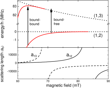
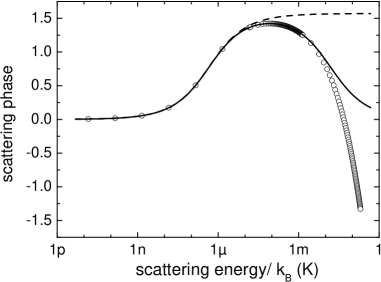
To calculate the scattering phase shifts, we construct a reduced single-channel Hamiltonian to describe the $(1,3)$ continuum. The phase shifts from this model are nearly indistinguishable from those from the full multichannel calculations in this range of $B$-fields. The van der Waals interaction is set to $C_{6}=1393.39(16)$a.u. lic6 , yielding an interaction range of $r_{0}=29.884(3)a_{0}$. The scattering lengths are set to match the values from the multi-channel calculation. The resulting scattering phase shifts from the calculation are compared with the effective range expansion given in Eq. (8) (see Fig. 2). Here, the scattering parameters are based on the $(1,3)$ scattering states at 72.0mT with a scattering length of $a^{\prime}=-7866a_{0}$. The result shows the expected behavior that $k\cot\delta^{\prime}=-1/a^{\prime}$ provides an excellent fit at low scattering energy $E<k_{B}\times 20\mu$ K and the effective range correction works up to $E<k_{B}\times 10$mK. Here $k_{B}$ is Boltzman’s constant.

Figure 2: Comparison of the scattering phase shifts from numerical calculation and from the effective range expansion. The numerical calculation (open circles) is shown together with the predictions from Eq. (8) with (solid line) and without (dashed line) the effective range correction. The scattering parameters are based on ⁶Li in the $(1,3)$ channel near 72.0mT with $a_{13}=-7866a_{0}$.

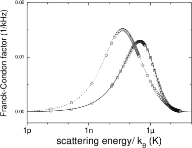
We also compare the Franck-Condon factors obtained from the numerical calculation and from Eq. (10). The numerical calculation is based on an initial bound state in the $(1,2)$ channel and the final state $(1,3)$ continuum, described by the reduced Hamiltonian. We show the calculations at two magnetic fields of 72.0mT and 68.0mT, where the scattering parameters are set according to the multichannel calculations. The results show that Eq. (10) provides an excellent fit to the full bound-free spectra, see Fig. 3.

Figure 3: Comparison of the Franck-Condon factors from numerical calculation and from theory. Numerical calculation at 72.0mT (open squares) and 68.0mT (open circles) are plotted together with the formula Eq. (10) (solid line at 72.0mT and dotted line at 68.0mT). The parameters are $E_{b}=k_{B}\times 16.2\mu$K and $a^{\prime}=25173a_{0}$ at 68.0mT; $E_{b}=k_{b}\times 6.2\mu$K and $a^{\prime}=-7866a_{0}$ at 72.0mT.

IV RF lineshape near a Feshbach resonance

The appearance of the bound-bound transition for only $a^{\prime}>0$ seems to suggest a distinct behavior in rf excitation near the Feshbach resonance where the scattering length changes sign. In this section, we show that the evolution of the rf spectrum is actually continuous when a $B$-field is tuned through the resonance position. We use Eq. (10) andEq. (17) to show the bound-free and bound-bound spectra in the vicinity of a Feshbach resonance.

Figure 4: Transition from a bound-free transition to a bound-bound transition with $E_{b}=1$. For the bound-free transition, the Franck-Condon factor is plotted as a function of $K/E_{b}$. Curves of different $a^{\prime}/a$ are offset and shown in the order of that near a Feshbach resonance in the $A^{\prime}$ channel. (dotted line for the resonance condition) For $a^{\prime}>0$, the locations of the bound-bound transitions are indicated by the sharp peaks. Notably, bound-free transition vanishes at $a^{\prime}=a$.

Figure 4 shows a continuous change near a Feshbach resonance from a bound-free lineshape for $a^{\prime}<0$ to a combination of bound-bound and bound-free transitions for $a^{\prime}>0$. When the scattering length approaches negative infinity, the linewidth of the bound-free lineshape approaches zero as $\sim E_{b^{\prime}}^{2}\sim{a^{\prime}}^{-4}$ and “evolves” into the bound-bound delta function. Remarkably, for $a^{\prime}>0$, the bound-free transition is much weaker. At $a^{\prime}=a$, the bound-free transition is fully suppressed, $\Gamma_{f}=0$.

The vanishing bound-free transition for $a^{\prime}\approx a$ can be understood by the wavefunction overlap given in Eq. (4). As a positive scattering length $a^{\prime}$ indicate a zero in wavefunction near $r\approx a$, the sign change of the scattering wavefunction results in a cancellation in the overlap. Alternatively, we may consider the transition amplitude to the continuum $A^{\prime}$ is exactly cancelled by the Feshbach coupling between molecular state $|m^{\prime}\rangle$ and the continuum $A^{\prime}$. This interference effect results in the Fano-like profile of the peak transition rate near a Feshbach resonance fano (see Fig. 5).

On the other hand, the bound-bound Franck-Condon factor approaches one when $a^{\prime}\approx a$, since both molecular wavefunction are identical for $r>r_{0}$. The peak bound-free transition rates therefore shows a strong asymmetry with respect to the sign of the scattering length, shown in Fig. 5.

Figure 5: Fano profile near a Feshbach resonance in the outgoing channel $A^{\prime}$. The peak Franck-Condon factors with $E_{b}=1$ are calculated for different $a/a^{\prime}$ based on Eq. (10). Near the Feshbach resonance, $a/a^{\prime}$ approaches zero.

Based on the above features, the rf spectroscopy does provides a new strategy to extract various important scattering parameters. In particular, while cold collision measurements are generally insensitive to the sign of the scattering length, our rf excitation spectroscopy is drastically different for the two cases and provides a new tool to probe the scattering properties.

V Comparison with experiment

To compare with the experimental result, we take ⁶Li as a model system and calculate the rf spectra. The experimental spectra are obtained from the Li group in Innsbruck boundbound .

Adopting the convention used in Ref.gap , we define the rf offset energy as $E=E_{RF}-E_{0}=K+E_{b}$. Using Eq. (10), we can rewrite the Franck-Condon factors as

$$F_{f}(E) = \frac{2}{\pi}(1-\frac{a^{\prime}}{a})^{2}\frac{E_{b}^{\prime}E_{b}^{1/2}(E-E_{b})^{1/2}}{E^{2}(E+E_{b}^{\prime}-E_{b})}$$ (19)

$$F_{b}(E) = \frac{4aa^{\prime}}{a+a^{\prime}}\delta(E-E_{b}+E_{b}^{\prime})\mbox{ for }a^{\prime}>0$$ (20)

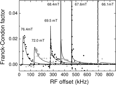
We compare the theoretical curves with the experiment in Fig. 6. An integration bandwidth of 1kHz is assumed. When the magnetic field approaches 69.1mT from high values, the molecular binding energy $E_{b}$ in the $(1,2)$ channel increases (see Fig. 1). This dependence is shown in Fig. 6 as the whole excitation line moves toward higher frequency. At the same time, the lineshape becomes sharper due to the Feshbach resonance in $(1,3)$ channel at 69.1mT. Below 69.1mT, we expect both bound-free and bound-bound transitions are allowed. At 68.4mT, these two components coexist, but cannot be clearly distinguished due to the small binding energy of $E_{b}^{\prime}=h\times 0.5$kHz, lower than the experimental resolution of $\sim 1$kHz. At 67.6mT and 66.1mT, the bound-free transitions are strongly suppressed. The bound-bound transition then shows up as the dominant component in the spectra. The excellent agreement between the experiment and the calculation over a large range of magnetic fields is remarkable. This result strongly suggests that the rf molecular spectroscopy can be used for a precision determination of the atomic interaction parameters boundbound .

Figure 6: RF spectra of ⁶Li₂ molecule at different magnetic field values. Theoretical curves are based on Eq. (19) and Eq. (20) with the binding energies and scattering lengths obtained from the multichannel calculation. To shown both the bound-free and bound-bound spectra, an integration bandwidth of 1kHz is assumed. RF-induced loss on the molecular population at 76.4mT (solid squares), 72.0mT (open squares), 69.5mT (solid circles), 68.4mT (open circles), 67.6mT (solid diamonds) and 66.1mT (open diamonds) are re-scaled. Experiment data are from the Grimm’s group in Innsbruck.

VI Conclusion

We model and evaluate the radio-frequency excitation rates on weakly-bound ultracold molecules in the threshold regime. We derive a simple and analytic form of the bound-free and bound-bound spectral profiles which provide an excellent fit to both the numerical calculation and the recent rf measurements on Li₂ molecules.

An interesting case is studied when a Feshbach resonance occurs in the outgoing channel. We show that the bound-free spectra in the absence of a bound state smoothly evolves into a combination of bound-bound and bound-free spectra when the bound state formed near a Feshbach resonance. The bound-free transition rate strongly depends on the sign of the scattering length and shows a Fano-like structure near the resonance.

We like to point out that the rf spectroscopy based on weakly-bound molecules can be an excellent tool to determine the long-range interaction properties with high precision. From the excitation spectra, the molecular binding energies, the atomic scattering lengths and their signs, and the scattering phase shifts can be determined. Furthermore, in contrast to conventional cold collision measurements, rf transitions on molecules are insensitive to the sample density and temperature, can probe different scattering channels by tuning the rf frequency to different states, and can be implemented instantly without thermalization. Finally, rf transitions between molecular states may also provide a new avenue to transfer the molecular population to low-lying molecular states.

References

- (1) C. Regal, D. Jin, Phys. Rev. Lett. 90, 230404 (2003); C. A. Regal, C. Ticknor, J. L. Bohn, D. S. Jin, Nature 424.
- (2) C. Chin, M. Bartenstein, A. Altmeyer, S. Riedl, S. Jochim, , J. Hecker Denschlag, and R. Grimm, cond-mat/0405632, published online Jul. 22, 2004 (Science Express).
- (3) M. Bartenstein, A. Altmeyer, S. Riedl, R. Geursen, S. Jochim, C. Chin, J. Hecker Denschlag, R. Grimm, A. Simoni, E. Tiesinga, C. J. Williams, and P. S. Julienne, in preparation.
- (4) G.F. Gribakin and V.V. Flambaum, Phys. Rev. A 48, 546 (1993).
- (5) N. F. Mott and H.S.W. Massey, The Theory of Atomic Collisions, (Clarendon Press, Oxford) 1965.
- (6) B. Gao, Phys. Rev. A, 62, 050702(R) (2000).
- (7) P.S. Julienne and F.H. Mies , Phys. Rev. A 30, 831 (1984).
- (8) U. Fano, Phys. Rev. 124, 1866 (1961)
- (9) Z.C. Yan, J.F. Babb, A. Dalgarno, and G.W.F. Drake, Phys. Rev. A 54, 2824 (1996).