Neutron Scattering and Magnetic Observables for S = 1/2 Spin Clusters and Molecular Magnets

Abstract

In this paper we report results for magnetic observables of finite spin clusters composed of S = 1/2 ions. We consider clusters of two, three and four spins in distinct spatial arrangements, with isotropic Heisenberg interactions of various strengths between ion pairs. In addition to the complete set of energy eigenvalues and eigenvectors, specific heat and magnetic susceptibility, we also quote results for the single crystal and powder average inelastic neutron scattering structure factors. Examples of the application of these results to experimental systems are also discussed.

I Introduction

Recent years have seen a rapid increase in the interest in finite quantum spin systems, also known as molecular magnets or nanomagnets Dag96 ; Bar99 ; DiV99 ; Nie00 ; Fur00 ; Bou01 ; Cor02 ; Men99 ; Men00 ; Cif01 . Molecular magnets typically consist of clusters of interacting spins that are magnetically isolated from the other clusters in the molecular solid by nonmagnetic ligands. Formally, molecular magnets are materials in which the ground state has nonzero total spin. Here we generalize this definition to include all systems of largely isolated clusters of interacting quantum spins. These materials are interesting both as simple model systems for the study of quantum magnetism and because they have possible applications as nanoscale computer memory elements DiV99 ; Nie00 . Many realizations of finite spin clusters with various ionic spins, ground state spins and geometries have been reported in the literature; some recent examples with S=1/2 ions are given in Table LABEL:materials.

Theoretical results for the properties of finite S=1/2 quantum spin systems have appeared in several recent references, primarily in the context of experimental studies of specific materials. Dimer results are reported in several studies of the S=1/2 spin dimer VO(HPO₄)$\cdot$0.5H₂O; see for example Johnson et al. Joh84 , Tennant et al. Ten97 and Koo et al. Koo04 . Theoretical properties of S=1/2 spin trimers have similarly been given in studies of candidate trimer materials; see for example Refs.Lub02 ; Qiu02 ; Cag03a ; Cag03b ; Kor04 .

Rather few general theoretical results have been reported for S=1/2 spin tetramers, since the results are more complicated and there are many more independent geometries and sets of superexchanges. Specific cases of tetramers are considered by Procissi et al. Pro04 (S=1/2 square tetramer), Gros et al. Gro03 and Jensen et al. Jen03 (an unsymmetric S=1/2 tetrahedral model of Cu₂Te₂O₅(Br_1-xCl_x)), Kortz et al. Kor04 (unsymmetric tetramer model of K₇Na[Cu₄K₂(H₂O)₆($\alpha$-AsW₉O₃₃)₂]$\cdot$5.5H₂O), and Ciftja Cif01 (symmetric trimer with apical spin). More general reviews of quantum spin systems have been published by Kahn Kah93 (thermodynamics) and Whangbo et al. Wha03 (local origins of magnetism, thermodynamics properties, and materials). Studies of the dynamics of Heisenberg spin clusters using a quasiclassical formalism have been reported in a series of papers by Ameduri, Efremov and Klemm Ame02 ; Efr02 ; Kle02 . Waldmann Wal03 has carried out calcuations of the inelastic neutron structure factor for cyclic Heisenberg spin clusters which are quite similar to the results presented here.

This increased level of interest in molecular magnets motivates more detailed theoretical investigation of the properties of finite quantum spin systems. For simple theoretical models such as the Heisenberg model, clusters that consist of only a few interacting magnetic ions can be treated analytically, and closed-form results can be obtained for many physical observables. One especially interesting quantity is the inelastic neutron scattering structure factor, which is required for the interpretation of inelastic neutron scattering experiments. Inelastic neutron scattering is very well suited to the investigation of magnetic interactions at interatomic scales, since the measured structure factor is sensitive to the local geometry and interactions of the magnetic ions. As this work is intended in part to facilitate future neutron scattering studies, the evaluation of this structure factor is one of our principal concerns.

Table 1: Some examples of small S = 1/2 quantum spin systems.

Material	Spin System	Ground State Stot	Refs.
VO(HPO4)$\cdot$0.5H2O	dimer	0	Joh84 ; Ten97 ; Koo04
Cu3(O2C16H23)${}_{6}\cdot 1.2$C6H12	symmetric trimer	1/2	Cag03a ; Cag03b
Na9[Cu3Na3(H2O)9($\alpha$-AsW9O33)2]$\cdot$26H2O	symmetric trimer	1/2	Kor04
$[$Cu3(cpse)3(H2O)${}_{3}]\cdot 8.5$H2O	symmetric trimer	1/2	Lop02
(CN3H6)4Na2[H4V6O8(PO4)4((OCH2)3CCH2OH)2]$\cdot 14$H2O	isosceles trimer	1/2	Lub02
Na6[H4V6O8(PO4)4((OCH2)3CCH2OH)2]$\cdot 18$H2O	general trimer	1/2	Lub02
K6[V15As6O42(H2O)]$\cdot$8H2O	symmetric trimer + capping hexamers	1/2	Mue88 ; Bar92 ; Gat91 ; Cha02 ; Cha04
NaCuAsO4	linear tetramer	0	Ulu03 ; Nag03
(NHEt3)[V12As8O40(H2O)]$\cdot$H2O.	rectangular tetramer + capping tetramers	0	Bas02
K7Na[Cu4K2(H2O)6($\alpha$-AsW9O33)2]$\cdot$5.5H2O	distorted tetramer	1	Kor04

In this paper we specialize to magnets that are clusters of S=1/2 ions with isotropic Heisenberg interactions, and give analytic results for the properties of dimer, trimer and tetramer clusters with various geometries. After the introduction, in Sec.II we define the Heisenberg model and the observables we evaluate in this work. These include the standard thermodynamic quantities for magnetic materials (partition function, specific heat and magnetic susceptibility), as well as the inelastic neutron scattering structure factors. In Section III we evaluate these quantities for specific spin clusters, which are the spin dimer, symmetric, isosceles and general spin trimers, and three cases of spin tetramers (tetrahedral, rectangular, and alternating linear). We also tabulate all the energy eigenvalues and eigenvectors for each spin system. Section III ends with an application, which is a numerical study of powder inelastic neutron scattering amplitudes in NaCuAsO₄ Ulu03 ; the results appear to support the identification of this material with the alternating linear tetramer model and agree well with the data of Nagler et al. Nag03 . Finally, Section IV discusses several materials which may be candidates for future experimental studies, as well as some interesting directions for future theoretical research.

For reference purposes our principal results for the spin systems considered here are given in a series of tables at the end of the paper. These results are the spectrum of energy eigenvalues and eigenvectors (Table LABEL:wavefunctions1), allowed inelastic neutron scattering transitions between these states (Table LABEL:INSE), and the specific heats (Table LABEL:C_table) and susceptibilities (Table LABEL:chi_table).

Most previous theoretical studies of molecular magnets in the literature have specialized to individual materials and their associated model Hamiltonians. Our results are intended to be sufficiently general so that they should be useful for the interpretation of data on many candidate molecular magnets.

II The Model and Observables

II.1 The Heisenberg Magnet

The nearest-neighbor Heisenberg magnet, which we shall assume as our standard model for molecular magnets, is defined by the Hamiltonian

$${\cal H}=\sum_{<ij>}{\rm J}_{ij}\;\vec{\rm S}_{i}\cdot\vec{\rm S}_{j}$$ (1)

where the superexchange constants $\{{\rm J}_{ij}\}$ are positive for antiferromagnetic interactions and negative for ferromagnetic ones, and $\vec{\rm S}_{i}$ is the quantum spin operator for a spin-1/2 ion at site $i$.

Since this is a rotationally invariant Hamiltonian in spin space, the total spin S_tot is a good quantum number. For the specific cases of dimer, trimer and tetramer clusters of S=1/2 ions that we consider here, the energy eigenstates have the total spin decompositions given below.

$$1/2\otimes 1/2=1\oplus 0,$$ (2)

$$1/2\otimes 1/2\otimes 1/2=3/2\oplus 1/2^{2},$$ (3)

$$1/2\otimes 1/2\otimes 1/2\otimes 1/2=2\oplus 1^{3}\oplus 0^{2}.$$ (4)

Each S_tot multiplet contains 2S${}_{tot}+1$ magnetic states, which are degenerate given an isotropic magnetic Hamiltonian such as the Heisenberg form of Eq.(1).

II.2 Expressions for Observables

The energy eigenstates and eigenvalues may be found by diagonalizing the magnetic Hamiltonian on a convenient basis. (In practice we will employ the usual set of $\hat{z}$-polarized magnetic basis states.) Several physically interesting quantities may be computed directly from the energy eigenvalues; in this work these are the partition function, specific heat and magnetic susceptibility, which are given by

$$Z=\sum_{i=1}^{N}\,e^{-\beta\rm E_{i}}=\sum_{\rm E_{i}}\,(2{\rm S}_{tot}+1)\,e^{-\beta\rm E_{i}}\ ,$$ (5)

$$C=k_{B}\beta^{\,2}\,\frac{d^{2}\!\ln(Z)}{d\beta^{2}}\ ,$$ (6)

and

$$\chi=\frac{\beta}{Z}\sum_{i=1}^{N}\,(M_{z}^{2})_{i}\,e^{-\beta\rm E_{i}}$$

$$=\frac{1}{3}(g\mu_{B})^{2}\frac{\beta}{Z}\sum_{\rm E_{i}}\,(2{\rm S}_{tot}+1)\,({\rm S}_{tot}+1)\,{\rm S}_{tot}\,e^{-\beta\rm E_{i}}\ .$$ (7)

In these central formulas the sum $i=1\dots N$ is over all $N$ independent energy eigenstates (including magnetic substates), the sum $\sum_{\rm E_{i}}$ is over energy levels only, $M_{z}=mg\mu_{B}$ where $m=\rm S_{tot}^{z}/\hbar$ is the integral or half-integral magnetic quantum number, and $g$ is the electron $g$-factor.

In addition to these bulk quantities, we also give results for inelastic neutron scattering intensities. In “spin-only” magnetic neutron scattering at zero temperature, the differential cross section for the inelastic scattering of an incident neutron from a magnetic system in an initial state $|\Psi_{i}\rangle$, with momentum transfer $\hbar\vec{q}$ and energy transfer $\hbar\omega$, is proportional to the neutron scattering structure factor tensor

$$S_{ba}(\vec{q},\omega)=\hskip 85.35826pt$$

$$\int_{-\infty}^{\infty}\!\frac{dt}{2\pi}\ \sum_{\vec{x}{{}_{i}},\vec{x}{{}_{j}}}e^{i\vec{q}\cdot(\vec{x}_{i}-\vec{x}_{j})+i\omega t}\langle\Psi_{i}|\rm S_{b}^{\dagger}(\vec{x}_{j},t)\rm S_{a}(\vec{x}_{i},0)|\Psi_{i}\rangle\ .$$ (8)

The site sums in Eq.(8) run over all magnetic ions in one unit cell, and $a,b$ are the spatial indices of the spin operators.

For transitions between discrete energy levels, the time integral gives a trivial delta function $\delta(\rm E_{f}-\rm E_{i}-\hbar\omega)$ in the energy transfer, so it is useful to specialize to an “exclusive structure factor” for the excitation of states within a specific magnetic multiplet (generically $|\Psi_{f}(\lambda_{f})\rangle$) from the given initial state $|\Psi_{i}\rangle$,

$$S_{ba}^{(fi)}(\vec{q}\,)=\sum_{\lambda_{f}}\ \langle\Psi_{i}|V_{b}^{\dagger}|\Psi_{f}(\lambda_{f})\rangle\ \langle\Psi_{f}(\lambda_{f})|V_{a}|\Psi_{i}\rangle\ ,$$ (9)

where the vector $V_{a}(\vec{q}\,)$ is a sum of spin operators over all magnetic ions in a unit cell,

$$V_{a}=\sum_{{\vec{x}}_{i}}{\rm S}_{a}(\vec{x}_{i})\;e^{i\vec{q}\cdot\vec{x}_{i}}\ .$$ (10)

This exclusive structure factor is related to the exclusive differential inelastic neutron scattering cross section by

$$\frac{\ d\sigma^{(fi)}}{d\Omega}=(\gamma r_{0})^{2}\frac{k^{\prime}}{k}(\delta_{ab}-\hat{q}_{a}\hat{q}_{b})S^{(fi)}_{ba}(\vec{q}\,)|{\rm F}(\vec{q}\,)|^{2}$$ (11)

where $\gamma\approx-1.913$ is the neutron gyromagnetic ratio, $r_{o}=\hbar\alpha/m_{e}c$ is the classical electron radius, $k$ and $k^{\prime}$ are the magnitudes of the initial and final neutron wavevectors, and ${\rm F}(\vec{q}\,)$ is the ionic form factor. (This relation is abstracted from Eq.(7.61) of Ref.Squ78 , specialized to an exclusive process.)

For a rotationally invariant magnetic interaction and an S${}_{tot}=0$ initial state (as is often encountered in T=0 inelastic scattering from an antiferromagnet), only S${}_{tot}~{}=~{}1$ final states are excited, and $S_{ba}^{(fi)}(\vec{q}\,)\propto\delta_{ab}$. In this case we may define a scalar neutron scattering structure factor $S(\vec{q}\,)$ by

$$S_{ba}^{(fi)}(\vec{q}\,)=\delta_{ab}\,S(\vec{q}\,)\ .$$ (12)

The result for $S_{ba}^{(fi)}(\vec{q}\,)$ is more complicated for neutron scattering from a magnetic (S${}_{tot}>0$) initial state. If we assume an isotropic magnetic Hamiltonian and a spherical basis for the spin operators S_a, the tensor $S_{ba}^{(fi)}(\vec{q}\,)$ is diagonal but is not $\propto\delta_{ab}$; it instead has entries that are proportional to a universal function of $\vec{q}$ times a product of Clebsch-Gordon coefficients, since

$$\langle\Psi_{f}(\lambda_{f})|\,V_{a}\,|\Psi_{i}(\lambda_{i})\rangle=\langle{\rm S}_{f}\lambda_{f}|1a\ {\rm S}_{i}\lambda_{i}\rangle\ {\cal V}^{(fi)}(\vec{q}\,)\ ,$$ (13)

where ${\cal V}^{(fi)}(\vec{q}\,)$ is the reduced matrix element for the transition $|\Psi_{i}\rangle\to|\Psi_{f}\rangle$. Here we simplify the presentation by quoting the unpolarized result $\langle S_{ba}^{(fi)}(\vec{q}\,)\rangle$, obtained by summing over final and averaging over initial polarizations. This unpolarized $\langle S_{ba}^{(fi)}(\vec{q}\,)\rangle$ is $\propto\delta_{ab}$, so it suffices to give the function $S(\vec{q}\,)$;

$$\langle S_{ba}^{(fi)}(\vec{q}\,)\rangle=\delta_{ab}\,S(\vec{q}\,)=$$

$$\frac{1}{2\rm S_{i}+1}\sum_{\lambda_{i},\lambda_{f}}\ \langle\Psi_{i}(\lambda_{i})|V_{b}^{\dagger}|\Psi_{f}(\lambda_{f})\rangle\ \langle\Psi_{f}(\lambda_{f})|V_{a}|\Psi_{i}(\lambda_{i})\rangle\ .$$ (14)

If desired, the general results for polarized scattering can be recovered by reintroducing the appropriate Clebsch-Gordon coefficients of Eq.(13) in Eq.(9).

The results given above apply to neutron scattering from single crystals. To interpret neutron experiments on powder samples, we require an orientation average of the unpolarized single-crystal neutron scattering structure factor. We define this powder average by

$${\bar{S}}(q)=\int\frac{d\Omega_{\hat{q}}}{4\pi}\,S(\vec{q}\,)\ .$$ (15)

III Results for Specific Cases

III.1 Spin Dimer

Figure 1: The geometry and energy levels of a Heisenberg spin dimer.

The “minimal” spin cluster model is the S = 1/2 spin dimer (Fig.1), which consists of a single pair of S = 1/2 spins interacting through the Heisenberg Hamiltonian,

$${\cal H}={\rm J}\,\vec{\rm S}_{1}\cdot\vec{\rm S}_{2}\ .$$ (16)

Since this is an isotropic magnetic Hamiltonian, the total spin is a good quantum number, and from the Clebsch-Gordon series $1/2\otimes 1/2=1\oplus 0$ we expect the spectrum to consist of an S${}_{tot}=1$ triplet and an S${}_{tot}=0$ singlet. In a $\hat{z}$-diagonal basis

$$\left[\begin{array}[]{l}|\!\uparrow\uparrow\,\rangle\\ |\!\uparrow\downarrow\,\rangle\\ |\!\downarrow\uparrow\,\rangle\\ |\!\downarrow\downarrow\,\rangle\\ \end{array}\right]$$ (17)

the Hamiltonian matrix is

$${\cal H}={\rm J}\left[\begin{array}[]{cccc}1/4&&&\\ &-1/4&\phantom{-}1/2&\\ &\phantom{-}1/2&-1/4&\\ &&&1/4\end{array}\right].$$ (18)

Diagonalizing this Hamiltonian matrix gives the energy eigenvalues and eigenvectors,

$$\begin{array}[]{l}{\rm E}_{1}=\phantom{-}\frac{1}{4}\,{\rm J}\\ \\ {\rm E}_{0}=-\frac{3}{4}\,{\rm J}\ ,\end{array}$$ (19)

$$\left[\begin{array}[]{l}|\Psi_{1}(+1)\rangle=|\!\uparrow\uparrow\,\rangle\\ \\ |\Psi_{1}(\phantom{+}0)\rangle=\frac{1}{\sqrt{2}}(|\!\uparrow\downarrow\,\rangle+|\!\downarrow\uparrow\,\rangle)\\ \\ |\Psi_{1}(-1)\rangle=|\!\downarrow\downarrow\,\rangle\\ \end{array}\right]$$ (20)

$$|\Psi_{0}\rangle=\frac{1}{\sqrt{2}}(|\!\uparrow\downarrow\,\rangle-|\!\downarrow\uparrow\,\rangle)\ .\quad$$ (21)

The specific heat and magnetic susceptibility for the dimer are especially simple, since there is only a single excited level. The results are (in a dimensionless form)

$$Z=e^{\frac{3}{4}\beta{\rm J}}+3e^{-\frac{1}{4}\beta{\rm J}}$$ (22)

$$\frac{C}{k_{B}}=\;3(\beta{\rm J})^{2}\frac{e^{-\beta{\rm J}}}{\big{(}1+3e^{-\beta{\rm J}}\big{)}^{2}}\ ,$$ (23)

and

$$\frac{\chi}{(g\mu_{B})^{2}/{\rm J}}=\,\;2\beta{\rm J}\,\frac{e^{-\beta{\rm J}}}{(1+3e^{-\beta{\rm J}})}\ .$$ (24)

These results are summarized in Tables LABEL:C_table and LABEL:chi_table, as are the corresponding results we find for the other spin systems considered in this paper. Plots of the dimensionless specific heat and susceptibility of the spin dimer are shown in Figs.2,3.

Figure 2: The magnetic contribution to the specific heat of a spin dimer, Eq.(23) (dimensionless units).

Figure 3: The magnetic susceptibility of a spin dimer, Eq.(24) (dimensionless units).

One may confirm that this specific heat formula gives the correct entropy for a dimer of S=1/2 ions,

$$S=\int_{0}^{\infty}\!\!C\;\frac{d\beta}{\beta}=k_{B}\,2\ln(2)\ .$$ (25)

The corresponding result for a general spin system is

$$S=k_{B}\,\ln({\cal N}/{\cal N}_{0})\ ,$$ (26)

where ${\cal N}$ is the dimensionality of the full Hilbert space and ${\cal N}_{0}$ is the degeneracy of the ground state; for the S=1/2 dimer, ${\cal N}=2^{2}$ and ${\cal N}_{0}=1$.

As an example of the application of the dimer susceptibility of Eq.(24) (known as the Bleaney-Bowers formula Ble52 ), in Fig.4 we show a fit to the susceptibility of the spin dimer VO(HPO₄)$\cdot$0.5H₂O chi_vohpo . (The molar susceptibility shown is related to the single dimer susceptibility of Eq.(24) by $\chi_{molar}=N_{A}/2\cdot\chi$.) The parameters of the fit are $g=2.05$ and J $=7.76$ meV (consistent with the results of inelastic neutron scattering Ten97 ). A 1/T defect contribution was also included in the fit.

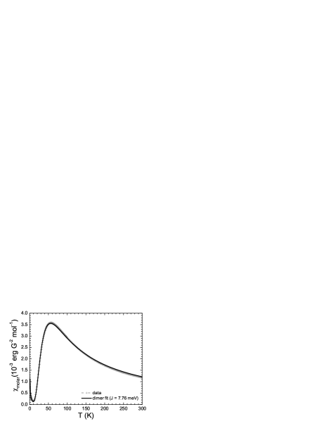
Figure 4: A fit of the dimer susceptibility formula of Eq.(24) to the measured susceptibility of VO(HPO₄)$\cdot$0.5H₂O. A defect term was also included.

Figure 5: The powder average, unpolarized neutron structure factor $\bar{S}(q)$ for a spin dimer with pointlike magnetic ions.

Finally we evaluate the inelastic neutron scattering intensities, which are given by the structure factors of Eqs.(14,15). (A complete set of inelastic neutron scattering transitions for all the spin systems we consider in this work is given in Table LABEL:INSE; typically we will only evaluate the structure factors for the ground state of the antiferromagnetic system.) We evaluate Eq.(14) for the dimer using the energy eigenvectors $|\Psi_{1}(m)\rangle$ and $|\Psi_{0}\rangle$ of Eqs.(20,21). This gives

$$S(\vec{q}\,)=\frac{1}{2}\big{(}1-\cos(\vec{q}\cdot\vec{a}\,)\big{)}$$ (27)

where $\vec{a}=\vec{x}_{1}-\vec{x}_{2}=\vec{x}_{12}$ is a spatial vector that coincides with the dimer. Evidently there should be no excitation of the dimer spin-triplet state when the neutron momentum transfer $\vec{q}$ is perpendicular to the dimer axis $\hat{a}$.

In scattering from powder samples one measures the powder average ${\bar{S}}(q)$ of the structure factor, defined by Eq.(15). For the dimer this is

$${\bar{S}}(q)=\int\frac{d\Omega_{\hat{q}}}{4\pi}\,\frac{1}{2}\,\big{(}1-\cos(\vec{q}\cdot\vec{a}\,)\big{)}=\frac{1}{2}\,\big{(}1-j_{0}(qa)\big{)}$$ (28)

where $j_{0}(x)=\sin(x)/x$ is a spherical Bessel function. This result is shown in Fig.5 for pointlike magnetic ions (F$(\vec{q}\,)=1$). The location of the first maximum, at $q\approx 4.493\,a^{-1}$, provides a convenient estimate of the separation between the interacting ions in the dimer. Of course in real materials the incorporation of ionic form factors will reduce the location of this maximum.

Experimental studies of real magnetic materials typically proceed by establishing the approximate magnetic parameters of a model Hamiltonian through a fit to the susceptibility. Given a model Hamiltonian, one can predict the inelastic neutron scattering structure factor, which is then compared to experiment. (Ideally this is done on single crystal samples, but frequently only powder samples are available.) Unlike the bulk susceptibility, the inelastic neutron scattering structure factor allows a sensitive and microscopic test of the assumed magnetic Hamiltonian, since it is determined by the relative positions of the interacting magnetic ions. The spin-dimer material VO(DPO₄)$\cdot$0.5D₂O provides a recent illustration of the use of inelastic neutron scattering in identifying magnetic interaction pathways; the susceptibility data of Johnson et al. Joh84 was well known to give an excellent fit to the dimer formula Eq.(24), however the separation of the interacting V-V pair inferred from inelastic neutron scattering data Ten97 using Eq.(28) showed that the interacting V-V pair had been misidentified in the literature.

III.2 Trimers

We will consider the most general case of a spin trimer with Heisenberg magnetic interactions. It is useful to present the results as special cases with decreasing symmetry, since the formulas are simpler in the more symmetric cases, and examples of both symmetric and isosceles trimers are known in the literature.

Figure 6: Geometries and energy levels of (a) symmetric, (b) isosceles and (c) general trimer systems. These systems have one S${}_{tot}=\frac{3}{2}$ multiplet and two S${}_{tot}=\frac{1}{2}$ multiplets.

III.2.1 Symmetric Trimer

The completely symmetric, equilateral trimer has equal magnetic couplings and bond lengths between all three pairs of spins. The Hamiltonian for this model is

$${\cal H}={\rm J}\,\Big{(}\vec{\rm S}_{1}\cdot\vec{\rm S}_{2}+\vec{\rm S}_{2}\cdot\vec{\rm S}_{3}+\vec{\rm S}_{3}\cdot\vec{\rm S}_{1}\Big{)}\ .$$ (29)

Since this Hamiltonian is invariant under any permutation of the three spin labels, it has a discrete S₃ symmetry in addition to the magnetic rotational symmetry. In an S_z-diagonal basis

$$\left[\begin{array}[]{l}|\!\uparrow\uparrow\uparrow\,\rangle\\ |\!\uparrow\uparrow\downarrow\,\rangle\\ |\!\uparrow\downarrow\uparrow\,\rangle\\ |\!\downarrow\uparrow\uparrow\,\rangle\\ |\!\uparrow\downarrow\downarrow\,\rangle\\ |\!\downarrow\uparrow\downarrow\,\rangle\\ |\!\downarrow\downarrow\uparrow\,\rangle\\ |\!\downarrow\downarrow\downarrow\,\rangle\\ \end{array}\right]$$ (30)

the Hamiltonian matrix is

$${\rm J}\left[\begin{array}[]{cccccccc}3/4&&&&&&&\\ &-1/4&\phantom{-}1/2&\phantom{-}1/2&&&&\\ &\phantom{-}1/2&-1/4&\phantom{-}1/2&&&&\\ &\phantom{-}1/2&\phantom{-}1/2&-1/4&&&&\\ &&&&-1/4&\phantom{-}1/2&\phantom{-}1/2&\\ &&&&\phantom{-}1/2&-1/4&\phantom{-}1/2&\\ &&&&\phantom{-}1/2&\phantom{-}1/2&-1/4&\\ &&&&&&&3/4\\ \end{array}\right]_{\ .}$$ (39)

(40)

This matrix is block diagonal within subspaces of definite S${}_{z\,tot}$, as expected for a rotationally invariant Hamiltonian. The energy levels of the symmetric trimer are shown in Fig.6a. For the J $>0$ (antiferromagnetic) case the ground state is a quadruplet (the two S${}_{tot}=1/2$ multiplets are degenerate), and there is an energy gap of $\frac{3}{2}$J to the S${}_{tot}=3/2$ excited state. Representative symmetric trimer energy eigenstates (those with maximum S${}_{z\,tot}$) are given in Table LABEL:wavefunctions1. Since the two S${}_{tot}=1/2$ levels are degenerate, there is no unique ground state for this system; we use the Jacobi $|\rho\rangle=|(12)_{A}\rangle$ and $|\lambda\rangle=|(12)_{S}\rangle$ three-body basis states of definite $(12)$-exchange symmetry as our two independent basis vectors.

We may determine the specific heat and magnetic susceptibility of the symmetric trimer from these energy levels, using Eqs.(6,7). The results are

$$\frac{C}{k_{B}}=\frac{9}{4}(\beta\rm J)^{2}\frac{e^{-\frac{3}{2}\beta\rm J}}{(1+e^{-\frac{3}{2}\beta\rm J})^{2}}$$ (41)

and

$$\frac{\chi}{(g\mu_{B})^{2}/{\rm J}}=\frac{1}{4}\,\beta\rm J\,\frac{(1+5e^{-\frac{3}{2}\beta\rm J})}{(1+e^{-\frac{3}{2}\beta\rm J})}\ .$$ (42)

It is notable that the integral of this specific heat gives an entropy of

$$S=\int_{0}^{\infty}\!\!C\;\frac{d\beta}{\beta}=k_{B}\ln(2)$$ (43)

which is only half as large as the entropy of the dimer, despite the larger trimer Hilbert space, ${\cal N}=2^{3}=8$. The lower entropy is due to the fourfold degenerate ground state of this highly frustrated system;

$$S=k_{B}\ln({\cal N}/{\cal N}_{0})=k_{B}\ln(2^{3}/4)=k_{B}\ln(2)\ .$$ (44)

The susceptibility of the symmetric trimer, Eq.42, agrees with Eq.2 of Veit et al. Vei86 (after specializing to a single $g$-factor and a change of variables). This result is shown in Fig.7. Note that $\chi(T)$ diverges as we approach zero temperature, since the ground state has nonzero spin. This divergence is present independent of whether the intrinsic spin-spin coupling J is antiferromagnetic (as we normally assume) or ferromagnetic, since both cases have ground states of nonzero spin. A more detailed comparison of the susceptibility suffices to distinguish these; see the inset of Fig.7, which shows $\chi$T versus T for both cases. At high temperatures the spin-spin coupling J is unimportant, and both results approach the same Curie’s law limit.

Figure 7: The magnetic susceptibility of a symmetric trimer. The inset shows $\chi T$ versus $T$ for ferromagnetic (dashed) and antiferromagnetic (solid) couplings.

Next we consider the neutron scattering structure factors for the symmetric trimer. Since this system has two degenerate S_tot = 1/2 ground states and a single S_tot = 3/2 excitation, there are two distinct exclusive inelastic neutron structure factors but only a single transition energy, ${\rm E}_{1}-{\rm E}_{0}=\frac{3}{2}\,$J. We have chosen $|\rho\rangle$ and $|\lambda\rangle$ basis states for our orthogonal S_tot = 1/2 eigenstates, and will give neutron structure factors for each of these. The same structure factors follow for the isosceles trimer, although in that case the two S_tot = 1/2 states are nondegenerate.

The structure factors for excitation of the S_tot = 3/2 $|\sigma\rangle$ level (using Eq.(14)) are given by

$$S^{(\rho\to\sigma)}(\vec{q}\,)=\frac{1}{3}\big{(}1-\cos(\vec{q}\cdot\vec{x}_{12})\big{)}\ ,$$ (45)

$$S^{(\lambda\to\sigma)}(\vec{q}\,)=\hskip 85.35826pt$$

$$\frac{1}{3}\,\big{(}1+\frac{1}{3}\cos(\vec{q}\cdot\vec{x}_{12})-\frac{2}{3}\cos(\vec{q}\cdot\vec{x}_{13})-\frac{2}{3}\cos(\vec{q}\cdot\vec{x}_{23})\big{)}\ .$$ (46)

These results may be understood in terms of the different natures of the $|\rho\rangle$ and $|\lambda\rangle$ initial states. In the $|\rho\rangle$ ground state the (12)-dimer is in a pure S${}_{(12)}=0$ state, which must be excited to S${}_{(12)}=1$ to couple to the $|\sigma\rangle$ excited state. The $|\rho\rangle\to|\sigma\rangle$ excitation problem is thus identical to the dimer problem, to within an overall constant. It follows that $S^{(\rho\to\sigma)}(\vec{q}\,)$ is proportional to the dimer structure factor of Eq.(27). In contrast, in the $|\lambda\rangle$ initial state the (12)-dimer is pure S${}_{(12)}=1$ and the (23)- and (31)-dimers have amplitudes to be in both spin 0 and 1, so there are contributions to $S^{(\lambda\to\sigma)}$ due to the excitation of each of the three dimer subsystems.

As $S^{(\rho\to\sigma)}$ and $S^{(\lambda\to\sigma)}$ differ considerably for moderate $qa$ it will certainly be possible to distinguish between $|\rho\rangle$ and $|\lambda\rangle$ states from their single crystal structure factors. The powder averages however are identical, and cannot be distinguished experimentally;

$${\bar{S}}^{(\rho\to\sigma)}(q)={\bar{S}}^{(\lambda\to\sigma)}(q)=\frac{1}{3}\big{(}1-j_{0}(qa)\big{)}\ .$$ (47)

These powder structure factors are identical because of the identical dimer lengths, $r_{12}=r_{23}=r_{31}=a$, so the powder average of each cosine in Eqs.(45,46) gives the same $j_{0}(qa)$ Bessel function. The dependence $(1-j_{0}(qa))$ follows from the requirement that $\bar{S}(0)=0$.

As we shall discuss in the next section, an isosceles trimer would be a more favorable system for the identification of $|\rho\rangle$ and $|\lambda\rangle$ initial states in inelastic neutron scattering; these levels are nondegenerate in the isosceles system, and the $|\rho\rangle\to|\sigma\rangle$ and $|\lambda\rangle\to|\sigma\rangle$ powder average structure factors are no longer equal, due to the different leg lengths.

III.2.2 Isosceles Trimer

The isosceles spin trimer, Fig. 6b, has two equal magnetic interactions and bond lengths. The Hamiltonian is given by

$${\cal H}={\rm J}\Big{(}\vec{\rm S}_{1}\cdot\vec{\rm S}_{2}+\alpha\big{(}\vec{\rm S}_{2}\cdot\vec{\rm S}_{3}+\vec{\rm S}_{3}\cdot\vec{\rm S}_{1}\big{)}\Big{)}\ .$$ (48)

To find the energy eigenvalues of this Hamiltonian it suffices to consider the S${}_{z\,tot}=+1/2$ sector, since the S${}_{tot}=1/2$ and $3/2$ multiplets both have S${}_{z\,tot}=+1/2$ members. The remaining symmetry of this problem suggests that we use the three $\{|{\rm S}_{tot},+1/2\rangle\}$ energy eigenstates of the symmetric trimer as our basis,

$$\left[\begin{array}[]{l}|\sigma(3/2,+1/2)\rangle=\sqrt{\frac{1}{3}}\ (|\!\uparrow\uparrow\downarrow\,\rangle+|\!\uparrow\downarrow\uparrow\,\rangle+|\!\downarrow\uparrow\uparrow\,\rangle)\\ |\lambda(1/2,+1/2)\rangle=\sqrt{\frac{1}{6}}\ (|\!\uparrow\downarrow\uparrow\,\rangle+|\!\downarrow\uparrow\uparrow\,\rangle-2|\!\uparrow\uparrow\downarrow\,\rangle)\\ |\rho(1/2,+1/2)\rangle=\sqrt{\frac{1}{2}}\ (|\!\uparrow\downarrow\uparrow\,\rangle-|\!\downarrow\uparrow\uparrow\,\rangle)\\ \end{array}\right]_{\ .}$$ (49)

The Hamiltonian is necessarily diagonal on this basis, since these three basis states have different values of the conserved quantities S_tot and $(12)$-exchange symmetry. The result is

$${\cal H}=\frac{1}{4}\,{\rm J}\left[\begin{array}[]{ccc}1+2\,\alpha&&\\ &1-4\,\alpha&\\ &&-3\end{array}\right]_{\ .}$$ (53)

The two S${}_{tot}=\frac{1}{2}$ levels are split as a result of the reduced symmetry of the isosceles trimer; the full S₃ symmetry of the symmetric trimer has been reduced to S₂ ($(12)$-exchange symmetry), and since S₂ is Abelian no degeneracies follow from this symmetry.

The specific heat and susceptibility of the isosceles trimer, which follow from the energy levels of Eq.(53) and the formulas Eqs.(6,7), are given in Tables LABEL:C_table and LABEL:chi_table. The susceptibility agrees with the earlier result of Veit et al. Vei86 . Note that one recovers the symmetric trimer result in the limit $\alpha=1$.

We have confirmed by numerical integration of the rather complicated isosceles trimer specific heat formula given in Table LABEL:C_table that the entropy of the isosceles trimer satisfies

$$\frac{S}{k_{B}}=\int_{0}^{\infty}\!\!\frac{C}{k_{B}}\;\frac{d\beta}{\beta}=\begin{cases}2\ln(2)&\text{$\alpha\neq 1$}\\ \phantom{2}\ln(2)&\text{$\alpha=1$\ ,}\end{cases}$$ (54)

as expected from Eq.(26) for an eight-dimensional Hilbert space which has a fourfold-degenerate ground state for $\alpha=1$, and a twofold-degenerate ground state otherwise.

Although the magnetic contribution to the specific heat is usually masked by much larger phonon contributions, we note in passing that one may separate magnetic contributions experimentally by subtracting the specific heats in zero and nonzero magnetic fields. This approach was used recently by Luban et al. Lub02 to study an S=1/2 V⁴⁺ vanadium trimer, (CN₃H₆)₄Na₂[H₄V₆O₈(PO₄)₄ ((OCH₂)₃CCH₂OH)₂]$\cdot 14$H₂O (their material 1), which appears to be an accurate realization of the isosceles Heisenberg trimer.

As we found for the symmetric trimer, the susceptibility of the isosceles trimer also diverges as T approaches zero, since the system has a magnetized ground state. The rate of divergence with T can again be used to distinguish between ferromagnetic and antiferromagnetic couplings (which have S${}_{tot}=3/2$ and S${}_{tot}=1/2$ ground states respectively), as shown in Fig.7 for the symmetric trimer. This behavior is evident in the susceptibility of material 1 of Luban et al. Lub02 ; in Fig.3 of this reference one can see that $\chi$T for this material clearly follows the lower trimer curve, confirming that it is accurately described by the antiferromagnetic isosceles trimer model (with an S${}_{tot}=1/2$ ground state).

There are three inelastic transitions excited by neutron scattering from an isosceles spin trimer, $|\rho\rangle\to|\sigma\rangle$, $|\lambda\rangle\to|\sigma\rangle$ and $|\rho\rangle\to|\lambda\rangle$. The first two were considered in the discussion of the symmetric trimer, and the results for the isosceles trimer are identical (except that the $\Delta E$ values of the transitions differ). The $|\rho\rangle\to|\lambda\rangle$ transition was not considered previously because these states are degenerate in the symmetric trimer. The result we find for the structure factor of this transition is

$$S^{(\rho\to\lambda)}(\vec{q}\,)=\frac{1}{6}\Big{(}1-\cos(\vec{q}\cdot\vec{x}_{12})\Big{)}\ .$$ (55)

This has the same form as the dimer and $|\rho\rangle\to|\sigma\rangle$ structure factors because it also involves the excitation of the S₍₁₂₎ = 0 (12)-dimer to an S₍₁₂₎ = 1 state. It can evidently be distinguished from the $|\rho\rangle\to|\sigma\rangle$ transition by the overall intensity, but not by the functional dependence on $q$.

To illustrate these single crystal structure factors, in Fig.8 we show the two ground state structure factors for the previously cited V₆ isosceles trimer (material 1 of Luban et al. Lub02 ). The parameters are $a=3.22$ Å  and $b=3.364$ Å. We show the predictions of Eqs.(46,55) for in-plane scattering, with momentum transfer $q=\pi/a$. Since this material has two strong bonds and a weak dimer $(\alpha\approx 9)$ Lub02 , $|\lambda\rangle$ should be the ground state, and the $|\lambda\rangle\to|\rho\rangle$ and $|\lambda\rangle\to|\sigma\rangle$ transitions shown in the figure should both be observable (These are expected at 4.2 meV and 7.0 meV respectively, given the parameters of Luban et al.) The very different angular distributions predicted for the scattered neutrons show that it should be straightforward to distinguish between these transitions in an inelastic neutron scattering experiment, given a single crystal of this or a similar trimer material.

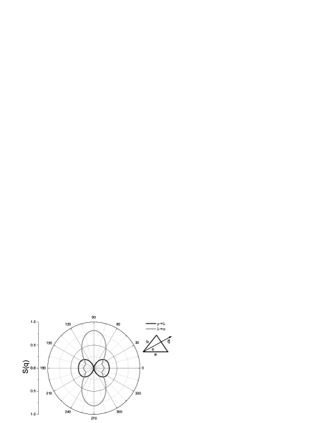
Figure 8: The unpolarized structure factors $\{S(\vec{q})\}$ (proportional to the angular scattering intensities) predicted for inelastic neutron scattering from the $|\lambda\rangle$ ground state of a single crystal of an isosceles trimer material (see text).

The powder average eliminates much of the difference between these neutron scattering transitions, although it still should be possible to distinguish them experimentally. On carrying out the powder average we find

$$\begin{array}[]{ccc}&{\bar{S}}^{(\rho\to\sigma)}(q)=&\frac{1}{3}\big{(}1-j_{0}(qa)\big{)}\phantom{\ .}\\ \\ &{\bar{S}}^{(\lambda\to\sigma)}(q)=&\frac{1}{3}\big{(}1+\frac{1}{3}j_{0}(qa)-\frac{4}{3}j_{0}(qb)\big{)}\\ \\ &{\bar{S}}^{(\rho\to\lambda)}(q)=&\frac{1}{6}\big{(}1-j_{0}(qa)\big{)}\phantom{\ .}\ .\\ \end{array}$$ (61)

In the symmetric limit $b/a=1$ these transitions are proportional to the same function, $1-j_{0}(qa)$; at best it may be possible to distinguish the $|\rho\rangle\to|\lambda\rangle$ transition from the others through their relative intensities. However for significantly different leg lengths the $|\lambda\rangle\to|\sigma\rangle$ powder average structure factor may differ enough from the $1-j_{0}(qa)$ of the $|\rho\rangle\to|\sigma\rangle$ and $|\rho\rangle\to|\lambda\rangle$ transitions to distinguish them. As an example, in Fig.9 we show the powder structure factors of Eq.(61) for the three transitions, for an elongated triangle with $b/a=2$. (These results are independent of the magnetic coupling ratio $\alpha$.) As there is considerable variation in form and magnitude between these powder structure factors, it should be possible to distinguish them experimentally in similar isosceles trimer materials. If more than one transition is clearly observed, it may also be useful to compare structure factor ratios, to eliminate the effect of ionic form factors.

Figure 9: The powder average inelastic neutron structure factor $\bar{S}(q)$ for the three allowed transitions of an isosceles trimer, with $b/a=2$.

III.2.3 General Trimer

The general trimer of Fig.6c has three different magnetic couplings and ion pair separations, and is described by the Hamiltonian

$${\cal H}={\rm J}\Big{(}\vec{\rm S}_{1}\cdot\vec{\rm S}_{2}+\alpha_{23}\,\vec{\rm S}_{2}\cdot\vec{\rm S}_{3}+\alpha_{31}\,\vec{\rm S}_{3}\cdot\vec{\rm S}_{1}\Big{)}\ .$$ (62)

This system is also discussed by Qiu et al. Qiu02 in the context of La₄Cu₃MoO₁₂, which they model as a two dimensional coupled array of S=1/2 trimers.

We may again determine all the trimer energy eigenvalues by specializing to the S${}_{z\,tot}=+1/2$ sector and using the symmetric trimer basis of Eq.(49), which gives the Hamiltonian matrix

$${\cal H}=\frac{1}{4}\,{\rm J}\left[\begin{array}[]{ccc}1+\alpha_{s}&&\\ &1-2\alpha_{s}&\sqrt{3}\,\alpha_{d}\\ &\sqrt{3}\,\alpha_{d}&-3\end{array}\right]$$ (66)

where $\alpha_{s}=\alpha_{31}+\alpha_{23}$ and $\alpha_{d}=\alpha_{31}-\alpha_{23}$. The $|\sigma\rangle$ basis states again must be energy eigenstates, since they are the only S${}_{tot}=3/2$ states in the Hilbert space. They have energies of

$${\rm E}_{\frac{3}{2}}=\frac{1+\alpha_{s}}{4}\,{\rm J}\,\ .$$ (67)

The S${}_{tot}=1/2$ basis states $|\rho\,\rangle$ and $|\lambda\rangle$ mix in this problem, since the general trimer Hamiltonian with $\alpha_{23}\neq\alpha_{31}$ breaks (12)-exchange symmetry. The resulting energies are

$${\rm E}_{\frac{1}{2},\,\{{1\atop 2}\}}=-\frac{(1+\alpha_{s}\pm\sqrt{(2-\alpha_{s})^{2}+3\,\alpha_{d}^{2}\,}\,)}{4}\;{\rm J}\ .$$ (68)

The specific heat and susceptibility of the general trimer follow from the energy levels of Eqs.(67,68) and the formulas Eqs.(6,7). The resulting expressions are given in Tables LABEL:C_table and LABEL:chi_table. One may confirm recovery of the isosceles and symmetric trimer results as special cases of these results. We have also confirmed by numerical integration that the rather lengthly general trimer specific heat formula given in Table LABEL:C_table leads to an entropy of $S=k_{B}\,2\ln(2)$, provided that at least one of the parameters $\alpha_{23}$ and $\alpha_{31}$ differs from unity.

The neutron scattering structure factors for the general trimer involve coherent superpositions of the previously derived $|\rho\rangle$ and $|\lambda\rangle$ excitation functions, since the energy eigenstates are superpositions of these basis states. The S${}_{tot}=1/2$ energy eigenstates of Eq.(66) are explicitly

$$|\Psi_{\frac{1}{2},1}\rangle=-\sin(\theta)|\lambda\rangle+\cos(\theta)|\rho\rangle$$ (69)

and

$$|\Psi_{\frac{1}{2},2}\rangle=+\cos(\theta)|\lambda\rangle+\sin(\theta)|\rho\rangle\ ,$$ (70)

where the mixing angle $\theta$ satisfies

$$\tan(\theta)=\frac{x}{1+\sqrt{1+x^{2}}}$$ (71)

with $x=\sqrt{3}\,\alpha_{d}/(2-\alpha_{s})$. The S${}_{tot}=3/2$ energy eigenstate is, as for all the trimers we have considered,

$$|\Psi_{\frac{3}{2}}\rangle=|\sigma\rangle\ .$$ (72)

The structure factor for the transition from the S${}_{tot}=1/2$ state $|\Psi_{\frac{1}{2},1}\rangle$ to the S${}_{tot}=3/2$ state is given by

$$S^{(\Psi_{\frac{1}{2},1}\to\Psi_{\frac{3}{2}})}(\vec{q}\,)=\frac{1}{3}\bigg{(}\big{(}1-\frac{1}{3}(C_{12}+C_{23}+C_{31})\big{)}$$

$$+\frac{1}{3}\,{\cal C}_{2}\,\big{(}\,C_{31}+C_{23}-2\,C_{12}\big{)}+\frac{1}{\sqrt{3}}\,{\cal S}_{2}\,\big{(}C_{31}-C_{23}\big{)}\bigg{)}$$ (73)

where $C_{ij}=\cos(\vec{q}\cdot\vec{x}_{ij})$, ${\cal C}_{2}=\cos(2\theta)$ and ${\cal S}_{2}=\sin(2\theta)$. The structure factor for the second transition, $\Psi_{\frac{1}{2},2}\to\Psi_{\frac{3}{2}}$, follows from Eq.(73) on changing the overall signs of the ${\cal C}_{2}$ and ${\cal S}_{2}$ terms. The third transition, between the two S${}_{tot}=1/2$ states, has the structure factor

$$S^{(\Psi_{\frac{1}{2},1}\to\Psi_{\frac{1}{2},2})}(\vec{q}\,)=\frac{1}{6}\bigg{(}\big{(}1-\frac{1}{3}(C_{12}+C_{23}+C_{31})\big{)}$$

$$+\frac{1}{3}\,{\cal C}_{4}\,\big{(}C_{31}+C_{23}-2\,C_{12}\big{)}+\frac{1}{\sqrt{3}}\,{\cal S}_{4}\,\big{(}C_{31}-C_{23}\big{)}\bigg{)}\ ,$$ (74)

where the new quantities are ${\cal C}_{4}=\cos(4\theta)$ and ${\cal S}_{4}=\sin(4\theta)$. One may confirm that the previously derived symmetric and isosceles trimer structure factors of Eqs.(45,46,55) follow from these general trimer results in the limit $\theta\to 0$.

The powder averages of these general trimer unpolarized structure factors may also be evaluated; the result for the transition $\Psi_{\frac{1}{2},1}\to\Psi_{\frac{3}{2}}$ is

$${\bar{S}}^{(\Psi_{\frac{1}{2},1}\to\Psi_{\frac{3}{2}})}(\vec{q}\,)=\frac{1}{3}\bigg{(}1-\frac{(1+2\,{\cal C}_{2})}{3}\,j_{0}(qr_{12})$$

$$-\frac{(1-{\cal C}_{2}+\sqrt{3}\,{\cal S}_{2})}{3}\,j_{0}(qr_{23})-\frac{(1-{\cal C}_{2}-\sqrt{3}\,{\cal S}_{2})}{3}\,j_{0}(qr_{31})\bigg{)}\ .$$ (75)

The powder average results for the two remaining transitions can be obtained from Eq.(75) by simple substitutions. To obtain ${\bar{S}}^{(\Psi_{\frac{1}{2},2}\to\Psi_{\frac{3}{2}})}$ simply change the overall signs of ${\cal C}_{2}$ and ${\cal S}_{2}$ in Eq.(75), and to obtain ${\bar{S}}^{(\Psi_{\frac{1}{2},1}\to\Psi_{\frac{1}{2},2})}$, divide Eq.(75) by a factor of two and replace ${\cal C}_{2}$ and ${\cal S}_{2}$ by ${\cal C}_{4}$ and ${\cal S}_{4}$ respectively.

These results will be useful for the interpretation of neutron scattering data on real materials. One example of a candidate general trimer is the V₆ material 2 of Luban et al. Lub02 , Na₆[H₄V₆O₈(PO₄)₄((OCH₂)₃ CCH₂OH)₂]$\cdot 18$H₂O. This compound has three distinct V-V separations between the S=1/2 V⁴⁺ ions within each vanadium trimer, $3.212$ Å, $3.252$ Å and $3.322$ Å.

III.3 Tetramers

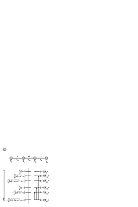
Figure 10: Energy level diagrams for (a) the tetrahedron, (b) the rectangular tetramer, and (c) the linear (dimer-pair) tetramer.

We will consider three S = 1/2 tetramer spin clusters of decreasing symmetry, the regular tetrahedron, the rectangular tetramer, and the linear (dimer-pair) tetramer. Our definitions for the magnetic couplings and geometry of these systems are shown in Fig.10. As with the dimer and trimer systems we will give results for the partition function, specific heat, magnetic susceptibility and neutron inelastic scattering structure factors, the latter for both single crystal and powder average cases.

III.3.1 Tetrahedron

This system has four S = 1/2 ions at the vertices of a regular tetrahedron, with Heisenberg interactions of strength J between each pair of ions (see Fig.10a). The Hamiltonian of this system is given by

$${\cal H}={\rm J}\sum_{i,j=1\atop i<j}^{4}{\vec{\rm}S}_{i}\cdot{\vec{\rm}S}_{j}\ .$$ (76)

The invariance of this Hamiltonian under permutation of any site labels implies an S₄ symmetry, in addition to the spin rotation symmetry SU(2). Since the group S₄ is non-Abelian and has irreducible representations of dimensionality ${\underline{1}}$, ${\underline{2}}$ and ${\underline{3}}$, we anticipate that one may find twofold and threefold degeneracies in the spectrum of tetrahedron energy eigenstates. We will see that this is indeed the case.

As with the dimer and symmetric trimer we may determine the energy eigenvalues of this system by simply squaring the total spin operator $\vec{\rm}S_{tot}=\sum_{i=1}^{n}\vec{\rm}S_{i}$, which gives for this case

$$\rm E_{{\rm S}_{tot}}=\frac{1}{2}\,{\rm J}\Big{(}\,{\rm S}_{tot}({\rm S}_{tot}+1)-3\Big{)}=\begin{cases}+\frac{3}{2}\,\rm J&\text{S${}_{tot}=2$}\\ -\frac{1}{2}\,\rm J&\text{S${}_{tot}=1$}\\ -\frac{3}{2}\,\rm J&\text{S${}_{tot}=0$.}\end{cases}$$ (77)

The Clebsch-Gordon series of Eq.(4) implies that these S${}_{tot}=1$ and S${}_{tot}=0$ energy levels are respectively threefold and twofold degenerate.

Given these energy levels, the specific heat and susceptibility of the tetrahedron may then be determined using Eqs.(6,7), with the results

$$\frac{C}{k_{B}}=\frac{9}{2}(\beta\rm J)^{2}e^{-\beta\rm J}\;\frac{(1+5e^{-2\beta\rm J}+10e^{-3\beta\rm J})}{\left(1+\frac{9}{2}e^{-\beta\rm J}+\frac{5}{2}e^{-3\beta\rm J}\right)^{2}}$$ (78)

and

$$\frac{\chi}{(g\mu_{B})^{2}/\rm J}=3\beta\rm J\,e^{-\beta\rm J}\frac{(1+\frac{5}{3}e^{-2\beta\rm J})}{\left(1+\frac{9}{2}e^{-\beta\rm J}+\frac{5}{2}e^{-3\beta\rm J}\right)}\ .$$ (79)

These quantities are shown in Fig.11 and Fig.12 respectively. The specific heat of the tetrahedron gives an entropy of $S=k_{B}\,3\ln(2)$, as expected for a 16-dimensional Hilbert space and a doubly-degenerate ground state.

Note that the susceptibility is rather similar to that of the spin dimer, since the tetrahedron also has an S${}_{tot}=0$ ground state and a gap of J to the magnetized S${}_{tot}=1$ excited states. (The fact that the ground state is twofold degenerate does not affect this result, since both are S${}_{tot}=0$ states and neither makes a contribution to the susceptibility.)

Figure 11: Magnetic contribution to the specific heat of a regular tetrahedron.

Figure 12: Susceptibility of a regular tetrahedron.

Determination of the energy eigenvectors requires diagonalization of the Hamiltonian on a specific basis. Operating on our $|(12)(34)\rangle$ dimer basis of Eqs.(A.8-A.10) with the tetrahedron Hamiltonian, Eq.(76), we find that the Hamiltonian matrix is already fully diagonal; each of these basis states is an energy eigenvector of the tetrahedron Hamiltonian.

In our discussion of neutron scattering structure factors of the tetrahedron and the other spin tetramers considered in this paper, we will specialize to S${}_{\,tot}=0$ initial states. Structure factors for S${}_{\,tot}>0$ initial states, which are of interest for systems with magnetized ground states and at finite temperatures, and can be derived using similar methods.

The tetrahedron has two degenerate ground states, which we take to be $|\Psi_{0,1}\rangle=|\rho\rho\rangle$ and $|\Psi_{0,2}\rangle=|\sigma\sigma\rangle_{0}$. The three degenerate S${}_{\,tot}=1$ excited states, which can be reached from the S${}_{\,tot}=0$ levels using inelastic neutron scattering, are taken to be $|\Psi_{1,1}\rangle=|(\rho\sigma)_{S}\rangle$, $|\Psi_{1,2}\rangle=|(\rho\sigma)_{A}\rangle$ and $|\Psi_{1,3}\rangle=|(\sigma\sigma)_{S}\rangle_{1}$. The choice of this specific set of initial and final states is rather arbitrary; in a real material we would expect a spontaneous distortion of the lattice, which would select nearly degenerate energy eigenstates that need not be these specific basis states. However these will suffice to illustrate the neutron scattering structure factors expected for nearly tetrahedral systems.

The single crystal structure factors for all of these transitions may be read directly from Eqs.(A.16-A.23). For example, the transition $|\Psi_{0,1}\rangle\to|\Psi_{1,1}\rangle$ is specified by the matrix element of Eq.(A.16); using the structure factor definition in Eq.(14), we find

$$\hskip-113.81102ptS^{(\Psi_{0,1}\to\Psi_{1,1})}(\vec{q}\,)=1/2$$

$$-\big{(}C_{12}-C_{13}+C_{14}+C_{23}-C_{24}+C_{34}\big{)}/4$$ (80)

where as before $C_{ij}=cos(\vec{q}\cdot\vec{x}_{ij})$. This characteristic angular distribution and its five partner distributions could be used in an inelastic neutron scattering experiment from a single crystal sample to characterize the spin states of the individual S${}_{\,tot}=0$ and S${}_{\,tot}=1$ levels. (Note however that one specific transition, $|\Psi_{0,1}\rangle\to|\Psi_{1,3}\rangle$, has a zero matrix element.)

The powder average structure factors for a tetrahedron are much less characteristic. Since there is only a single ion pair separation, each cosine in the single crystal structure factors such as Eq.(80) powder-averages to the same factor of $j_{0}(qa)$. This gives a powder structure factor that is proportional to $1-j_{0}(qa)$ for each transition, just as we found for the dimer and symmetric tetramer; only the overall coefficients distinguish the different transitions. These results are

$$\begin{array}[]{ccc}&{\bar{S}}^{(\Psi_{0,1}\to\Psi_{1,1})}(q)=&\frac{1}{2}\big{(}1-j_{0}(qa)\big{)}\phantom{\ .}\\ \\ &{\bar{S}}^{(\Psi_{0,1}\to\Psi_{1,2})}(q)=&\frac{1}{2}\big{(}1-j_{0}(qa)\big{)}\phantom{\ .}\\ \\ &{\bar{S}}^{(\Psi_{0,1}\to\Psi_{1,3})}(q)=&0\phantom{\ .}\\ \\ &{\bar{S}}^{(\Psi_{0,2}\to\Psi_{1,1})}(q)=&\frac{1}{6}\big{(}1-j_{0}(qa)\big{)}\phantom{\ .}\\ \\ &{\bar{S}}^{(\Psi_{0,2}\to\Psi_{1,2})}(q)=&\frac{1}{6}\big{(}1-j_{0}(qa)\big{)}\phantom{\ .}\\ \\ &{\bar{S}}^{(\Psi_{0,2}\to\Psi_{1,3})}(q)=&\frac{2}{3}\big{(}1-j_{0}(qa)\big{)}\ .\\ \end{array}$$ (92)

A generalization of the tetrahedron problem in which the Hamiltonian has couplings of strength $\alpha$J between ions in different dimers may also be of interest. This generalized Hamiltonian is

$${\cal H}(\alpha)={\rm J}\Big{(}\big{(}\vec{\rm S}_{1}\cdot\vec{\rm S}_{2}+\vec{\rm S}_{3}\cdot\vec{\rm S}_{4}\big{)}\hskip 56.9055pt$$

$$\hskip 28.45274pt+\;\alpha\,\big{(}\,\vec{\rm S}_{1}\cdot\vec{\rm S}_{3}+\vec{\rm S}_{1}\cdot\vec{\rm S}_{4}+\vec{\rm S}_{2}\cdot\vec{\rm S}_{3}+\vec{\rm S}_{2}\cdot\vec{\rm S}_{4}\,\big{)}\Big{)}.$$ (93)

The dimer-pair basis of Eqs.(A.8-A.10) is also diagonal under this Hamiltonian, with the eigenvalues given below. (We have added an S_tot subscript to all these state vectors for clarity.)

$${\cal H}(\alpha)|\sigma\sigma\rangle_{{\rm S}_{tot}=2}\hskip 1.42271pt=\Big{(}\frac{1}{2}+\alpha\Big{)}\,|\sigma\sigma\rangle_{2}$$ (94)

$${\cal H}(\alpha)|\sigma\sigma\rangle_{1}\hskip 21.33955pt=\Big{(}\frac{1}{2}-\alpha\Big{)}\,|\sigma\sigma\rangle_{1}$$ (95)

$${\cal H}(\alpha)|(\rho\sigma)_{S}\rangle_{1}\hskip 9.38945pt=-\frac{1}{2}\,|(\rho\sigma)_{S}\rangle_{1}$$ (96)

$${\cal H}(\alpha)|(\rho\sigma)_{A}\rangle_{1}\hskip 8.5359pt=-\frac{1}{2}\,|(\rho\sigma)_{A}\rangle_{1}$$ (97)

$${\cal H}(\alpha)|\sigma\sigma\rangle_{0}\hskip 21.33955pt=\Big{(}\frac{1}{2}-2\alpha\Big{)}\,|\sigma\sigma\rangle_{0}$$ (98)

$${\cal H}(\alpha)|\rho\rho\rangle_{0}\hskip 23.61583pt=-\frac{3}{2}\,|\rho\rho\rangle_{0}\ .$$ (99)

Since the energy eigenvectors of this generalized problem are exactly the basis states we used for the tetrahedron, the neutron scattering structure factors for the S${}_{\,tot}=0$ to S${}_{\,tot}=1$ transitions are unchanged. In this system however all these levels are nondegenerate, so unlike the pure tetrahedron problem one encounters no structure factor ambiguities due to an arbitrary choice between degenerate basis states.

III.3.2 Rectangular Tetramer

The rectangular tetramer, shown in Fig.10b, has (12) and (34) dimers of interaction strength J coupled by interactions of strength $\alpha$J between ion pairs (13) and (24). The Hamiltonian is

$${\cal H}={\rm J}\Big{(}\vec{\rm S}_{1}\cdot\vec{\rm S}_{2}+\vec{\rm S}_{3}\cdot\vec{\rm S}_{4}+\alpha\big{(}\vec{\rm S}_{1}\cdot\vec{\rm S}_{3}+\vec{\rm S}_{2}\cdot\vec{\rm S}_{4}\big{)}\Big{)}.$$ (100)

This Hamiltonian is already diagonal on the S${}_{\,tot}=1,2$ dimer-pair basis states of Eqs.(A.8,A.9); the energy eigenvalues are

$$\rm E_{2\phantom{,3}} = +\frac{(1+\alpha)}{2}\,\rm J$$ (101)

$$\rm E_{1,3} = +\frac{(1-\alpha)}{2}\,\rm J$$ (102)

$$\rm E_{1,2} = -\frac{(1-\alpha)}{2}\,\rm J$$ (103)

$$\rm E_{1,1} = -\frac{(1+\alpha)}{2}\,\rm J\ .$$ (104)

The $2\times 2$ Hamiltonian matrix in the S${}_{tot}=0$ subspace spanned by Eq.(A.10) is

$${\cal H}_{\rm S_{tot}=0}=\frac{1}{2}\,{\rm J}\left[\begin{array}[]{cc}\ 1-2\alpha&-\sqrt{3}\alpha\\ -\sqrt{3}\alpha&\ -3\end{array}\right],$$ (105)

which has the eigenvalues

$${\rm E}_{0,\{{1\atop 2}\}}=\Big{(}-\frac{1}{2}-\frac{1}{2}\alpha\mp\sqrt{1-\alpha+\alpha^{2}}\,\Big{)}\,{\rm J}\ .$$ (106)

The specific heat and susceptibility of the rectangular tetramer may be evaluated using these energy levels and the general formulas of Eqs.(6,7). The susceptibility is given in Table LABEL:chi_table. Although the specific heat is straightforward to evaluate, the resulting expression is too lengthly to tabulate here.

The neutron scattering structure factors of the rectangular tetramer are especially interesting because the ground state is a linear combination of the dimer-pair basis states; this mixing leads to coupling-dependent structure factors. The S${}_{tot}=0$ ground state of the rectangular tetramer is a linear superposition of unexcited and doubly-excited dimer pairs,

$$|\Psi_{0,1}\rangle=-\sin(\theta_{0})|\sigma\sigma\rangle_{0}+\cos(\theta_{0})|\rho\rho\rangle\ ,$$ (107)

where the mixing angle $\theta_{0}$ between these basis states satisfies

$$\tan(\theta_{0})=-\frac{\sqrt{3}\,\alpha/2}{1-\alpha/2+\sqrt{1-\alpha+\alpha^{2}}}\ .$$ (108)

The matrix elements of the neutron scattering transition operator $V_{\alpha}$ of Eq.(10) between the ground state $|\Psi_{0,1}\rangle$ and the three S${}_{\,tot}=1$ final states $|\Psi_{1,1\dots 3}\rangle$ may then be determined using the results of Eqs.(A.16-A.23). Specializing to S${}_{z\,tot}=+1$ final states for illustration, these matrix elements are

$${}_{1,1}\langle\Psi_{1,n}|V_{+}|\Psi_{0,1}\rangle=\hskip 113.81102pt$$

$$\begin{cases}\frac{(C_{0}+S_{0}/\sqrt{3})}{2\sqrt{2}}\ (f_{1}-f_{2}-f_{3}+f_{4}),&\text{n = 1}\\ \frac{(C_{0}+S_{0}/\sqrt{3})}{2\sqrt{2}}\ (f_{1}-f_{2}+f_{3}-f_{4}),&\text{n = 2}\\ \hskip 27.03003pt-\frac{S_{0}}{\sqrt{6}}\ (f_{1}+f_{2}-f_{3}-f_{4}),&\text{n = 3}\ ,\end{cases}$$ (109)

where $C_{0}$ and $S_{0}$ are $\cos(\theta_{0})$ and $\sin(\theta_{0})$ respectively.

Figure 13: Powder average, unpolarized structure factors ${\bar{S}(q)}$ for the excitation of the three S${}_{\,tot}=1$ excited states of the rectangular spin tetramer from the S${}_{\,tot}=0$ ground state $|\Psi_{0,1}\rangle$. The interdimer coupling strength is $\alpha=0.3$, and the side length ratio is $b/a=1.5$. The structure factor for the transition to the third state is scaled up by a factor of 10 for visibility.

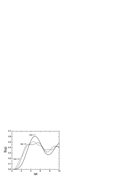
Figure 14: Variation of the ${\bar{S}(q)}$ structure factors for excitation of the lowest S${}_{\,tot}=1$ state of the rectangular spin tetramer with side length ratio $b/a$. This illustrates the use of powder structure factors in establishing the internal geometry of spin clusters. The dimer coupling is $\alpha=0.3$, however this only affects the overall normalization.

On converting these matrix elements to structure factors using Eqs.(12,14) we find different functional forms for each transition for both the single crystal and powder average results, as a result of the different weight factors and the three distinct ion pair separations. The powder average, unpolarized structure factors are

$${\bar{S}}^{\Psi_{0,1}\to\Psi_{1,n}}(q)=\hskip 113.81102pt$$

$$\begin{cases}\frac{(C_{0}+S_{0}/\sqrt{3})^{2}}{2}(1-j_{0}(qa)-j_{0}(qb)+j_{0}(qc)),&\text{n = 1}\\ \frac{(C_{0}+S_{0}/\sqrt{3})^{2}}{2}(1-j_{0}(qa)+j_{0}(qb)-j_{0}(qc)),&\text{n = 2}\\ \hskip 30.44466pt\frac{2}{3}\,S_{0}^{2}\,(1+j_{0}(qa)-j_{0}(qb)-j_{0}(qc)),&\text{n = 3}\end{cases}$$ (110)

where $c=\sqrt{a^{2}+b^{2}}$. In Fig.13 we show these structure factors for a case with moderate interdimer coupling $(\alpha=0.3)$ for a rectangle of side ratio $b/a=1.5$. The transition to the highest S${}_{\,tot}=1$ excited state $|\Psi_{1,3}\rangle$ is much weaker than the other two, and so is multiplied by a factor of 10 in the figure for visibility.

Note that the excitation of the highest S${}_{\,tot}=1$ state $|\Psi_{1,3}\rangle$, which is a doubly-excited dimer ($|\sigma\sigma\rangle$), is only possible because the ground state has an $O(\alpha)$ excited component, in addition to the dominant “bare” $|\rho\rho\rangle$ basis state. The weakness of the $|\Psi_{1,3}\rangle$ signal is because the structure factor is proportional to the nonleading ground state amplitude squared, so that it is $O(\alpha^{2})$. The observation of similar “non-valence state” transitions which are forbidden at $O(\alpha^{0})$ should allow direct experimental tests of the “interaction” terms in quantum spin Hamiltonians such as this one. The strength alone is a sensitive measure of $\alpha$, and the spatial modulation of $\bar{S}(q)$ is clearly different from the $O(\alpha^{0})$ transitions that dominate the structure factors of the lower-lying S${}_{\,tot}=1$ states.

The detailed $q$-dependence of the structure factors can be used as a “fingerprint” to test whether a given structure is indeed the magnetically active system. As an example, in Fig.14 we show that the detailed form of the structure factor to the first S${}_{\,tot}=1$ state shows significant variation with the ratio $b/a$. (Values of $b/a=$ 1, 2 and 4 are shown.) This type of dependence could be used to establish the geometry of a magnetic subsystem, or to check powder neutron scattering results against the geometry of a proposed spin system.

III.3.3 Linear Tetramer

The linear tetramer consists of two dimers with internal magnetic couplings of strength J, with a single interdimer coupling of strength $\alpha$J between the two adjacent end spins (see Fig.10). The term “linear” refers only to the pattern of magnetic couplings; the actual spatial geometry of our linear tetramer is not assumed to be a straight line. The “Clemson tetramer” NaCuAsO₄ Ulu03 is a recent example of a possible “linear tetramer” that does not have a true collinear dimer geometry.

The linear tetramer Hamiltonian matrix is also relatively simple in the dimer pair basis of Eqs.(A.8-A.10). The single S${}_{tot}=2$ basis state $|(\sigma\sigma)\rangle_{2}$ is diagonal, with energy

$$\rm E_{2}=\Big{(}\frac{1}{2}+\frac{1}{4}\alpha\Big{)}\,{\rm J}\ .$$ (111)

The S${}_{tot}=1$ basis state $|(\rho\sigma)_{A}\rangle$ is also diagonal, with energy

$$\rm E_{1,\,2}=-\Big{(}\frac{1}{2}-\frac{1}{4}\alpha\Big{)}\,{\rm J}\ .$$ (112)

The remaining S${}_{tot}=1$ and S${}_{tot}=0$ two-dimensional Hamiltonian matrices are

$${\cal H}_{\rm S_{tot}=1}=\frac{1}{2}\,{\rm J}\left[\begin{array}[]{cc}\ 1-\frac{1}{2}\alpha&\alpha\\ \alpha&\ -1-\frac{1}{2}\alpha\end{array}\right]$$ (113)

and

$${\cal H}_{\rm S_{tot}=0}=\frac{1}{2}\,{\rm J}\left[\begin{array}[]{cc}\ 1-\alpha&\frac{\sqrt{3}}{2}\alpha\\ \frac{\sqrt{3}}{2}\alpha&\ -3\end{array}\right]$$ (114)

with eigenvalues

$${\rm E}_{1,\{{1\atop 3}\}}=-\Big{(}\frac{1}{4}\alpha\pm\frac{1}{2}\sqrt{1+\alpha^{2}}\;\Big{)}\,{\rm J}$$ (115)

and

$${\rm E}_{0,\{{1\atop 2}\}}=-\Bigg{(}\frac{1}{2}+\frac{1}{4}\alpha\pm\sqrt{1-\frac{1}{2}\alpha+\frac{1}{4}\alpha^{2}}\;\Bigg{)}\;{\rm J}$$ (116)

respectively.

The susceptibility of the linear tetramer, which follows from these energy levels and Eq.(7), is given in Table LABEL:chi_table. As with the rectangular tetramer, the expression we find for the specific heat is too lengthly to tabulate here.

The neutron scattering structure factors from the linear tetramer S${}_{\,tot}=0$ ground state $|\Psi_{0,1}\rangle$ to the three S${}_{\,tot}=1$ excited states $|\Psi_{1,1\dots 3}\rangle$ may be calculated using the same techniques we applied to the rectangular tetramer. The results are somewhat more complicated, since two of the S${}_{\,tot}=1$ linear tetramer states are rotated between the dimer-pair basis states, in addition to the ground state basis rotation we found for the rectangular tetramer. The energy eigenvectors in these sectors are the superpositions of dimer-pair basis states given in Table LABEL:wavefunctions2, with mixing angles that satisfy

$$\tan(\theta_{1})=\frac{\alpha}{1+\sqrt{1+\alpha^{2}}}\ ,$$ (117)

$$\tan(\theta_{0})=\frac{\sqrt{3}\,\alpha/4}{1-\alpha/4+\sqrt{1-\alpha/2+\alpha^{2}/4}}\ .$$ (118)

This more complicated basis mixing pattern introduces a new feature, which is that the functional forms of the structure factors for the two mixed S${}_{\,tot}=1$ states, $|\Psi_{1,1}\rangle$ and $|\Psi_{1,3}\rangle$, depend on the dimer coupling $\alpha$. (In the rectangular tetramer system discussed previously we found that changing the dimer coupling $\alpha$ only changed the overall normalization of the structure factors, not their detailed $q$ dependence.)

We will give explicit results for the first transition, $|\Psi_{0,1}\rangle\to|\Psi_{1,1}\rangle$, and then simply quote the results for the two remaining final states. The matrix element of the neutron scattering transition operator $V_{a}$ is

$${}_{11}\langle\Psi_{1,1}|V_{+}|\Psi_{0,1}\rangle=c_{14}\,(f_{1}-f_{4})+c_{23}\,(f_{2}-f_{3})$$ (119)

where

$$\left\{\begin{array}[]{l}c_{14}\\ c_{23}\\ \end{array}\right\}=\pm\frac{(C_{0}+S_{0}/\sqrt{3})\,C_{1}}{2\sqrt{2}}+\frac{S_{0}S_{1}}{\sqrt{6}}$$ (120)

and $C_{0,1}$ and $S_{0,1}$ are respectively cos and sin of the linear tetramer basis state mixing angles, which were defined in Eqs.(117,118).

Figure 15: Powder average, unpolarized structure factors ${\bar{S}(q)}$ for the excitation of the three S${}_{\,tot}=1$ states of the linear tetramer, including the ionic form factor, with magnetic coupling ratio $\alpha=0.4$ and ion positions taken from the NaCuAsO₄ structure Ulu03 . The structure factor for the transition to the third state is scaled up by a factor of 10 for visibility.

The resulting unpolarized powder structure factor for this transition, using Eqs.(14,15), is

$${\bar{S}}^{\Psi_{0,1}\to\Psi_{1,1}}=\hskip 113.81102pt$$

$$2\Big{(}c_{14}^{\;2}\big{(}1-j_{0}(qr_{14})\big{)}+c_{23}^{\;2}\big{(}1-j_{0}(qr_{23})\big{)}$$

$$\hskip 28.45274pt+2\,c_{14}\,c_{23}\,(j_{0}(qr_{12})-j_{0}(qr_{13}))\Big{)}.$$ (121)

The transition from the ground state to the second linear tetramer S${}_{\,tot}=1$ excited state is given by a matrix element we encountered previously in the rectangular tetramer problem, except for a change in spatial geometry. The result for the unpolarized powder structure factor with completely general ion positions is

$${\bar{S}}^{\Psi_{0,1}\to\Psi_{1,2}}(q)=\hskip 113.81102pt$$

$$\frac{(C_{0}+S_{0}/\sqrt{3})^{2}}{2}\Big{(}1+\frac{1}{2}\big{(}-j_{0}(qr_{12})-j_{0}(qr_{13})+j_{0}(qr_{14})$$

$$+j_{0}(qr_{23})-j_{0}(qr_{24})-j_{0}(qr_{34})\big{)}\Big{)}.$$ (122)

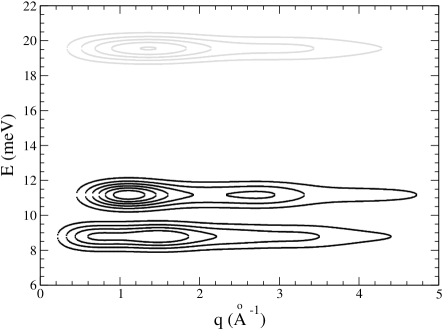
Figure 16: Contours of equal intensity of the powder average, unpolarized structure factors of the linear tetramer, with parameters appropriate to NaCuAsO₄, as in Fig.15. The contours are normalized to the peak of the first transition, and intervals of 0.2 in intensity are shown for the two lower states. The much weaker third transition is displayed with intervals of 0.01.

The structure factor for the third S${}_{\,tot}=1$ state $\Psi_{1,3}$ may be found from the $\Psi_{1,1}$ structure factor of Eq.(121) with the simple substitutions $(C_{1}\to S_{1}),(S_{1}\to-C_{1})$.

We will illustrate the predicted structure factors for the linear tetramer assuming parameters appropriate for the candidate material NaCuAsO₄ Ulu03 ; Nag03 . The ion pair separations are $r_{12}=r_{34}=3.641$ Å, $r_{13}=r_{24}=3.863$ Å  $r_{14}=6.814$ Å and $r_{23}=3.151$ Å. The copper positions are consistent with planarity, although our results do not require this assumption. There are indications of three S${}_{\,tot}=1$ levels in this material from a recent inelastic neutron scattering experiment, with energies of approximately 9, 11 and 18 meV Nag03 ; in the linear tetramer model this suggests parameters of J $\approx 10$ meV and $\alpha\approx 0.4$, which we will assume here. (The structure factors only depend on $\alpha$.) We also incorporated a simple Cu²⁺ ionic form factor, $F(q)=1/(1+q^{2}/q_{0}^{2})^{3}$ with $q_{0}=8.0$ Å^-1, which agrees with the online ILL Cu²⁺ form factor ILLsite to $\lesssim 0.5$ % over the range of $q$ shown. Our results are shown in Fig.15; characteristic features include the displaced relative maxima of the intensities of the two lower states, and the much weaker transition to the highest S${}_{\,tot}=1$ state. The results for the two lower states are rather insensitive to $\alpha$. The overall scale of the $|\Psi_{1,3}\rangle$ structure factor however is quite sensitive to $\alpha$, and scales approximately as $\alpha^{2}$. A measurement of the relative strength of these transitions would provide a useful determination if $\alpha$, which could be compared with the value extracted from the energy levels. (In principle the susceptibility could also be used to determine $\alpha$, but we have found that it has a rather weak $\alpha$ dependence in this system.)

In Fig.16 we show these results in a contour plot, approximately as would be observed in a neutron scattering experiment. (Our results should be multiplied by the energy-dependent factor $k^{\prime}/k$ of Eq.(11) for a direct comparison with experiment.) To generate this plot we have convolved a Gaussian energy resolution function, $\exp(-(E-E_{i})^{2}/2\sigma_{E}^{2})$ with $\sigma_{E}=0.5$ meV, with the structure factors to the three S${}_{tot}=1$ states. The intensities are shown relative to the maximum excitation intensity of the transition to the lowest S${}_{tot}=1$ state, $|\Psi_{0,1}\rangle\to|\Psi_{1,1}\rangle$. Note the characteristic strong peak in intensity of the second transition, $|\Psi_{0,1}\rangle\to|\Psi_{1,2}\rangle$, near $1.1$ Å^-1. Comparison of these general features with the data of Nagler et al. Nag03 suggests that the linear tetramer model does indeed give a realistic description of neutron scattering from NaCuAsO₄.

IV Future Applications

In the previous section we presented results for bulk thermodynamic and magnetic properties of various dimer, trimer and tetramer molecular magnets with S = 1/2 ions. We also derived the inelastic neutron scattering structure factors for these systems; inelastic neutron scattering is very useful as a local probe of magnetic interactions at the atomic scale. These results clearly have many possible applications to real materials. In this section we discuss some examples of materials that are thought to be realizations of S = 1/2 dimer, trimer and tetramer molecular magnets, and describe how our results could be useful in future experimental investigations. We also discuss possible extensions of this work, which will be useful in interpreting experimental data on these and related magnetic materials under more general circumstances.

The S = 1/2 spin dimer is the simplest of all spin clusters. It provides a textbook case for studies of finite spin systems more generally, since physical observables for the dimer can often be derived as closed form analytic expressions. This is the case for the specific heat, susceptibility and neutron scattering structure factors presented here. Vanadyl hydrogen phosphate, VO(HPO₄)$\cdot$0.5H₂O, is a well known example of an S = 1/2 spin dimer material Joh84 ; Ten97 ; Koo04 , and some of the results tabulated here have already been used in interpreting data on this material. In particular, the magnetic susceptibility was originally used to determine the exchange constant J, and inelastic neutron scattering was used to test the simple dimer model and establish which pair of V⁴⁺ ions forms the dimer Ten97 . This experiment was a dramatic success for inelastic neutron scattering, as the previously assumed V-V dimer pair was shown to have been misidentified.

Many examples of S=1/2 ion trimers have been reported in the literature. These systems are interesting in that the ground state is (ideally) degenerate, and must exhibit ferromagnetism. (S${}_{tot}>0$ for any energy eigenstate of an isotropic magnetic Hamiltonian with half-integer ion spins and an odd number of ions.) Heisenberg trimers with antiferromagnet pair interactions are also of interest because they are the simplest isotropic spin systems which experience frustration. One example of an S=1/2 trimer is Cu₃(O₂C₁₆H₂₃)${}_{6}\cdot 1.2$C₆H₁₂ Cag03a ; Cag03b , which has an equilateral Cu²⁺ triangle with a Cu²⁺ - Cu²⁺ separation of 3.131 Å. Recent Electron Paramagnetic Resonance (EPR) measurements show that the ground state of this material consists of a twofold-degenerate S${}_{tot}=1/2$ level; this is in accord with expectations for a general isotropic trimer antiferromagnet with S = 1/2 ions, but not with the perfect equilateral (symmetric) case, in which the ground state is a quartet of two degenerate S${}_{tot}=1/2$ levels. The gap to the S${}_{tot}=3/2$ excited level is estimated from both EPR and susceptibility data to be 28 meV Cag03a ; Cag03b . There are indications from the EPR studies that this fourfold degeneracy has been lifted by additional, nonisotropic interactions Cag03b . Investigation of the level structure and structure factors in this apparently symmetric trimer material would be a very interesting exercise for a future inelastic neutron scattering experiment, especially if large single crystals are available.

Another recent example of an S=1/2 trimer is the “Na₉-2” material of Kortz et al. Kor04 , Na₉[Cu₃Na₃(H₂O)₉ ($\alpha$-AsW₉O₃₃)₂]$\cdot$26H₂O, which contains an equilateral Cu${}^{2+}_{3}$ trimer with a susceptibility consistent with equal Heisenberg interactions of J $\approx 0.35$ meV. Inelastic neutron scattering from a powder sample of this material should show the S${}_{tot}=3/2$ excited level, with a structure factor proportional to $(1-j_{0}(qa))$. With a single crystal sample it might be possible to separate the transitions from the two (nearly?) degenerate S${}_{tot}=1/2$ levels to the S${}_{tot}=3/2$ excited level.

The two “V₆” materials of Luban et al. Lub02 , (CN₃H₆)₄ Na₂[H₄V₆O₈(PO₄)₄ ((OCH₂)₃ CCH₂OH)₂] $\cdot$14H₂O and Na₆[H₄V₆O₈(PO₄)₄ ((OCH₂)₃CCH₂OH)₂]$\cdot$18H₂O, contain pairs of (presumably weakly coupled) V₃ spin trimers that are respectively isosceles and general triangular systems. The isosceles V₆ material was used as an example of single-crystal inelastic neutron scattering structure factors in this paper.

The “V₁₅” material K₆[V₁₅As₆O₄₂(H₂O)]$\cdot$8H₂O is an example of an S=1/2 trimer in a more complicated magnetic geometry. This material has a frustrated V₃ triangle sandwiched between two nonplanar antiferromagnetic V₆ hexagons. The low-temperature magnetic properties are dominated by the V₃ triangle; other magnetic interactions become important at elevated temperatures Bar92 ; Mue88 ; Gat91 ; Cha02 ; Cha04 ; Cho03 . In addition to distinguishing between direct vanadium-vanadium and superexchange pathways involving the upper and lower hexagons, neutron scattering was used to probe the magnetic structure, finding two nearly degenerate S_tot = 1/2 ground states (with 0.035 meV splitting) and an S_tot = 3/2 excited state Cha02 . The availability of large single crystals of this material suggests that it might be an interesting candidate for inelastic neutron scattering studies.

Clearly, the analytical expressions we have presented here for spin-trimer thermodynamic properties and inelastic neutron scattering amplitudes have wide potential application, and should be useful in particular for interpreting the results of future inelastic neutron scattering experiments on spin-trimer molecular magnets.

Examples of tetramer systems with S = 1/2 ions include sodium copper arsenate, NaCuAsO₄ Ulu03 ; Nag03 , which we used as an illustration of the evaluation of inelastic neutron scattering structure factors in the previous section. The neutron scattering data of Nagler et al. Nag03 supports a model of this material as an open-chain tetramer, with antiferromagnetic Heisenberg bonds of alternating strength. Transitions from the S${}_{tot}=0$ ground state to all three S${}_{tot}=1$ triplet excited states have been observed on a powder sample Nag03 , and the relative intensities and the $q$-dependence of the powder average structure factors appear to be approximately consistent with our predictions for the open-chain model. As we have given detailed analytic predictions for the neutron structure factor for these transitions, a comparison with data from a high-statistics experiment on a larger powder sample should be straightforward.

Additional examples of S = 1/2 tetramers are found in vanadium materials containing the [V₁₂As₈O₄₀(H₂O)]^4- cluster anion. Basler et al. Bas02 have recently reported studies of the magnetic properties of three such materials, Na₄[V₁₂As₈O₄₀(H₂O)]$\cdot$23H₂O, Na₄[V₁₂As₈O₄₀(D₂O)] $\cdot$16.5D₂O and (NHEt₃)[V₁₂As₈O₄₀(H₂O)]$\cdot$H₂O. These materials have three stacked V₄ tetramers, but are mixed-valent (V${}^{4+}_{8}$V${}^{+5}_{4}$). The middle tetramer dominates the magnetic properties. This tetramer is anti- ferromagnetic and close to square, with exchange constants of $\approx 1.5$ meV (inferred from energy levels established by EPR and inelastic neutron scattering). The Basler et al. study is a very nice illustration of the combined use of bulk magnetic properties and inelastic neutron scattering to characterize magnetic materials, as we advocate in this work. Additional studies of this already well characterized material might involve an inelastic neutron scattering study of a single crystal, which could be used to test the detailed orientation dependence expected for the structure factor for each of the observed magnetic transitions to excited states, given their fitted magnetic Hamiltonian. Since this Hamiltonian includes anisotropies, a study using polarized neutrons could provide additional useful information.

There are several interesting questions which were not considered in detail in this paper that would be appropriate for future research on finite spin clusters. Consideration of higher ionic spin is one obvious generalization of this work. Several examples of uncompensated molecular magnets (which have ground states with nonzero spin) may be found in relatively simple higher-spin materials. One example is the first cobalt molecular magnet Yang , Co₄(NC₅H₄H₂CO)₄(CH₃OH)₄Cl₄. This material consists of four S = 3/2 Co²⁺ ions and four ligand-related oxygen atoms situated on the corners of a cube, with a ferromagnetic S${}_{tot}=6$ ground state. The magnetic exchange constants have been estimated from fits to magnetization curves, and are at the meV scale Yang . The magnetic Co²⁺ ions in this material form a tetramer with important tetrahedral and dimer magnetic interactions Yang , which would be an important case for future neutron scattering studies, especially with large single crystals. Another example of a molecular magnet with higher ion spin is the chromium magnet [Cr₄S(O₂CCH₃)₈(H₂O)₄](NO₃)₂^.H₂O, which has four ferromagnetically coupled S = 3/2 Cr³⁺ ions arranged in a nearly regular tetrahedron, with an S${}_{tot}=6$ ground state. Furukawa et al. Fur00 determined the exchange constant for this material from the susceptibility, and predict a gap to the first S${}_{tot}=5$ excited state of ca. 15 meV. Observation of this excitation using inelastic neutron scattering should be a straightforward exercise, and the intensities should agree well with theoretical expectations of the Heisenberg model, since this model gives a reasonably good description of the bulk magnetic properties.

Extension of this work to mixed-valent spin clusters would also be interesting, since many examples of these are known, including systems with magnetized ground states. One example is the “Mn₄” material [Mn₄O₃Cl₄(O₂CEt)₃(py)₃]${}_{2}\cdot 2$C₆H₁₄ studied by Hill $et~{}al.$ Hil03 , which has a mixed-valent spin tetramer consisting of a triangle of S = 2 Mn³⁺ ions with an apical S = 3/2 Mn⁴⁺, and a ground-state spin of S${}_{tot}=9/2$. Although the interest in this material as a molecular magnet is largely due to the weak coupling between pairs of Mn₄ clusters, the magnetic Hamiltonian within a single Mn₄ cluster could be tested by powder inelastic neutron scattering.

Another interesting theme for future studies is the effect of finite temperatures on inelastic neutron scattering; although increasing temperatures are usually associated with weaker inelastic transitions, the finite Hilbert space of a spin cluster implies that magnetic transitions will weaken in a simple, known manner according to their Boltzman factors, and will approach finite limits at high temperatures (provided that the magnetic Hamiltonian remains valid). Since moderate temperatures (on the scale of the magnetic excitations) will significantly populate excited levels, it may also be possible to observe inelastic transitions from excited levels that are inaccessible at low temperatures.

Another important topic which we briefly alluded to in the text is the issue of magnetic interactions between spin clusters; these interactions will broaden the discrete levels assumed here into bands, which will be observable if the intercluster interactions are sufficiently large.

Finally, the generalization of our results to non-Heisenberg interactions, and the determination of these interaction parameters through polarized inelastic neutron scattering experiments, would be an especially interesting and important extension of the work presented here.

V Summary and Conclusions

In this paper we have evaluated several thermodynamic and neutron scattering observables that characterize the magnetic behavior of finite quantum spin systems. After an introduction that gives results applicable to the general case, we specialized to clusters of S=1/2 ions with a Heisenberg interaction between ion pairs. We considered dimer, trimer and tetramer systems with various magnetic interaction strengths, and evaluated the magnetic specific heat, the susceptibility, and the inelastic neutron scattering structure factor for these systems. The structure factor was derived both for single crystals and for the powder average case. Our results for the neutron scattering structure factor show that accurate intensity measurements of inelastic neutron scattering cross sections from a powder can be useful in establishing the spatial geometry of an assumed set of interacting magnetic ions. The linear spin-tetramer candidate NaCuAsO₄ was considered as an example, and we found that the observed inelastic powder pattern for excitation of the two lowest S${}_{tot}=1$ excited levels is indeed consistent with the predictions of the linear tetramer model. We also considered inelastic neutron scattering from single crystals, and found dramatic angular dependence that could be used in future experiments as sensitive tests of the assumed magnetic Hamiltonian. We concluded with a discussion of specific materials that might be studied using our results, and suggested future extensions of our work to more general systems.

VI Acknowledgements

This project was supported by the Petroleum Research Fund administered by the American Chemical Society (PRF-AC 38164) and the Joint Institute for Neutron Sciences. TB also acknowledges support from the Neutron Sciences Consortium of the University of Tennessee. We are grateful to C.C.Torardi for providing a sample of the spin dimer VO(HPO₄)$\cdot$0.5H₂O, J.R.Thompson for measuring the susceptibility, and S.E.Nagler for useful communications and access to unpublished data on NaCuAsO₄.

APPENDIX: Tetramer basis states and matrix elements

Since there is a natural separation of the rectangle and linear tetramer systems into dimer components, it is useful to introduce a $|(12)(34)\rangle$ dimer basis to represent tetramer energy eigenvectors. The dimer basis states are

$$|\rho\rangle=\frac{1}{\sqrt{2}}\,\Big{(}|\!\uparrow\downarrow\,\rangle-|\!\downarrow\uparrow\,\rangle\Big{)}$$ (A.1)

and

$$|\sigma(m)\rangle=\left[\begin{array}[]{cl}|\!\uparrow\uparrow\,\rangle&m=+1\\ \\ \frac{1}{\sqrt{2}}\,\Big{(}|\!\uparrow\downarrow\,\rangle+|\!\downarrow\uparrow\,\rangle\Big{)}&m=0\\ \\ |\!\downarrow\downarrow\,\rangle&m=-1\\ \end{array}\right]_{\ .}$$ (A.7)

These are combined as Clebsch-Gordon series to form tetramer basis states of definite total spin and symmetry, which are $|(\sigma\sigma)_{S}\rangle,\,\rm S_{tot}=0,2$; $|(\sigma\sigma)_{A}\rangle,\,\rm S_{tot}=1$; $|(\rho\sigma)_{S,A}\rangle,\,\rm S_{tot}=1$; $|\rho\rho\rangle,\,\rm S_{tot}=0$. In the interest of clarity we will occasionally specify the total spin of one of these basis state with a subscript; thus $|\sigma\sigma\rangle_{0}$ refers to the $|(\sigma\sigma)_{S}\rangle$ state with $\rm S_{tot}=0$.

Using these states as basis vectors reduces the 16-dimensional full tetramer Hilbert space to 1-, 2- and 3-dimensional subspaces, which are spanned by the basis sets

$$\!|\;\rm S_{tot}=2\rangle\ \ \ \ =\ \ |\sigma\sigma\rangle_{2}\\$$ (A.8)

$$\qquad\!\{\;|\;\rm S_{tot}=1\rangle\;\}=\left[\begin{array}[]{c}|\sigma\sigma\rangle_{1}\\ \\ |(\rho\sigma)_{S}\rangle\\ \\ |(\rho\sigma)_{A}\rangle\\ \end{array}\right]$$ (A.9)

$$\quad\!\{\;|\;\rm S_{tot}=0\rangle\;\}\ =\left[\begin{array}[]{c}|\sigma\sigma\rangle_{0}\\ \\ |\rho\rho\rangle\\ \end{array}\right]_{\ .}$$ (A.10)

Thus symmetry arguments alone determine the eigenvectors for one level, and the eigenvectors for the remaining levels involve at most $2\times 2$ and $3\times 3$ diagonalizations. As we shall see, for the three tetramer models we consider here we actually encounter at most $2\times 2$ diagonalization problems using this basis.

These basis states are also convenient for determining neutron scattering structure factors, since they have relatively simple matrix elements of the spin transition operator $V_{a}$ of Eq.(10). The complete set of matrix elements of $V_{a}$ (spherical components) between single (12)-dimer basis states, with $f_{i}=e^{i\vec{k}\cdot\vec{x}_{i}}$, is

$$\langle\rho\,|\,V_{a}\,|\rho\rangle=0$$ (A.11)

$$\langle\sigma(m)\,|\,V_{a}\,|\rho\rangle=\delta_{a,m}\frac{f_{1}-f_{2}}{2}$$ (A.12)

$$\langle\rho\,|\,V_{a}\,|\sigma(m)\rangle=-\delta_{a,-m}\frac{f_{1}-f_{2}}{2}$$ (A.13)

$$\langle\sigma(m^{\prime})|\,V_{a}\,|\sigma(m)\rangle=-\delta_{m^{\prime},m+a}\frac{f_{1}+f_{2}}{2}\ .$$ (A.14)

These dimer results may be combined to give the complete set of matrix elements of $V_{a}$ between tetramer basis states, which is all that we require to determine all neutron scattering structure factors for all the spin tetramer problems we consider. These tetramer matrix elements (with explicit S${}_{\,tot}$ or S${}_{\,tot}$, S${}_{z\,tot}$ subscripts on the states where required for clarity) are

$$\phantom{{}_{1,m}}\langle\rho\rho\,|\,V_{a}\,|\rho\rho\rangle=0\hskip 142.26378pt$$ (A.15)

$${}_{1,m}\langle(\rho\sigma)_{S}\,|\,V_{a}\,|\rho\rho\rangle=$$

$$\hskip 85.35826pt\delta_{a,m}\frac{f_{1}-f_{2}+f_{3}-f_{4}}{2\sqrt{2}}$$ (A.16)

$${}_{1,m}\langle(\rho\sigma)_{A}\,|\,V_{a}\,|\rho\rho\rangle=$$

$$\hskip 85.35826pt\delta_{a,m}\frac{f_{1}-f_{2}-f_{3}+f_{4}}{2\sqrt{2}}$$ (A.17)

$$\phantom{{}_{1,m}}\langle\sigma\sigma\,|\,V_{a}\,|\rho\rho\rangle=0\hskip 142.26378pt$$ (A.18)

$$\phantom{{}_{1,m}}\langle\rho\rho\,|\,V_{a}\,|\sigma\sigma\rangle=0\hskip 142.26378pt$$ (A.19)

$${}_{1,m}\langle(\rho\sigma)_{S}\,|\,V_{a}\,|\sigma\sigma\rangle_{0}=$$

$$\hskip 85.35826pt-\delta_{a,m}\frac{f_{1}-f_{2}+f_{3}-f_{4}}{2\sqrt{6}}$$ (A.20)

$${}_{1,m}\langle(\rho\sigma)_{A}\,|\,V_{a}\,|\sigma\sigma\rangle_{0}=$$

$$\hskip 85.35826pt-\delta_{a,m}\frac{f_{1}-f_{2}-f_{3}+f_{4}}{2\sqrt{6}}$$ (A.21)

$${}_{\phantom{,m}0}\langle\sigma\sigma\,|\,V_{a}\,|\sigma\sigma\rangle_{0}=0$$ (A.22)

$${}_{1,m}\langle\sigma\sigma\,|\,V_{a}\,|\sigma\sigma\rangle_{0}=$$

$$\hskip 85.35826pt\delta_{a,m}\frac{f_{1}+f_{2}-f_{3}-f_{4}}{\sqrt{6}}$$ (A.23)

$${}_{\phantom{,m}2}\langle\sigma\sigma\,|\,V_{a}\,|\sigma\sigma\rangle_{0}=0$$ (A.24)

The remaining matrix elements between pairs of S_tot $=$ $1$ states and between S${}_{tot}=1$ and S${}_{tot}=2$ states, which were not required in this paper, may be evaluated similarly.

Table 2: Energy eigenvectors and eigenvalues.

Spin System	Eigenvector $|\Psi_{\rm S_{tot}}\rangle$ (S${}_{z\,tot}=$ S${}_{\,tot}$)	Energy
Dimer	$|\Psi_{1}\rangle=|\sigma(+1)\rangle=|\!\uparrow\uparrow\,\rangle$	E${}_{1}=\phantom{-}\frac{1}{4}\,{\rm J}$
	$|\Psi_{0}\rangle=|\rho\rangle=\quad\frac{1}{\sqrt{2}}(|\!\uparrow\downarrow\,\rangle-|\!\downarrow\uparrow\,\rangle)$	E${}_{0}=-\frac{3}{4}\,{\rm J}$
Symmetric Trimer	$|\Psi_{\frac{3}{2}}\rangle\ =\;|\sigma(+3/2)\rangle=|\!\uparrow\uparrow\uparrow\,\rangle$	E${}_{\frac{3}{2}}=\phantom{-}\frac{3}{4}\,{\rm J}$
	$|\Psi_{\frac{1}{2},2}\rangle=|\lambda(+1/2)\rangle=\frac{1}{\sqrt{6}}(|\!\uparrow\downarrow\uparrow\,\rangle+|\!\downarrow\uparrow\uparrow\,\rangle-2|\!\uparrow\uparrow\downarrow\,\rangle)$	E${}_{\frac{1}{2}}=-\frac{3}{4}\,{\rm J}$
	$|\Psi_{\frac{1}{2},1}\rangle=|\rho(+1/2)\rangle=\frac{1}{\sqrt{2}}(|\!\uparrow\downarrow\uparrow\,\rangle-|\!\downarrow\uparrow\uparrow\,\rangle)$
Isosceles Trimer	$|\Psi_{\frac{3}{2}}\rangle\ =\;|\sigma(+3/2)\rangle$	E${}_{\frac{3}{2}}=(\frac{1}{4}+\frac{1}{2}\alpha)\,{\rm J}$
	$|\Psi_{\frac{1}{2},2}\rangle=|\lambda(+1/2)\rangle$	E${}_{\frac{1}{2},2}=(\frac{1}{4}-\alpha)\,{\rm J}$
	$|\Psi_{\frac{1}{2},1}\rangle=|\rho(+1/2)\rangle$	E${}_{\frac{1}{2},1}=-\frac{3}{4}\,{\rm J}$
General Trimer	$|\Psi_{\frac{3}{2}}\rangle\ =\;|\sigma(+3/2)\rangle$	E${}_{\frac{3}{2}}\ =\frac{1}{4}(1+\alpha_{s})\,{\rm J}$
	$|\Psi_{\frac{1}{2},2}\rangle=+\cos(\theta)|\lambda(+1/2)\rangle+\sin(\theta)|\rho(+1/2)\rangle$	E${}_{\frac{1}{2},2}=\frac{1}{4}(+\sqrt{(2-\alpha_{s})^{2}+3\,\alpha_{d}^{2}}\,-1-\alpha_{s})\,{\rm J}$
	$|\Psi_{\frac{1}{2},1}\rangle=-\sin(\theta)|\lambda(+1/2)\rangle+\cos(\theta)|\rho(+1/2)\rangle$	E${}_{\frac{1}{2},1}=\frac{1}{4}(-\sqrt{(2-\alpha_{s})^{2}+3\,\alpha_{d}^{2}}\,-1-\alpha_{s})\,{\rm J}$
Tetrahedron	$|\Psi_{2}\rangle=|\sigma\sigma\rangle_{2}\ =|\!\uparrow\uparrow\uparrow\uparrow\,\rangle$	E${}_{2}=\phantom{-}\frac{3}{2}\,{\rm J}$
	$|\Psi_{1,3}\rangle=|\sigma\sigma\rangle_{1}$	E${}_{1}=-\frac{1}{2}\,{\rm J}$
	$|\Psi_{1,2}\rangle=|(\rho\sigma)_{S}\rangle$
	$|\Psi_{1,1}\rangle=|(\rho\sigma)_{A}\rangle$
	$|\Psi_{0,2}\rangle=|\sigma\sigma\rangle_{0}$	E${}_{0}=-\frac{3}{2}\,{\rm J}$
	$|\Psi_{0,1}\rangle=|\rho\rho\rangle$
Rectangular tetramer	$|\Psi_{2}\rangle\ =\ |\sigma\sigma\rangle_{2}$	E${}_{2}=(\frac{1}{2}+\frac{1}{2}\alpha)\,{\rm J}$
	$|\Psi_{1,3}\rangle=|\sigma\sigma\rangle_{1}$	E${}_{1,3}=(\frac{1}{2}-\frac{1}{2}\alpha)\,{\rm J}$
	$|\Psi_{1,2}\rangle=|(\rho\sigma)_{S}\rangle$	E${}_{1,2}=(-\frac{1}{2}+\frac{1}{2}\alpha)\,{\rm J}$
	$|\Psi_{1,1}\rangle=|(\rho\sigma)_{A}\rangle$	E${}_{1,1}=(-\frac{1}{2}-\frac{1}{2}\alpha)\,{\rm J}$
	$|\Psi_{0,2}\rangle=+\cos(\theta_{0})|\sigma\sigma\rangle_{0}+\sin(\theta_{0})|\rho\rho\rangle$	E${}_{0,2}=(+\sqrt{1-\alpha+\alpha^{2}}-\frac{1}{2}-\frac{1}{2}\alpha)\,{\rm J}$
	$|\Psi_{0,1}\rangle=-\sin(\theta_{0})|\sigma\sigma\rangle_{0}+\cos(\theta_{0})|\rho\rho\rangle$	E${}_{0,1}=(-\sqrt{1-\alpha+\alpha^{2}}-\frac{1}{2}-\frac{1}{2}\alpha)\,{\rm J}$

Table 2: Energy eigenvectors and eigenvalues (cont).

Spin System	Eigenvector $|\Psi_{\rm S_{tot}}\rangle$ (S${}_{z\,tot}=$ S${}_{\,tot}$)	Energy
Linear Tetramer	$|\Psi_{2}\rangle\ \ =\ |\sigma\sigma\rangle_{2}$	E${}_{2}=(\frac{1}{2}+\frac{1}{4}\alpha)\,{\rm J}$
	$|\Psi_{1,3}\rangle=+\cos(\theta_{1})|\sigma\sigma\rangle_{1}+\sin(\theta_{1})|(\rho\sigma)_{S}\rangle$	E${}_{1,3}=(+\frac{1}{2}\sqrt{1+\alpha^{2}}-\frac{1}{4}\alpha)\,{\rm J}$
	$|\Psi_{1,2}\rangle=|(\rho\sigma)_{A}\rangle$	E${}_{1,2}=(-\frac{1}{2}+\frac{1}{4}\alpha)\,{\rm J}$
	$|\Psi_{1,1}\rangle=-\sin(\theta_{1})|\sigma\sigma\rangle_{1}+\cos(\theta_{1})|(\rho\sigma)_{S}\rangle$	E${}_{1,1}=(-\frac{1}{2}\sqrt{1+\alpha^{2}}-\frac{1}{4}\alpha)\,{\rm J}$
	$|\Psi_{0,2}\rangle=+\cos(\theta_{0})|\sigma\sigma\rangle_{0}+\sin(\theta_{0})|\rho\rho\rangle$	E${}_{0,2}=(+\sqrt{1-\frac{1}{2}\alpha+\frac{1}{4}\alpha^{2}}-\frac{1}{2}-\frac{1}{4}\alpha)\,{\rm J}$
	$|\Psi_{0,1}\rangle=-\sin(\theta_{0})|\sigma\sigma\rangle_{0}+\cos(\theta_{0})|\rho\rho\rangle$	E${}_{0,1}=(-\sqrt{1-\frac{1}{2}\alpha+\frac{1}{4}\alpha^{2}}-\frac{1}{2}-\frac{1}{4}\alpha)\,{\rm J}$

Table 3: Inelastic Neutron Scattering Transitions^a

System		Transition	$\Delta E$
Dimer	I.	$|\Psi_{0}\rangle\to|\Psi_{1}\rangle$	$\rm J$
Symmetric Trimer	I.	$|\Psi_{\frac{1}{2},1}\rangle\to|\Psi_{\frac{3}{2}}\rangle$	$\frac{3}{2}\,\rm J$
	II.	$|\Psi_{\frac{1}{2},2}\rangle\to|\Psi_{\frac{3}{2}}\rangle$
Isosceles Trimer	I.	$|\Psi_{\frac{1}{2},1}\rangle\to|\Psi_{\frac{3}{2}}\rangle$	$(1+\frac{1}{2}\alpha)\,\rm J$
	II.	$|\Psi_{\frac{1}{2},2}\rangle\to|\Psi_{\frac{3}{2}}\rangle$	$\frac{3}{2}\alpha\,\rm J$
	III.	$|\Psi_{\frac{1}{2},1}\rangle\to|\Psi_{\frac{1}{2},2}\rangle$	$(1-\alpha)\,\rm J$
General Trimer	I.	$|\Psi_{\frac{1}{2},1}\rangle\to|\Psi_{\frac{3}{2}}\rangle$	$(\frac{1}{2}(1+\alpha_{s})+\frac{1}{4}f_{0})\,\rm J$
	II.	$|\Psi_{\frac{1}{2},2}\rangle\to|\Psi_{\frac{3}{2}}\rangle$	$(\frac{1}{2}(1+\alpha_{s})-\frac{1}{4}f_{0})\,\rm J$
	III.	$|\Psi_{\frac{1}{2},1}\rangle\to|\Psi_{\frac{1}{2},2}\rangle$	$\frac{1}{2}f_{0}\,\rm J$
Tetrahedron	I.	$|\Psi_{0,1}\rangle\to|\Psi_{1,1}\rangle$	$\rm J$
	II.	$|\Psi_{0,1}\rangle\to|\Psi_{1,2}\rangle$
	III.	$|\Psi_{0,1}\rangle\to|\Psi_{1,3}\rangle$
	IV.	$|\Psi_{0,2}\rangle\to|\Psi_{1,1}\rangle$
	V.	$|\Psi_{0,2}\rangle\to|\Psi_{1,2}\rangle$
	VI.	$|\Psi_{0,2}\rangle\to|\Psi_{1,3}\rangle$
	VII.	$|\Psi_{1,1}\rangle\to|\Psi_{2}\rangle$	$2\rm J$
	VIII.	$|\Psi_{1,2}\rangle\to|\Psi_{2}\rangle$
	IX.	$|\Psi_{1,3}\rangle\to|\Psi_{2}\rangle$
Rectangular Tetramer	I.	$|\Psi_{0,1}\rangle\to|\Psi_{1,1}\rangle$	$f_{1}\,\rm J$
	II.	$|\Psi_{0,1}\rangle\to|\Psi_{1,2}\rangle$	$(f_{1}+\alpha)\,\rm J$
	III.	$|\Psi_{0,1}\rangle\to|\Psi_{1,3}\rangle$	$(f_{1}+1)\,\rm J$
	IV.	$|\Psi_{1,1}\rangle\to|\Psi_{0,2}\rangle$	$f_{1}\,\rm J$
	V.	$|\Psi_{1,1}\rangle\to|\Psi_{1,2}\rangle$	$\alpha\,\rm J$
	VI.	$|\Psi_{1,1}\rangle\to|\Psi_{1,3}\rangle$	$\rm J$
	VII.	$|\Psi_{1,1}\rangle\to|\Psi_{2}\rangle$	$(1+\alpha)\,\rm J$
	VIII.	$|\Psi_{1,2}\rangle\to|\Psi_{0,2}\rangle$	$(f_{1}-\alpha)\,\rm J$
	IX.	$|\Psi_{1,2}\rangle\to|\Psi_{1,3}\rangle$	$(1-\alpha)\,\rm J$
	X.	$|\Psi_{1,2}\rangle\to|\Psi_{2}\rangle$	$\rm J$
	XI.	$|\Psi_{0,2}\rangle\to|\Psi_{1,3}\rangle$	$(1-f_{1})\,\rm J$
	XII.	$|\Psi_{1,3}\rangle\to|\Psi_{2}\rangle$	$\alpha\,\rm J$
Linear Tetramer	I.	$|\Psi_{0,1}\rangle\to|\Psi_{1,1}\rangle$	$(f_{2}-\frac{1}{2}(f_{3}-1))\,\rm J$
	II.	$|\Psi_{0,1}\rangle\to|\Psi_{1,2}\rangle$	$(f_{2}+\frac{1}{2}\alpha)\,\rm J$
	III.	$|\Psi_{0,1}\rangle\to|\Psi_{1,3}\rangle$	$(f_{2}+\frac{1}{2}(f_{3}+1))\,\rm J$
	IV.	$|\Psi_{1,1}\rangle\to|\Psi_{0,2}\rangle$	$(f_{2}+\frac{1}{2}(f_{3}-1))\,\rm J$
	V.	$|\Psi_{1,1}\rangle\to|\Psi_{1,2}\rangle$	$\frac{1}{2}(f_{3}-1+\alpha)\,\rm J$
	VI.	$|\Psi_{1,1}\rangle\to|\Psi_{1,3}\rangle$	$f_{3}\,\rm J$
	VII.	$|\Psi_{1,1}\rangle\to|\Psi_{2}\rangle$	$\frac{1}{2}(f_{3}+1+\alpha)\,\rm J$
	VIII.	$|\Psi_{1,2}\rangle\to|\Psi_{0,2}\rangle$	$(f_{2}-\frac{1}{2}\alpha)\,\rm J$
	IX.	$|\Psi_{1,2}\rangle\to|\Psi_{1,3}\rangle$	$\frac{1}{2}(f_{3}+1-\alpha)\,\rm J$
	X.	$|\Psi_{1,2}\rangle\to|\Psi_{2}\rangle$	$\rm J$
	XI.	$|\Psi_{0,2}\rangle\to|\Psi_{1,3}\rangle$	$(-f_{2}+\frac{1}{2}(f_{3}+1))\,\rm J$
	XII.	$|\Psi_{1,3}\rangle\to|\Psi_{2}\rangle$	$\frac{1}{2}(-f_{3}+1+\alpha)\,\rm J$

This table uses the abbreviations $f_{0}=\sqrt{(2-\alpha_{s})^{2}+3\alpha_{d}^{2}}$, $f_{1}=\sqrt{1-\alpha+\alpha^{2}}$, $f_{2}=\sqrt{1-\alpha/2+\alpha^{2}/4}$, $f_{3}=\sqrt{1+\alpha^{2}}$.

Table 4: Specific Heats^a

Spin System	$C/k_{B}$
Dimer	$3(\beta{\rm J})^{2}e^{\beta{\rm J}}/(3+e^{\beta{\rm J}})^{2}$
Symmetric Trimer	$\frac{9}{4}(\beta{\rm J})^{2}e^{\frac{3}{2}\beta{\rm J}}/\big{(}1+e^{\frac{3}{2}\beta{\rm J}}\big{)}^{2}$
Isosceles Trimer	$\frac{1}{2}(\beta{\rm J})^{2}\Big{(}2(1-\alpha)^{2}e^{(1+2\alpha)\beta{\rm J}}+(2+\alpha)^{2}e^{(1+\frac{1}{2}\alpha)\beta{\rm J}}+9\alpha^{2}e^{\frac{3}{2}\alpha\beta{\rm J}}\Big{)}/\Big{(}2+e^{\frac{3}{2}\alpha\beta{\rm J}}+e^{(1+\frac{1}{2}\alpha)\beta{\rm J}}\Big{)}^{2}$
General Trimer	$\frac{1}{16}(\beta{\rm J})^{2}e^{\frac{1}{2}(1+\alpha_{s})\beta{\rm J}}\Big{(}f_{0}^{2}e^{\frac{1}{2}(1+\alpha_{s})\beta{\rm J}}+\big{(}4(1+\alpha_{s})^{2}+f_{0}^{2}\big{)}\cosh(f_{0}\beta{\rm J}/4)+4f_{0}(1+\alpha_{s})\sinh(f_{0}\beta{\rm J}/4)\Big{)}/$
	$\Big{(}1+e^{\frac{1}{2}(1+\alpha_{s})\beta{\rm J}}\cosh(f_{0}\beta{\rm J}/4)\Big{)}^{2}$
Tetrahedron	$18(\beta{\rm J})^{2}\Big{(}10e^{2\beta{\rm J}}+5e^{3\beta{\rm J}}+e^{5\beta{\rm J}}\Big{)}/\Big{(}5+9e^{2\beta{\rm J}}+2e^{3\beta{\rm J}}\Big{)}^{2}$

This table uses the abbreviation $f_{0}=\sqrt{(2-\alpha_{s})^{2}+3\alpha_{d}^{2}}$.

Table 5: Susceptibilities^a

Spin System	$\chi/(g\mu_{B})^{2}$
Dimer	$2\beta/\big{(}3+e^{\beta{\rm J}}\big{)}$
Symmetric Trimer	$\frac{1}{4}\beta\big{(}5+e^{\frac{3}{2}\beta{\rm J}}\big{)}/\big{(}1+e^{\frac{3}{2}\beta{\rm J}}\big{)}$
Isosceles Trimer	$\frac{1}{4}\beta{\Big{(}10+e^{\frac{3}{2}\alpha\beta{\rm J}}+e^{(1+\frac{1}{2}\alpha)\beta{\rm J}}\Big{)}}/{\Big{(}2+e^{\frac{3}{2}\alpha\beta{\rm J}}+e^{(1+\frac{1}{2}\alpha)\beta{\rm J}}\Big{)}}$
General Trimer	$\frac{1}{4}\beta{\Big{(}5+e^{\frac{1}{2}(1+\alpha_{s})\beta{\rm J}}\cosh(f_{0}\beta{\rm J}/4)\Big{)}}/{\Big{(}1+e^{\frac{1}{2}(1+\alpha_{s})\beta{\rm J}}\cosh(f_{0}\beta{\rm J}/4)\Big{)}}$
Tetrahedron	$2\beta\Big{(}5+3e^{2\beta{\rm J}}\Big{)}/\Big{(}5+9e^{2\beta{\rm J}}+2e^{3\beta{\rm J}}\Big{)}$
Rectangular Tetramer	$2\beta\Big{(}5+e^{\beta{\rm J}}+e^{\alpha\beta{\rm J}}+e^{(1+\alpha)\beta{\rm J}}\Big{)}/\Big{(}5+3e^{\beta{\rm J}}+3e^{\alpha\beta{\rm J}}+3e^{(1+\alpha)\beta{\rm J}}+2e^{(1+\alpha)\beta{\rm J}}\cosh(f_{1}\beta{\rm J}/2)\Big{)}$
Linear Tetramer	$2\beta\Big{(}5+e^{\beta{\rm J}}+2e^{\frac{1}{2}(1+\alpha)\beta{\rm J}}\cosh(f_{3}\beta{\rm J}/2)\Big{)}/$
	$\Big{(}5+3e^{\beta{\rm J}}+2e^{(1+\frac{1}{2}\alpha)\beta{\rm J}}\cosh(f_{2}\beta{\rm J})+6e^{\frac{1}{2}(1+\alpha)\beta{\rm J}}\cosh(f_{3}\beta{\rm J}/2)\Big{)}$

This table uses the abbreviations $f_{0}=\sqrt{(2-\alpha_{s})^{2}+3\alpha_{d}^{2}}$, $f_{1}=\sqrt{1-\alpha+\alpha^{2}}$, $f_{2}=\sqrt{1-\alpha/2+\alpha^{2}/4}$, $f_{3}=\sqrt{1+\alpha^{2}}$.

References

- (1) E.Dagotto and T.M.Rice, Science 271, 618 (1996).
- (2) A.L.Barra, A.Caneschi, A.Cornia, F.Frabrizi de Biani, D.Gatteschi, C.Sangregorio, R.Sessoli and L.Sorace, J. Am. Chem. Soc. 121, 5302 (1999).
- (3) D.P.DiVincenzo and D.Loss, J. Magn. Magn. Mater. 200, 202 (1999).
- (4) M.A.Nielsen and I.L.Chuang, Quantum Computation and Quantum Information (Cambridge, 2000).
- (5) Y.Furukawa, M.Luban, F.Borsa, D.C.Johnston, A.V.Mahajan, L.L.Miller, D.Mentrup, J.Schnack and A.Bino, Phys. Rev. B61, 8635 (2000).
- (6) A.Bouwen, A.Caneschi, D.Gatteschi, E.Goovaerts, D.Schoemaker, L.Sorace and M.Stefan, J. Phys. Chem. B105, 2658 (2001).
- (7) A.Cornia, R.Sessoli, L.Sorace, D.Gatteschi, A.L.Barra and C.Daiguebonne, Phys. Rev. Lett. 89, 257201 (2002).
- (8) D.Mentrup, J.Schnack and M.Luban, Physica A272, 153 (1999).
- (9) D.Mentrup, H.-J.Schmidt, J.Schnack and M.Luban, Physica A278, 214 (2000).
- (10) O.Cifta, J. Phys. A, 34, 1611 (2001).
- (11) J.W.Johnson, D.C.Johnston, A.J.Jacobson and J.F.Brody, J. Am. Chem. Soc. 106, 8123 (1984).
- (12) D.A.Tennant, S.E.Nagler, A.W.Garrett, T.Barnes and C.C.Torardi, Phys. Rev. Lett. 78, 4998 (1997).
- (13) H.-J.Koo, M.-H.Whangbo, P.D.verNooy, C.C.Torardi and W.J.Marshall, Inorg. Chem. 41, 4664 (2002).
- (14) M.Luban, F.Borsa, S.Bud’ko, P.Canfield, S.Jun, J.K.Jung, P.Kögerler, D.Mentrup, A.Müller, R.Modler, D.Procissi, B.J.Suh and M.Torikachvili, Phys. Rev. B66, 054407 (2002).
- (15) Y.Qiu, C.Broholm, S.Ishiwata, M.Azuma, M.Takano, R.Bewley and W.J.L.Buyers, arXiv:cond-mat/0205018.
- (16) B.Cage, F.A.Cotton, N.S.Dalal, E.A.Hillard, B.Ravkin and C.M.Ramsey, J. Am. Chem. Soc. 125, 5270 (2003).
- (17) B.Cage, F.A.Cotton, N.S.Dalal, E.A.Hillard, B.Ravkin and C.M.Ramsey, C. R. Chemie 6, 39 (2003).
- (18) U.Kortz, S.Nellutla, A.C.Stowe, N.S.Dalal, J.van Tol and B.S.Bassil, Inorg. Chem. 43, 144 (2004).
- (19) D.Procissi, A.Shastri, I.Rousochatzakis, M.AlRifai, P.Kögerler, M.Luban, B.J.Suh and F.Borsa, Phys. Rev. B69, 094436 (2004).
- (20) C.Gros, P.Lemmens, M.Vojta, R.Valentí, K.Y.Choi, H.Kageyama, Z.Hiroi, N.V.Mushnikov, T.Goto, M.Johnsson and P.Millet, Phys. Rev. B67, 174405 (2003).
- (21) J.Jensen, P.Lemmes and C.Gros, Europhys. Lett. 64, 689 (2003).
- (22) O.Kahn, Molecular Magnetism (VCH Publishers, New York, 1993).
- (23) M.H. Whangbo, H.J. Koo, and D. Dai, J. Solid State Chem. 176, 417 (2003).
- (24) M.Ameduri and R.A.Klemm, Phys. Rev. B66, 224404 (2002).
- (25) D.V.Efremov and R.A.Klemm, Phys. Rev. B66, 174427 (2002).
- (26) R.A.Klemm and M.Ameduri, Phys. Rev. B66, 012403 (2002).
- (27) O.Waldmann, Phys. Rev. B68, 174406 (2003).
- (28) M. Ulutagay-Kartin, S.-J Hwu and J.A.Clayhold, Inorgan. Chem. 42, 2405 (2003).
- (29) S.E.Nagler, G.E.Granroth, J.A.Clayhold, S.-J.Hwu, M.Ulutagay-Kartin, D.A.Tennant and D.T.Adroja (unpublished).
- (30) G.L.Squires, Introduction to the Theory of Thermal Neutron Scattering (Dover, 1996).
- (31) H.López-Sandoval, R.Contreras, A.Escuer, R.Vicente, S.Bernès, H.Nöth, G.J.Leigh and N.Barba-Behrens, J. Chem. Soc., Dalton Trans. 2648 (2002).
- (32) A.Müller and J.Döring, J. Angew. Chem., Int. Ed. Engl. 27, 1721 (1988).
- (33) A.L.Barra, D.Gatteschi, L.Pardi, A.Müller and J.Döring, J. Am. Chem. Soc. 114, 8509 (1992).
- (34) D.Gatteschi, L.Pardi, A.L.Barra, A.Müller and J.Döring, Nature, 354, 463 (1991).
- (35) G.Chaboussant, R.Basler, A.Sieber, S.T.Ochsenbein, A.Desmedt, R.E.Lechner, M.T.F.Telling, P.Kögerler, A.Müller and H.-U.Güdel, Europhys. Lett. 59, 291 (2002).
- (36) G.Chaboussant, S.T.Ochsenbein, A.Sieber, H.-U.Güdel, H.Mutka, A.Müller and B.Barbara, arXiv:cond-mat/0401614.
- (37) R.Basler, G.Chaboussant, A.Sieber, H.Andres, M.Murrie, P.Kögerler, H.Bögge, D.C.Crans, E.Krickemeyer, S.Janssen, H.Mutka, A.Müller and H.-U.Güdel, Inorg. Chem. 41, 5675 (2002).
- (38) B.Bleaney and K.D.Bowers, Proc. R. Soc. London, Ser.A, A214, 451 (1952).
- (39) J.R.Thompson and C.C.Torardi (unpublished).
- (40) R.Veit, J.-J.Girerd, O.Kahn, F.Robert and Y.Jeannin, Inorgan. Chem. 25, 4175 (1986).
- (41) The approximate analytic Cu2+ form factor we fitted is given at the URL http://www.ill.fr/dif/ccsl/ffacts/ ffactnode3.html and http://www.ill.fr/dif/ccsl/ffacts/ ffactnode5.html.
- (42) J.Choi, L.A.W.Sanderson, J.L.Musfeldt, A.Ellern and P.Kögerler, Phys. Rev. B68, 064412 (2003).
- (43) E.-C.Yang, D.N.Hendrickson, W.Wernsdorfer, M.Nakano, R.Sommer, A.L.Rheingold, M.Ledezma-Gairaud and G.Christou, J. Appl. Phys. 91, 7382 (2002).
- (44) S.Hill, R.S.Edwards, N.Aliaga-Alcalde and G.Christou, Science 302, 1015 (2003).