Collective Spin Dynamics in the ”Coherence Window” for Quantum Nanomagnets

Abstract

The spin coherence phenomena and the possibility of their observation in nanomagnetic insulators attract more and more attention in the last several years. Recently it has been shown that in these systems in large transverse magnetic field there can be a fairly narrow ”coherence window” for phonon and nuclear spin-mediated decoherence. What kind of spin dynamics can then be expected in this window in a crystal of magnetic nanomolecules coupled to phonons, to nuclear spin bath and to each other via dipole-dipole interactions? Studying multispin correlations, we determine the region of parameters where ”coherent clusters” of collective spin excitations can appear. Although two particular systems, namely crystals of $Fe_{8}$-triazacyclonane and $Mn_{12}$-acetate molecules, are used in this work to illustrate the results, here we are not trying to predict an existence of collective coherent dynamics in some particular system. Instead, we discuss the way how any crystalline system of dipole-dipole coupled nanomolecules can be analyzed to decide whether this system is suitable for attempts to observe coherent dynamics. The presented analysis can be useful in the search for magnetic systems showing the spin coherence phenomena.

I Introduction

In the last decade the quantum tunneling phenomenon in nanomagnetic insulators has been attracting extensive interest. Many experiments have been done to study the tunneling relaxation in the ensembles of magnetic molecules with central molecular spins $\vec{S}_{i}$. can00 ; BB00 ; WWrev ; TB These molecules couple to each other via dipole-dipole interactions, PSPRL ; VillSurf ; FernRelax ; TSDIP to phonons POL96 ; LuisBart ; LossLeu ; Pohjola ; TB and to nuclear spins. PSPRL ; PS96 ; PSSB The early study of these systems in a low temperature regime has been concentrated mainly on the incoherent tunneling in low transverse fields, when the magnitude of the ground state tunneling splitting $2\Delta_{o}$ (produced by the tunneling between two potential wells separated by a barrier of magnetic anisotropy; $\Delta_{o}$ is the tunneling matrix element) is small in comparison with the parameters describing interactions with environment providing anomalously high decoherence. During last several years more attention has been paid to the spin coherence phenomena. SpinPrec ; AepSci ; LossCoh ; Kent ; Chud04

As it has been shown recently, STPRB in nanomagnetic insulators in large transverse fields, where $\Delta_{o}(H^{\perp})$ increases, there can be a field region (”coherence window”) in which both phonon and nuclear spin-mediated decoherence are drastically reduced (electronic decoherence in magnetic insulators is absent). The existence of such coherence window is important both for fundamental physics (attempts to find materials showing coherent spin tunneling phenomenon) and for quantum device engineering (attempts to make a solid-state qubit).

At very low temperature each molecule with large central spin $\vec{S}_{i}$ can be modelled as a two-level system (Appendix A), whose Hamiltonian $H_{i}=-\Delta_{i}\hat{\tau}^{x}_{i}-\xi_{i}\hat{\tau}^{z}_{i}$ operates in a subspace of only two lowest states of $\vec{S}_{i}$. With $\Delta_{i}$ and $\xi_{i}$ being the ground state tunneling matrix element and the longitudinal bias acting on $i$-th molecule, this two-state representation is valid only if $\Delta_{i}$ is small in comparison with the spin gap $E_{g}$ to the next levels. For example, in two well-known central spin $|\vec{S}|=10$ systems, $Fe_{8}$-triazacyclonane ($Fe_{8}$) and $Mn_{12}$-acetate ($Mn_{12}$), this condition is met since $E_{g}\sim 5\;K$ and $\sim 11\;K$ respectively while the values of a zero-field tunneling splitting are $\sim 10^{-7}\;K$ and $\sim 10^{-11}\;K$.

Suppose that molecules do not interact with each other. Then the central spin of any molecule can oscillate between states $|\uparrow\rangle$ and $|\downarrow\rangle$ (28) and this process is described by the probability $P_{\downarrow\uparrow}(t)$ (29). If $\Delta>>\xi$, the amplitude of these oscillations is $\approx 1$. If the central spin of each molecule is also isolated from its nuclear subsystem and from the phonon thermostat, the tunneling oscillations, being coherent, can last for an infinitely long time. Interactions with the nuclear spin and the phonon thermostats lead to decoherence and, after the so-called decoherence time $\tau_{\phi}$, coherence will be suppressed and oscillations will disappear.

The decoherence ”quality factor”, giving an estimation for the number of coherent oscillations in the system before coherence will be suppressed, is $Q_{\phi}\sim 1/\gamma_{\phi}$, where $\gamma_{\phi}=\hbar/(\Delta_{o}\tau_{\phi})$ is the dimensionless decoherence rate. The contributions to the decoherence time $\tau_{\phi}$ from interactions with the nuclear spins and phonons ($\tau^{nu}_{\phi}$ and $\tau^{ph}_{\phi}$, respectively) are: STPRB ; STChPh

$${1\over\tau^{nu}_{\phi}}={E^{2}_{o}\over 2\Delta_{o}\hbar};\;\;\;{1\over\tau^{ph}_{\phi}}={S^{2}\Omega^{2}_{o}\Delta_{o}^{3}\over\Theta_{D}^{4}\hbar}\coth(\Delta_{o}/k_{B}T),$$ (1)

where $E_{o}$ is the half-width of the Gaussian distribution of the hyperfine bias energies; $\Theta_{D}$ is the Debye energy; and $\Omega_{o}\sim E_{g}$ is the energy of small oscillations in the potential wells.

The goal of the present work is to study the spin dynamics in ensembles of dipole-dipole coupled magnetic molecules in the coherence window for the nuclear spin and phonon degrees of freedom at times $t<\tau_{np}$,

$$\tau_{np}=\min\{\tau^{nu}_{\phi},\tau^{ph}_{\phi}\}.$$ (2)

Namely, in this work we would like to study the internal dynamics of a temperature equilibrated system, but not the dynamics induced by the artificial preparation of a system at $t=0$, say, in state $|\uparrow\uparrow\ldots\uparrow\rangle$ (the analysis of the latter problem will be presented separately). From now on, for the sake of brevity, the coherence window will be called the NPC-window (nuclear spins and phonons coherence window). To illustrate the results, all particular calculations will be based on the parameters for two systems, namely, for crystals of $Fe_{8}$ and $Mn_{12}$ molecules.

II Hamiltonian and interactions

At very low temperatures a set of molecules with central molecular spins $|\vec{S}_{i}|=S$ coupled to each other via the dipole-dipole interaction can be described by the effective Hamiltonian:

$$H=\sum_{i}(-\Delta_{i}\hat{\tau}^{x}_{i}-\xi^{en}_{i}\hat{\tau}^{z}_{i})+{1\over 2}\sum_{ij}\hat{V}_{dd}(\vec{r}_{ij}),$$ (3)

where $\hat{\tau}^{z}$ and $\hat{\tau}^{x}$ are the Pauli matrixes; $\Delta_{i}$ is the tunneling matrix element; and $\xi^{en}_{i}$ is the bias acting on $i$-th molecule from external and nuclear fields. The last term in (3) describes the dipolar coupling between pairs of molecules, separated by distance $|\vec{r}_{ij}|=|\vec{r}_{i}-\vec{r}_{j}|$:

$$\hat{V}_{dd}(\vec{r}_{ij})={E_{D}\over|\vec{r}_{ij}|^{3}}\left(\hat{\vec{\tau}}_{i}\hat{\vec{\tau}}_{j}-3{(\hat{\vec{\tau}}_{i}\vec{r}_{ij})(\hat{\vec{\tau}}_{j}\vec{r}_{ij})\over|\vec{r}_{ij}|^{2}}\right),$$ (4)

where $E_{D}=(\mu_{0}/4\pi)g^{2}_{e}\mu^{2}_{B}S^{2}$; $\mu_{0}/4\pi=10^{-7}N/A^{2}$ (in the SI system of units); $g_{e}$ is the electronic $g$-factor; and $\mu_{B}$ is the Bohr magneton. Note that Hamiltonian (3) does not include the interactions with phonons and nuclear spins. Instead, the known results STPRB ; STChPh for the phonon and nuclear spin decoherence rates, Eq.(1), will be used.

Coherence window for the nuclear spin and phonon channels of decoherence opens up at high transverse fields, where the value of the tunneling splitting becomes large in comparison with the parameters describing interactions of the central spin with the environment. At these conditions all $\Delta_{i}$ in a sample are approximately the same DeltaDistr and for brevity can be replaced (where it is reasonable) by one parameter $\Delta_{o}$, whose transverse field dependence $\Delta_{o}(\vec{H}^{\perp})$ can be calculated using the corresponding molecular Hamiltonian for the central spin $\vec{S}$. For both the $Fe_{8}$ and the $Mn_{12}$ molecules these Hamiltonians are (approximately) known.

(1) The ”central spin” Hamiltonians for $Fe_{8}$ and $Mn_{12}$ molecules.   Below $\sim 10\;K$ for $Fe_{8}$ and below $\sim 40\;K$ for $Mn_{12}$ these molecules are described by two similar $S=10$ Hamiltonians of magnetic anisotropy:

$$H^{(Fe)}_{S}=-DS^{2}_{z}+ES^{2}_{x}+K^{\perp}_{4}(S^{4}_{+}+S^{4}_{-})-g_{e}\mu_{B}\vec{H}\vec{S},$$ (5)

with FeExpl $D/k_{B}=0.23\;K$, $E/k_{B}=0.094\;K$, and $K_{4}/k_{B}=-3.28\times 10^{-5}\;K$; and

$$H^{(Mn)}_{S}=-DS^{2}_{z}-K^{||}_{4}S^{4}_{z}+K^{\perp}_{4}(S^{4}_{+}+S^{4}_{-})-g_{e}\mu_{B}\vec{H}\vec{S},$$ (6)

with Mireb $D/k_{B}=0.548\;K$, $K^{||}_{4}/k_{B}=1.17\times 10^{-3}\;K$, $K^{\perp}_{4}/k_{B}=2.2\times 10^{-5}\;K$.

Note that in the $Fe_{8}$ system the tunneling splitting $\Delta_{o}(\vec{H}^{\perp})$ and its period of oscillations with $\vec{H}^{\perp}$ have been measured WWPRL ; WWSSCI while in the $Mn_{12}$ system these parameters have never been measured. The latter makes it rather problematic to verify the value of the tunneling splitting obtained directly from the Hamiltonian (6). However, we would like to study the region of large transverse fields where $\Delta_{o}(\vec{H}^{\perp})$ is already large (although $\Delta_{o}<<E_{g}$) and is less sensitive to some variations of the anisotropy constants Mn2ndOrd (moreover, at some stage we start to make estimations rather than exact calculations). Thus, in what follows we use the Hamiltonians (5) and (6) for $Fe_{8}$ and $Mn_{12}$ molecules.

(2) Dipolar interactions.   For the sake of definiteness we apply a transverse magnetic field along the $x$-axis, so that only the $S^{z}_{i}$ and the $S^{x}_{i}$ projections of the total molecular spin $\vec{S}_{i}$ are nonzero. Therefore, the interaction term $\hat{V}_{dd}$ can be rewritten as:

$$\hat{V}_{dd}(\vec{r}_{ij})=\sum_{\{\alpha,\beta\}=\{x,z\}}V^{\alpha\beta}_{dd}(\vec{r}_{ij})\hat{\tau}^{\alpha}_{i}\hat{\tau}^{\beta}_{j},$$ (7)

where all $V^{\alpha\beta}_{dd}(\vec{r}_{ij})$ can be obtained from Eq.(4). The $i$-th bias energy $\xi^{en}_{i}$ in (3), as it is written, contains contributions only from the longitudinal external and nuclear fields. The dipolar contribution to the total bias $\xi_{i}$ acting on $i$-th molecule can be written in the form $\xi^{d}_{i}=-g_{e}\mu_{B}S^{z}_{i}H^{z}_{i}(dip)$ and the longitudinal dipolar filed $H^{z}_{i}(dip)$ at $i$-th site is:

$$\hat{H}^{z}_{i}(dip)=\sum_{j\neq i}{F_{D}\over|\vec{r}_{ij}|^{3}}\left(3{(\hat{\tau}^{z}_{j}z_{ij}+\hat{\tau}^{x}_{j}x_{ij})z_{ij}\over|\vec{r}_{ij}|^{2}}-\hat{\tau}^{z}_{j}\right),$$ (8)

where $F_{D}=(\mu_{0}/4\pi)g_{e}\mu_{B}S$ and $z_{ij},\;x_{ij}$ are the corresponding components of vector $\vec{r}_{ij}$.

The distributions of the dipolar bias energies created by molecular spins in polarized and depolarized samples are different in the low transverse field limit and similar in the high transverse fields limit (where $\vec{S}_{i}$ is oriented nearly along the transverse field direction). At low transverse fields the half-width $W_{D}$ of the dipolar bias distribution in a completely depolarized sample is several times larger than in a polarized sample. At high transverse fields the half-width $W_{D}$ in both samples is nearly the same (comparing the longitudinal field distributions for polarized and depolarized samples at $H^{x}=4.8\;T$ in Fig.5 of Appendix B one can see that they are nearly the same). This parameter can be calculated numerically for any sample.

(3) Hyperfine interactions.   The interactions of the central molecular spin $\vec{S}_{i}$ with the nuclear spin bath lead to the ”spread” of each molecular spin state characterized by the half-width $E_{o}$ of the Gaussian distribution of the hyperfine bias energies $\xi_{N}$. For $N_{n}$ nuclear spins $\vec{I}_{k}$ in each molecule, one finds STPRB ; STChPh ; ROSE $E^{2}_{o}=\sum^{N_{n}}_{k=1}(I_{k}+1)I_{k}(\omega^{||}_{k})^{2}/3$, where $\{\omega^{||}_{k}\}$ are the (longitudinal) couplings between the central spin and each $k$-th nuclear spin. PS96 ; PSSB Knowledge of all nuclear moments and positions of all nuclei in the molecule CDC allows one to calculate all these coupling constants and $E_{o}$. ROSE ; STPRB ; STChPh ; TSDIP ; WWISO

(4) The transverse magnetic field behavior of important parameters.   The ground state $|\Uparrow\rangle$ (symmetric) and the excited state $|\Downarrow\rangle$ (antisymmetric) (27) of Hamiltonian (26) are separated by the energy gap $2\varepsilon_{i}=2(\Delta^{2}_{i}+\xi^{2}_{i})^{1/2}$. At low temperatures ($k_{B}T<\Delta_{o}$) in the limit $\Delta_{i}>>\xi_{i}$ in a temperature equilibrated sample most of molecules are in states $|\Uparrow\rangle$. Then, calculating matrix elements $\langle\Uparrow|\hat{\tau}^{z}_{i}|\Uparrow\rangle=\xi_{i}/\varepsilon_{i}$ and $\langle\Uparrow|\hat{\tau}^{x}_{i}|\Uparrow\rangle=\Delta_{i}/\varepsilon_{i}$, for $\Delta_{i}>>\xi_{i}$ one finds $\langle\Uparrow|S^{z}_{i}|\Uparrow\rangle\to 0$ and $\langle\Uparrow|S^{x}_{i}|\Uparrow\rangle\to S$. Thus, as $\Delta_{o}$ increases with the transverse field, both $W_{D}$ and $E_{o}$ should decrease.

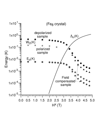
Figure 1: $Fe_{8}$ crystal (cluster of $50^{3}$ $Fe_{8}$ molecules, for details see Appendix B). The curves are: circles - half-width $W_{D}$ of the dipolar bias distribution vs transverse field $H^{x}$ (in Tesla) for model depolarized sample (see the text); stars - $W_{D}(H^{x})$ for polarized sample; triangles - same as circles, but for the field-compensated sample; diamonds - half-width $E_{o}$ of the hyperfine bias distribution; squares - same as diamonds but for the field-compensated sample; solid line - tunneling matrix element $\Delta_{o}(H^{x})$. All molecules are in a state $|\Uparrow\rangle$. ($W_{D},\;E_{o},\;\Delta_{o}$ are in Kelvins.)

When $\Delta_{o}<<W_{D}$, in a depolarized sample the value of $W_{D}$ is several times larger than in a polarized sample. To understand how $W_{D}$ behaves at large transverse fields, it is sufficient to calculate this parameter in a model depolarized sample where all molecules are in states $|\Uparrow\rangle$, but $\sum_{i}S^{z}_{i}/|S^{z}_{i}|=0$. SxSign The transverse field dependence of important parameters for crystals of $Fe_{8}$ and $Mn_{12}$ molecules is presented in Figs.1 and 2 (the description of our calculation procedure is given in Appendix B). RES_EX Deviations from the results of Figs.1 and 2 for nonzero populations of states $|\Downarrow\rangle$ are insignificant up to the limit of equipopulation - this is clear, for example, from Fig.5 (Appendix B).

Depending on the crystal structure and the sample geometry, the dipolar fields distribution can be shifted (such a shift can be rather large, see, for example, Fig.5 in Appendix B). This shift changes with the transverse field. The larger the shift, the slower both the $W_{D}(H^{\perp})$ and the $E_{o}(H^{\perp})$ decrease with $H^{\perp}$. This effect can be seen in the high-field part of Fig.1. Two upper curves for both $W_{D}$ and $E_{o}$ represent the results of calculations in our $Fe_{8}$ cluster ”as it is” (with no longitudinal field compensation). To obtain the two lower curves for both $W_{D}$ and $E_{o}$, the corresponding external longitudinal field was applied for each value of the external transverse field to shift a position of the longitudinal fields distribution back to zero (the longitudinal field compensated sample). The shift in our $Mn_{12}$ sample is small.

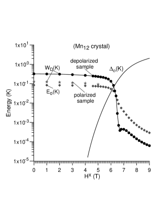
Figure 2: $Mn_{12}$ crystal (cluster of $50^{3}$ $Mn_{12}$ molecules; no ”faster relaxing species” DeltaDistr ; WWEPL ). The curves are: solid line with circles - $W_{D}(H^{x})$ for ”depolarized” sample; stars - $W_{D}(H^{x})$ for polarized sample; diamonds - $E_{o}(H^{x})$; solid line - $\Delta_{o}(H^{x})$.

(5) NPC-window.   When studying the spin dynamics in the NPC-window, one needs to know the region of the field where this window is situated. This window can be rather narrow and for our examples of the $Fe_{8}$ and the $Mn_{12}$ systems this can be seen in Fig.3. Since we are not going to discuss here a coherence optimization strategy, STPRB in this Figure we present the transverse field behavior of the dimensionless decoherence rates $\gamma^{nu}_{\phi}$ and $\gamma^{ph}_{\phi}$, Eq.(1), for external field along the $x$ axis only and for molecules containing only natural isotopes. NatIsot (Note that both rates are almost insensitive to changes in the populations of states $|\Uparrow\rangle$ and $|\Downarrow\rangle$.) The small oscillation energy $\Omega_{o}$ is $\sim E_{g}$ and, like $E_{g}(H^{\perp})$, slowly decreases with $H^{\perp}$. In zero field $\Omega_{o}=2SC_{\perp}(DE)^{1/2}$ ($C_{\perp}\approx 1.56$) for $Fe_{8}$ and $\Omega_{o}\sim 2SD$ for $Mn_{12}$. TB The Debye energy $\Theta_{D}$ for $Fe_{8}$ and $Mn_{12}$ is known experimentally. Debye_MnFe

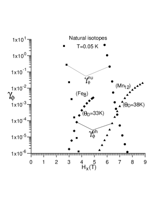
Figure 3: The transverse magnetic field behavior of the dimensionless decoherence rates $\gamma^{nu}_{\phi}$ (shown by squares and circles) and $\gamma^{ph}_{\phi}$ (diamonds and triangles) at azimuthal angle $\varphi=0$ (i.e., along the $x$-axis) for $Fe_{8}$ (squares and diamonds) and $Mn_{12}$ (circles and triangles) systems at $T=0.05\;K$. The results are presented for the natural isotopes ($Fe^{56},\;H^{1},\;Br^{79},\;N^{14},\;C^{12}$ and $O^{16}$ species for $Fe_{8}$ molecule and $Mn^{55},\;H^{1},\;C^{12}$ and $O^{16}$ species for $Mn_{12}$ molecule).

III Multimolecular processes in the limit $\Delta_{o}>>\{W_{D},E_{o},\hbar/\tau_{np}\}$

If in the NPC-window the half-width $W_{D}$ of the dipolar bias distribution is larger than $\Delta_{o}$, any spin dynamics is, in general, incoherent. Outside of this window, independently of the ratio $\Delta_{o}/W_{D}$, the spin dynamics is also incoherent. In this Section we study the multimolecular correlations induced by the dipole-dipole interactions between molecules in states $|\Uparrow\rangle$ and $|\Downarrow\rangle$ in the NPC-window. We assume that in the region of fields of our interest $\Delta_{o}>>\{W_{D},E_{o},\hbar/\tau_{np}\}$ (like, for example, in the region $3.5<H^{x}<4.2\;T$ for $Fe_{8}$ and in the region $6.7<H^{x}<7.4\;T$ for $Mn_{12}$, see Fig.3).

III.1 One-pair processes

At very low temperatures, when only two lowest states of each molecule are occupied, in the limit $\Delta_{o}>>\{W_{D},E_{o},\hbar/\tau_{np}\}$ we work in the representation (27) $\{|\Uparrow\rangle,|\Downarrow\rangle\}$ of the Hamiltonian (26) (Appendix A). Consider one pair of interacting molecules in the sample (Appendix C). Such a pair is described by the Hamiltonian (32) ($\xi_{i}$ is the bias energy; in general, it is the time-dependent parameter) and can be found in four states: $|\Uparrow_{1}\Uparrow_{2}\rangle;\;|\Uparrow_{1}\Downarrow_{2}\rangle;\;|\Downarrow_{1}\Uparrow_{2}\rangle;\;|\Downarrow_{1}\Downarrow_{2}\rangle$. In the limit $\Delta_{o}>>|V^{\alpha\beta}_{dd}|$ two central ”flip-flop” states $|\Uparrow_{1}\Downarrow_{2}\rangle$ and $|\Downarrow_{1}\Uparrow_{2}\rangle$, linked by the effective tunneling matrix element

$$\Delta_{ff}\sim|V^{zz}_{dd}(R)|{\Delta_{1}\Delta_{2}\over\varepsilon_{1}\varepsilon_{2}}$$ (9)

(only the largest term in $B(\vec{R})$ Eq.(35) is shown - its form is similar to that known from the theory of dielectric glasses Laikhtm ; BurKag ), can be considered as an effective two-level system with the asymmetry

$$\xi_{ff}\approx|\varepsilon_{1}-\varepsilon_{2}|\sim|\xi^{2}_{1}-\xi^{2}_{2}|/2\Delta_{o}<<\Delta_{o}$$ (10)

(recall that all $\Delta_{i}$ are supposed to be the same). Note that all $V^{\alpha\beta}_{dd}(R)$ are independent of the external field.

Two other states are separated from the two flip-flop states by the energy gaps $>\Delta_{o}$ and in the region of fields where $\Delta_{o}>|V^{\alpha\beta}_{dd}|$, their effect on the flip-flop transitions is small. If $\Delta_{ff}>\xi_{ff}$, two flip-flop states are in resonance and the amplitude of oscillations (with frequency $E_{ff}\sim(\xi^{2}_{ff}+\Delta^{2}_{ff})^{1/2}$, (37)) between them is $\approx 1$. At the same time, transitions between other states are not in resonance (they are accompanied by the energy change $>\Delta_{o}$) and their amplitude is $\lesssim(V^{\alpha\beta}_{dd})^{2}\xi^{2}_{i}/\Delta^{4}_{i}$.

In the field region where $\Delta_{o}\lesssim|V^{\alpha\beta}_{dd}|$ it is more convenient to solve the problem for the dynamics of a pair of interacting spins in the basis set (28). DubSt However, in this limit it can be rather difficult (or even impossible) to observe coherent dynamics in an ensemble of spins. First of all, in this limit $W_{D}$ also can be $\gtrsim\Delta_{o}$ (like in $Fe_{8}$ and $Mn_{12}$). Moreover, the variety of different collective processes leads to additional phase randomness and, consequently, to suppression of coherence.

In what follows we suppose to work only in the part of the NPC-window where $\Delta_{o}>|V^{\alpha\beta}_{dd}|$ and the probability to observe coherent spin dynamics is larger.

At low temperatures ($k_{B}T<\Delta_{o}$) a number of the molecules in the excited state $|\Downarrow\rangle$ with energy $+\varepsilon$ can be estimated as $N_{ex}(T)\sim N_{o}e^{-\varepsilon/k_{B}T}/(e^{-\varepsilon/k_{B}T}+e^{\varepsilon/k_{B}T})\sim N_{o}e^{-2\Delta_{o}/k_{B}T}$ ($N_{o}$ is the total number of molecules) and is small compared to the number of the ground state molecules. These excited molecules are uniformly distributed over the sample, and each of them is surrounded by the $\sim N_{o}/N_{ex}$ ground state molecules. The excited molecule can be in a ”flip-flop resonance” with the ground state molecule only if $\xi_{ff}\lesssim\Delta_{ff}$. The time needed for the flip-flop transition to happen is $\sim\hbar/\Delta_{ff}\sim O(R^{3})$ and the fastest transitions are expected to be between the nearest-neighbor molecules. For the effective two-level systems composed of the two nearest-neighbor molecules we introduce the corresponding effective tunneling matrix element $\Delta^{nn}_{ff}$ and the asymmetry $\xi^{nn}_{ff}$.

In a simple cubic lattice each excited molecule can make a flip-flop transition with any of its six nearest-neighbor ground state molecules with the same probabilities. In a generic lattice these probabilities can be different since $\Delta^{nn}_{ff}$ depends on the lattice structure. The average over three crystallographic axes value of the $\Delta^{nn}_{ff}$ is $\sim W_{D}(H^{\perp}=0)$ for polarized sample, see Figs.1 - 2 ($W_{D}(0)$ for polarized sample is $\sim E_{D}/V^{(1)}_{o}$, where $V^{(1)}_{o}$ is the volume per one molecule).

If $\Delta^{nn}_{ff}>\xi^{nn}_{ff}$ for the overwhelming majority of the nearest-neighbor molecules (this issue is discussed in Section IV.1), it is unlikely that at low temperatures any resonant pair of the nearest-neighbor molecules (say, $i$-th and $j$-th molecules) will remain in resonance for a long time. Instead, since the total probability for the excited molecule (either $i$-th, or $j$-th, as a result of oscillations (36)) to create a resonance with one of the other five nearest-neighbor molecules is larger than the probability to remain in resonance with the same molecule all the time $t\sim\tau_{np}$, the fastest flip-flop transitions can ”propagate” through the crystal involving more and more new molecules. Of course, not only the nearest-neighbor molecules can be involved, but also the ”lengthy” pairs (with $\Delta_{ff}(R)<\Delta^{nn}_{ff}$). However, flip-flop transitions between the nearest-neighbor molecules are faster.

In what follows, for brevity, these ”mobile” (or ”potentially mobile”) flip-flop transitions between the states $|\Uparrow\rangle$ and $|\Downarrow\rangle$ in the nearest-neighbor molecules will be called ”flipons” (a kind of magnon). The number of flipons is determined by the number of excited molecules $N_{ex}(T)$. In a generic lattice $\Delta^{nn}_{ff}$ can be different along different crystallographic axes. However, if flipon moves along one axis and for this axis $\{(\Delta^{nn}_{ff})_{i}\}$ are large in comparison with $\{(\xi^{nn}_{ff})_{i}\}$, such a movement is, in some sense, ”coherent” since flipon leaves site $i$ only because of equal probabilities for the excited spin to create a resonance with both of its nearest neighbors along this axis.

It is worth mentioning that, if there is a whole distribution of $\Delta_{o}$ (say, if there are ”faster relaxing species” DeltaDistr ; WWEPL ) in a sample, the fraction of resonant flip-flop molecules decreases. This is because in such a sample for some fraction of pairs the asymmetry $\xi_{ff}$ can be $\sim\Delta_{o}$ (and $\Delta_{o}$ increases with $H^{\perp}$). These impurities can essentially limit (or even completely block) the motion of flipons.

III.2 Multi-pair processes

On average, two nearest-neighbor excited molecules are separated by the distance

$$R_{ex}(T)\sim(V^{(1)}_{o}N_{o}/N_{ex})^{1/3}.$$ (11)

At $k_{B}T<<\Delta_{o}$, $R_{ex}(T)$ is large compared to $\widetilde{a}\equiv(V^{(1)}_{o})^{1/3}$ (in a cubic lattice $\widetilde{a}\equiv a$; $a$ is the lattice constant). Consider two pairs of the resonant nearest-neighbor molecules and let the distance between these pairs be $R$. This group of four molecules contains two excited molecules (with energies $\varepsilon_{2},\;\varepsilon^{{}^{\prime}}_{2}$) and two ground state molecules (with energies $\varepsilon_{1},\;\varepsilon^{{}^{\prime}}_{1}$). In the limit $\Delta_{o}>>\{W_{D},E_{o},\hbar/\tau_{np}\}$ and $\Delta_{o}>|V^{\alpha\beta}_{dd}|$ both these resonant pairs experience mainly the flip-flop transitions.

If $R>>\widetilde{a}$, the strength $|V^{\alpha\beta}_{dd}(R)|$ of the interactions between molecules belonging to different pairs is $<\Delta^{nn}_{ff}$. Then, using the same arguments as for one pair of molecules, in the case of two resonant pairs we can also consider only corresponding collective ”flip-flop” transitions between the eigenstates of each resonant pair. The effective tunneling matrix elements connecting these collective flip-flop states (separated from all other states by the energy gaps $>\Delta^{nn}_{ff}$) is

$$\Delta^{(2)}_{ff}(\vec{R})\sim|V^{zz}_{dd}(\vec{R})|{\Delta^{nn}_{ff}\Delta^{{}^{\prime}nn}_{ff}\over E^{nn}_{ff}E^{{}^{\prime}nn}_{ff}},$$ (12)

where $E^{nn}_{ff}\sim((\xi^{nn}_{ff})^{2}+(\Delta^{nn}_{ff})^{2})^{1/2}$. Similarly to the case of one pair of molecules, these collective flip-flop states can also be considered as an effective two-level system with the asymmetry

$$\xi^{(2)}_{ff}\sim|E^{nn}_{ff}-E^{{}^{\prime}nn}_{ff}|.$$ (13)

Note that we deliberately consider two pairs of nearest-neighbor molecules since transitions between such molecules are faster, and in the limit of our interest the probability to find them in resonance is larger.

The effective matrix element $\Delta^{(2)}_{ff}$ describes the flip-flop transitions between the eigenstates of two resonant pairs (i.e., of two effective TLS). If $\Delta^{(2)}_{ff}>\xi^{(2)}_{ff}$, two resonant pairs are in resonance with each other. The flip-flop transitions between the eigenstates $|\Uparrow\rangle$ and $|\Downarrow\rangle$ of each molecule inside of one resonant pair are described by the matrix element $\Delta^{nn}_{ff}$. Then, since $\Delta^{nn}_{ff}>\Delta^{(2)}_{ff}$, the frequency of oscillations between states $|\Uparrow\rangle$ and $|\Downarrow\rangle$ of each molecule in such a resonant group of four molecules is $\sim\Delta^{nn}_{ff}$, but the group correlation time is $\sim\hbar/\Delta^{(2)}_{ff}$.

In a generic lattice, if the nearest-neighbor molecules in two pairs are located along different axes, the asymmetry $\xi^{(2)}_{ff}$ can be $\sim\Delta^{nn}_{ff}>>\Delta^{(2)}_{ff}$ and such two pairs can be out of resonance. However, if molecules in both pairs are located along the same axis (with a lattice constant $a$) and if $\Delta^{nn}_{ff}>>\xi^{nn}_{ff}$, the asymmetry is

$$\xi^{(2)}_{ff}\sim|V^{zz}_{dd}(a)|f(\xi_{i}/\Delta_{o}),\;\;\;f(\xi_{i}/\Delta_{o})\sim O(\xi^{2}_{i}/\Delta^{2}_{o}),$$ (14)

where the average value of $f(\xi_{i}/\Delta_{o})$ can be estimated roughly as $\sim W^{2}_{D}/\Delta^{2}_{o}$. Then, for the average asymmetry one gets $\widetilde{\xi}^{(2)}_{ff}\sim|V^{zz}_{dd}(a)|(W_{D}/\Delta_{o})^{2}<<|V^{zz}_{dd}(a)|$ and for such pairs the condition $\Delta^{(2)}_{ff}\gtrsim\xi^{(2)}_{ff}$ can be, in principle, fulfilled (actually, the difference of two mean energies $A$ and $A^{{}^{\prime}}$ (35) also contributes to $\xi^{(2)}_{ff}$ and this gives a similar effect). The term neglected in (14) is $\sim(\Delta^{nn}_{ff}/W_{D}(H^{\perp}))^{2}$ times smaller than the retained one - in the field region of our interest in most systems $\Delta^{nn}_{ff}(\widetilde{a})/W_{D}(H^{\perp})>>1$.

Note that for resonant pairs composed of the flip-flop molecules with $\Delta_{ff}(R)<<\Delta^{nn}_{ff}$, the glass-like scenario BurKag can be realized. In this case two pairs can be in resonance only if $\Delta^{(2)}_{ff}\sim\Delta_{ff}$ (for most of such pairs $\xi^{(2)}_{ff}\sim\Delta_{ff}$).

Knowing the sample average value of the asymmetry $\widetilde{\xi}^{(2)}_{ff}$, from the requirement $\Delta^{(2)}_{ff}(\vec{R})>\xi^{(2)}_{ff}$ one can estimate the average ”resonant” distance between two pairs:

$$R^{(2)}_{res}(H^{\perp})\sim[V^{(1)}_{o}\widetilde{V}_{dd}/\widetilde{\xi}^{(2)}_{ff}(H^{\perp})]^{1/3},$$ (15)

where NN_Str $\widetilde{V}_{dd}\sim E_{D}/V^{(1)}_{o}$. If $R<R^{(2)}_{res}$, two pairs could be, in principle, in resonance with each other. However, even if $\widetilde{\xi}^{(2)}_{ff}\to 0$, not any two pairs are in resonance since if $R>R_{ph}$, where

$$R_{ph}(T,H^{\perp})\sim[V^{(1)}_{o}\widetilde{V}_{dd}\tau^{ph}_{\phi}(T,H^{\perp})/\hbar]^{1/3},$$ (16)

the two-pairs correlation time is longer than incoherent phonon-assisted transitions in each molecule. Only the pairs satisfying the condition $R<R_{m}=\min\{R^{(2)}_{res},R_{ph}\}$, can be in resonance. Thus, if $R_{ex}(T,H^{\perp})<R_{m}$, most of the closest pairs of resonant molecules are able to come into resonance with each other. This happens at temperatures $T>T_{M}$,

$$T_{M}=\max\{T^{(2)}_{res},T_{ph}\},$$ (17)

with $T^{(2)}_{res}$ and $T_{ph}$ given by ($k_{B}T<\Delta_{o}$):

$$k_{B}T^{(2)}_{res}(H^{\perp})\sim 2\Delta_{o}/\ln[\widetilde{V}_{dd}/\widetilde{\xi}^{(2)}_{ff}],$$ (18)

$$k_{B}T_{ph}(H^{\perp})\sim 2\Delta_{o}/\ln[\Theta^{4}_{D}\widetilde{V}_{dd}/S^{2}\Omega^{2}_{o}\Delta^{3}_{o}].$$ (19)

If at these conditions $\tau_{np}>t_{c}$, where

$$t_{c}\sim\hbar/|V^{zz}_{dd}(R_{ex})|\sim(\hbar/\widetilde{V}_{dd})(R^{3}_{ex}/V^{(1)}_{o}),$$ (20)

at $t\gtrsim t_{c}$ the whole hierarchy of (more or less) correlated flip-flop clusters of the increasing ”size” $n$ (the number of involved resonant flip-flop pairs) can, in principle, appear. The time $t_{c}$ estimates the cluster correlation time.

Note, however, that if $\Delta^{nn}_{ff}>\xi^{nn}_{ff}$ for most of the nearest-neighbor molecules, instead of interactions between fixed pairs of resonant molecules, in the limit of our interest we have a set of flipons moving through the sample and interacting with each-other. At $T<T_{M}$ they participate in the collective processes very rarely (interactions can be neglected). When temperature increases, the number of flipons also increases and collective processes become more frequent. At $T>T_{M}$ correlations between flipons, in principle, may still lead to the creation of correlated clusters. However, due to various decorrelation (dephasing) processes, these clusters can be destroyed rapidly (or they will not be able to appear at all). Such dephasing processes will be considered in Section III.3.

III.3 Decorrelation

(1) Flipon motion.   If flipons are delocalized, the effective tunneling matrix element $\Delta^{(2)}_{ff}$ changes with the distance between flipons resulting in the suppression of correlations in clusters (if they appear).

Suppose that at $t=0$ there is a correlated cluster ($T_{M}<T<\Delta_{o}/k_{B}$) composed of nearly equidistant flipons (with distance $\approx R_{ex}$). If $\Delta^{nn}_{ff}>>\xi^{nn}_{ff}$ and if the flipons move along the same axis, correlations between them will not necessarily be destroyed immediately after the first ”jump”. Of course, if at $t>0$ the flipons start to move along different axes, in a generic lattice any correlations can be destroyed almost immediately (i.e., at $t\gtrsim\hbar/\Delta^{nn}_{ff}$) since in this case $\xi^{(2)}_{ff}$ can become $\sim\Delta^{nn}_{ff}>>\Delta^{(2)}_{ff}$. Note, however, that the flipons have larger probability to move along the axis with shortest lattice constant. Then, if we consider only a quasi-$1d$ motion of flipons (i.e., along the same axis), we can estimate the longest ”motional” dephasing time $\tau^{m}_{d}$. Comparison of this time with the cluster correlation time $t_{c}$ ($t_{c}<\tau_{np}$) shows whether the correlated cluster with the average distances $R_{ex}$ between the nearest-neighbor flipons can appear.

For the sake of simplicity, we approximate the flipon centers of mass motion by the discrete ”random walks” model (Appendix D). At $t>0$ the distances $R(t)$ between the nearest-neighbor flipons in the whole cluster become distributed around $R_{ex}$ with nonzero half-width $\delta R(t)$. Thus, instead of a single ”line” $\Delta^{(2)}_{ff}(R_{ex})$ one also gets a whole distribution of values $\Delta^{(2)}_{ff}(R)$ with nonzero mean-square deviation $\delta\Delta^{(2)}(t)=\langle(\Delta^{(2)}_{ff})^{2}-\langle\Delta^{(2)}_{ff}\rangle^{2}\rangle^{1/2}$. Knowing $\delta\Delta^{(2)}(t)$, the motional dephasing time can be obtained from the condition

$$\tau^{m}_{d}=t_{f}N^{m}_{d};\;\;\sum^{N^{m}_{d}}_{N=0}t_{f}\delta\Delta^{(2)}(N)\sim\hbar;\;\;t_{f}=\hbar/\Delta^{nn}_{ff}$$ (21)

for $N=t/t_{f}$ (or from the condition $\int^{\tau^{m}_{d}}_{0}dt\;\delta\Delta^{(2)}(t)\sim\hbar$ at large values of $N$). Obviously, the correlations in the whole cluster will be destroyed together with the destruction of resonances between the nearest-neighbor flipons. Since in each pair both flipons can move, for $\langle\Delta^{(2)}_{ff}\rangle$ we have

$$\sim\sum^{N}_{\widetilde{r}_{1},\widetilde{r}_{2}=-N}|V^{zz}_{dd}(R_{ex}+(\widetilde{r}_{1}-\widetilde{r}_{2})\widetilde{a})|P_{N}(\widetilde{r}_{1})P_{N}(\widetilde{r}_{2})$$ (22)

with the condition $(R_{ex}+(\widetilde{r}_{1}-\widetilde{r}_{2})\widetilde{a})/R_{ex}\geq\eta(T)$. Here $\eta(T)$ is the dimensionless (in units of $R_{ex}(T)$) minimally possible distance between the centers of mass of two flipons. Each distribution $P_{N}(\widetilde{r}_{i})$ gives the probability to find the $i$-th flipon at the distance $\widetilde{r}_{i}\widetilde{a}$ ($\widetilde{r}_{i}<N$) from its $t=0$ position after total $N$ steps (Appendix D). 2FDF

The solution of Eq.(21) depends on $\eta$ and $\rho$ (Eq.(42)) and can be found numerically. For $p=q=s=1/3$ (Eq.(39)) and $\rho=2/3$ we get

$$\tau^{m}_{d}=N^{m}_{d}t_{f}\equiv 3\lambda(\eta)[R_{ex}/\widetilde{a}]^{2}t_{f}\sim 3\lambda(\eta)[\widetilde{a}/R_{ex}]t_{c}.$$ (23)

If $\eta=2\widetilde{a}/R_{ex}$, for $0.05\leq\eta\leq 2/3$ we get $\lambda\equiv\lambda_{2}\approx 1.6\eta^{2}+0.35\eta+0.045$. If $\eta=\widetilde{a}/R_{ex}$, for $0.05\leq\eta<1/2$ we get $\lambda\equiv\lambda_{1}\approx 0.34\eta^{2}+0.2\eta+0.03$. Note that the configurations of the nearly equidistant flipons with $R_{ex}=\widetilde{a}$ do not exist, in contrast to those with $R_{ex}=2\widetilde{a}$. However, if flipons move along the same axis, but in the nearest-neighbor rows, the centers of mass of some flipons can be separated by the distance $\widetilde{a}$. To take this effect into account, one can use $\lambda=(\lambda_{2}+\lambda_{1})/2$ for estimations.

The answer for $\tau^{m}_{d}$ can be found in the equivalent dimensionless form $D_{f}\tau^{m}_{d}/R^{2}_{ex}=\widetilde{\lambda}(\eta,\rho)$, where $D_{f}$ is the flipon effective diffusion coefficient (42) and at $\rho=2/3$, $\widetilde{\lambda}(\eta,\rho)\equiv\lambda(\eta)$ from Eq.(23). The $\rho$-dependence of $\tau^{m}_{d}$ is roughly $\sim\rho^{-1/3}$. Then, $\tau^{m}_{d}/t_{c}$ can become larger either (i) at $T\to\Delta_{o}/k_{B}$, when flipons are in their dense phase and essentially localized ($\delta R(t)\to 0$); or (ii) if $s=1-p-q\to 1$, $\rho\to 0$ and flipons are almost immobile even at $T<\Delta_{o}/k_{B}$. The latter can be, in principle, realized in a sample with impurities.

If $\tau^{m}_{d}(T)<<t_{c}(T)$, the creation of a correlated cluster at the average distance $R_{ex}(T)$ is virtually impossible. Solving either the equation $N^{m}_{d}(R_{c})t_{f}=t_{c}(R_{c})$, or the equation

$$D_{f}t_{c}(R_{c})/R^{2}_{c}=\widetilde{\lambda}(\eta_{c},\rho),$$ (24)

one finds the average distance $R_{c}$ and the temperature

$$k_{B}T_{c}\sim 2\Delta_{o}(H^{\perp})/\ln[(R_{c}/\widetilde{a})^{3}-1]$$ (25)

at which $\tau^{m}_{d}\sim t_{c}$ and cluster can appear. For $\rho=2/3$ and $\eta_{c}=2\widetilde{a}/R_{c}$ we get $R_{c}\sim 3\widetilde{a}$ and $k_{B}T_{c}\sim 0.6\Delta_{o}(H^{\perp})$. For $\rho=2/3$ and $\eta_{c}=\widetilde{a}/R_{c}$ we get $R_{c}\sim 2\widetilde{a}$ and $T_{c}\sim\Delta_{o}(H^{\perp})$. These estimations shows that, if the scenario with $p\approx q\approx s\approx 1/3$ is realized, $\tau^{m}_{d}(T)<t_{c}(T)$ almost everywhere except the flipons dense phase at $T\to\Delta_{o}/k_{B}$, where $\tau^{m}_{d}(T)\sim t_{c}(T)$ and where $t_{c}(T)$ decreases itself (as well as $\tau_{np}(T)$, see Eq.1). If, in contrast, $s\to 1$ and $\rho\to 0$, $\tau^{m}_{d}>>t_{c}$ and correlated clusters can appear even at $T_{M}<T<T_{c}$.

(2) ”Spectral diffusion”.   The above described picture is valid only if $\Delta^{nn}_{ff}>\xi^{nn}_{ff}$ for most of the nearest-neighbor molecules. In the opposite limit, at $T>T_{M}$ the correlated clusters will be composed of almost immobile ”lengthy” flip-flop pairs with $\Delta_{ff}(R>\widetilde{a})<\Delta^{nn}_{ff}$, satisfying the condition $\Delta_{ff}\sim\Delta^{(2)}_{ff}$. This scenario is very similar to that in dielectric glasses BurKag and the cluster dephasing time at $t<\tau_{np}$ will be determined by the process similar to the ”spectral diffusion” in glasses. Laikhtm ; KlBlPh The change of states of fixed effective TLS results in the bias fluctuations and, consequently, in the dephasing. In this limit ($\Delta^{nn}_{ff}<\xi^{nn}_{ff}$) the cluster ”spectral diffusion” dephasing time $\tau^{s}_{d}$ is $\sim t_{c}$ since the asymmetry $\xi^{(2)}_{ff}$ for most groups of two resonant pairs is $\sim\Delta_{ff}$.

In the limit $\Delta^{nn}_{ff}>\xi^{nn}_{ff}$ the spectral diffusion-like process can contribute as well. Instead of going deeply into the details, here we only estimate the corresponding effects. Consider, for simplicity, the case of immobile flipons. The bias $(\xi^{nn}_{ff})_{i}$, acting on any $i$-th flipon, contains contributions from all individual spins in the sample. When any $j$-th flipon makes a transition, the change of the bias, acting on $i$-th flipon, is $\delta^{f}_{ij}(R_{ij})\sim V^{zz}_{dd}(R_{ij})\;(\xi^{nn}_{ff})_{i}(\xi^{nn}_{ff})_{j}/(E^{nn}_{ff})_{i}(E^{nn}_{ff})_{j}$. (Here $(\xi^{nn}_{ff})_{i,j}$ can be both positive and negative and the term $V^{zx}_{dd}\tau^{z}_{i}\tau^{x}_{j}$ does not change its sign when $j$-th flipon makes transition.) Then, if $N_{t}$ flipons make a transition ($\max(N_{t})=N_{ex}$), the total change of the bias acting on $i$-th flipons is $\delta^{f}_{i}=\sum^{N_{t}}_{j=1}\delta^{f}_{ij}(R_{ij})$.

Depending on the degree of ”polarization” $M_{t}=(N_{gs}-N_{es})/(N_{gs}+N_{es})$ of the group of $N_{t}$ flipons ($N_{gs}$ and $N_{es}$ are the numbers of flipons in their ground and excited states), the total bias change $|\delta^{f}_{i}|$ can vary roughly from $\widetilde{\delta}^{f}_{i}\sim|V^{zz}_{dd}(R_{ex})|\;[(\xi^{nn}_{ff})_{i}/(\Delta^{nn}_{ff})_{i}][\widetilde{\xi}^{nn}_{ff}/\widetilde{\Delta}^{nn}_{ff}]$ to $\sim\widetilde{\delta}^{f}_{i}\ln(N_{t})$ ($\widetilde{\Delta}^{nn}_{ff}$ is the sample average value of $(\Delta^{nn}_{ff})_{j}$ and $\widetilde{\xi}^{nn}_{ff}$ is the sample average absolute value of $(\xi^{nn}_{ff})_{j}$). Then the shortest dephasing time $\tau^{s}_{d}$ is $\sim t_{f}$. However, the dipole-dipole interaction changes its sign with the direction of $\vec{R}_{ij}$ and, on average, in the case $M_{t}\to 1$ the ”surface” spins will mainly determine the maximum value of the bias change $|\delta^{f}_{i}|$. For spins (flipons) in the bulk this essentially reduces $|\delta^{f}_{i}|$ and increases $\tau^{s}_{d}$.

If $M_{t}\to 0$, simultaneous transitions of many flipons nearly cancel the effect of each other resulting in $|\delta^{f}_{i}|\lesssim\widetilde{\delta}^{f}_{i}<<|V^{zz}_{dd}(R_{ex})|<<\Delta^{nn}_{ff}$. In this case the spectral diffusion mechanism cannot destroy the resonance neither inside of the individual flipons, nor between them. Indeed, the contribution from the $\xi^{nn}_{ff}$ to the asymmetry $\xi^{(2)}_{ff}$ in the limit $\Delta^{nn}_{ff}>\xi^{nn}_{ff}$ is $\sim(\xi^{nn}_{ff})^{2}/2\Delta^{nn}_{ff}$ and its change due to $\delta^{f}_{i}$ is $\sim\delta^{f}_{i}\;(\xi^{nn}_{ff})^{i}/(\Delta^{nn}_{ff})^{i}$.

On average, in a temperature equilibrated sample, it is plausible to assume $M_{t}\to 0$ and in the limit $\Delta^{nn}_{ff}>\xi^{nn}_{ff}$ the spectral diffusion effect is much weaker than the motional dephasing effect (broadening of the $\Delta^{(2)}_{ff}$ distribution due to the flipons motion). This remains valid also if the flipons are allowed to move. In this case the spectral diffusion dephasing time $\tau^{s}_{d}$ is roughly $\sim(\widetilde{\Delta}^{nn}_{ff}/\widetilde{\xi}^{nn}_{ff})^{3}$ times longer than the motional dephasing time $\tau^{m}_{d}$ (as it was already noted, if flipons move along different axis, in a generic lattice correlations can be destroyed already at $t\sim t_{f}$).

IV Discussion

In this Section we discuss a temperature equilibrated sample at $k_{B}T\lesssim\Delta_{o}$, where only the fraction $N_{ex}(T)$ of molecules are in the excited states $|\Downarrow\rangle$. Thus, we are not going to discuss the problem of the magnetization relaxation in the limit $\Delta_{o}>>\{W_{D},E_{o}\}$. If, for example, the sample is prepared at very high temperatures and then rapidly cooled down to low temperatures, it will start to relax to its temperature equilibrated state - this relaxation process will not be discussed here either.

If, in some system, in all the NPC-window $\Delta_{o}\lesssim|V^{\alpha\beta}_{dd}|$, it can be very difficult (most probably, impossible) to observe any coherent spin dynamics in an ensemble of interacting spins (Section III.1). Here we consider only the part of the NPC-window, where $\Delta_{o}>|V^{\alpha\beta}_{dd}|$. In both the $Fe_{8}$ and the $Mn_{12}$ systems, which are used in this work to illustrate how the problem can be analyzed, this field region is situated to the right of the minimum of $\gamma^{nu}_{\phi}+\gamma^{ph}_{\phi}$ (see Fig.3). The collective processes, having the largest amplitude in this region of fields, are the flip-flop processes.

IV.1 The ratio $\widetilde{\Delta}^{nn}_{ff}/\widetilde{\xi}^{nn}_{ff}$

The fastest pair flip-flop processes are the processes between the nearest-neighbor molecules. The average strength of the nearest-neighbor dipole-dipole interactions and the average value of the flipon effective tunneling matrix element $\widetilde{\Delta}^{nn}_{ff}$ are $\sim\widetilde{V}_{dd}$ ($\widetilde{V}_{dd}\sim 0.12\;K$ for $Fe_{8}$ and $\sim 0.07\;K$ for $Mn_{12}$). To find the average asymmetry $\widetilde{\xi}^{nn}_{ff}$, we first calculate the distributions $P_{12}(\varepsilon,H^{\perp})$ of the $\varepsilon=\varepsilon_{1}-\varepsilon_{2}$ ($\varepsilon_{i}=(\Delta^{2}_{i}+\xi^{2}_{i})^{1/2}$; all $\Delta_{i}$ depend on both the external and the dipolar transverse fields and are obtained by the exact diagonalization of (5) and (6), Appendix B), where $\varepsilon_{1,2}$ are for the nearest-neighbor molecules only. Then, we get $\widetilde{\xi}^{nn}_{ff}=(1/2)\int^{+\varepsilon_{o}}_{-\varepsilon_{o}}d\varepsilon\;|\varepsilon|P_{12}(\varepsilon,H^{\perp})$ ($\varepsilon_{o}$ is the maximum value of $\varepsilon$).

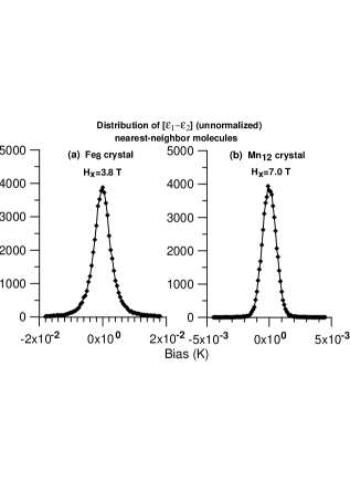
Figure 4: The distributions of the $\varepsilon=\varepsilon_{1}-\varepsilon_{2}$ for the nearest-neighbor molecules: (a) at $H^{x}=3.8\;T$ in the crystal of $Fe_{8}$ molecules (no field compensation); (b) at $H^{x}=7.0\;T$ in the crystal of $Mn_{12}$ molecules (no faster relaxing species). All cluster parameters are the same as in Figs.1 - 3. Here $\varepsilon$ is in Kelvins. The states $|\Uparrow\rangle$ and $|\Downarrow\rangle$ are equipopulated. Both distributions are averaged over three crystallographic axes.

For example, two distributions (at $H^{x}=3.8\;T$ for $Fe_{8}$ and at $H^{x}=7.0\;T$ for $Mn_{12}$) are presented in Fig.4. For these distributions we get $\widetilde{\xi}^{nn}_{ff}\approx 1.5\times 10^{-3}\;K$ for $Fe_{8}$ (with no field compensation) and $\widetilde{\xi}^{nn}_{ff}\approx 2.3\times 10^{-4}\;K$ for $Mn_{12}$ (the corresponding mean-square deviations $\delta\varepsilon=\langle\varepsilon^{2}-\langle\varepsilon\rangle^{2}\rangle^{1/2}$ are $\approx 4.7\times 10^{-3}\;K$ and $\approx 6.4\times 10^{-4}\;K$ respectively). For the field-compensated $Fe_{8}$ sample, the corresponding values are about two times smaller.

To summarize the results, we note that under the assumption of the absence of impurities with larger (or smaller) values of $\Delta_{i}$, in both systems in the NPC-window the average asymmetry $\widetilde{\xi}^{nn}_{ff}$ (as well as $\delta\varepsilon$) is small in comparison with $\widetilde{\Delta}^{nn}_{ff}$ for most of the nearest-neighbor molecules. In this case flipons can move in both systems.

Note, however, that in the $Mn_{12}$ crystal there are faster relaxing (minor) species DeltaDistr ; WWEPL (about $5-10\;\%$ of all molecules have lower potential barrier and larger values of $\Delta_{i}$) - these species can change somehow both the $\widetilde{\xi}^{nn}_{ff}$ and the $\delta\varepsilon$. In the NPC-window for major species the spin dynamics of these minor species is incoherent already. Since even the Hamiltonian for these minor species is still unknown (or unpublished), we cannot describe their effect quantitatively. Obviously, they can decrease the number of flipons and limit their motion.

IV.2 Collective spin dynamics

From Eqs.(18)-(19) in the $Fe_{8}$ crystal at $H^{x}=3.8\;T$ ($\Delta_{o}\approx 0.35\;K$) one finds $T_{M}\sim 0.1\;K$ for the field compensated sample ($T_{M}\sim 0.11\;K$ with no field compensation). The corresponding temperature for the $Mn_{12}$ crystal at $H^{x}=7.0\;T$ ($\Delta_{o}\approx 0.36\;K$) is $T_{M}\sim 0.13\;K$. At $T<T_{M}$ the average distance between flipons is large, and so the collective multi-pair flip-flop processes are essentially ”frozen” and correlated clusters of flipons can not appear.

At $T_{M}<T\lesssim\Delta_{o}/k_{B}$ the collective multi-pairs processes are unfrozen and, when the temperature increases, the whole hierarchy of correlated clusters of increasing size $n$ (the number of involved flipons, $\max\{n\}=N_{ex}(T)$) can, in principle, appear. The motion of flipons leads to the suppression of correlations. The spectral diffusion effect in the limit $\Delta_{o}>>\{W_{D},E_{o}\}$ is rather weak (Section III.3) and the spectral diffusion dephasing time $\tau^{s}_{d}$ is longer than the motional dephasing time $\tau^{m}_{d}$. If at certain temperature the cluster dephasing time $\tau^{ms}_{d}(T)=\min\{\tau^{m}_{d}(T),\tau^{s}_{d}(T)\}$ is shorter than the cluster correlation time $t_{c}(T)$, creation of the correlated clusters at average distance $R_{ex}(T)$ is virtually impossible. Instead, only short-living (with $\tau^{ms}_{d}<t_{c}<\tau_{nd}$) correlations between molecules at distances $R<R_{ex}$ can be present.

If flipons can move, the correlated clusters at average distance $R_{ex}$ can appear only at temperatures $T\gtrsim T_{c}>T_{M}$ (Eqs.(17, 25)), when $\tau^{m}_{d}$ becomes longer than $t_{c}$ and $R_{ex}(T)$ becomes shorter then $R_{c}$ (Eq.(24)). In $Fe_{8}$ (for $H^{x}=3.8\;T$) and in $Mn_{12}$ (for $H^{x}=7.0\;T$) crystals this may happen already at $T\sim 0.25\;K$ (assuming $p=q=s=1/3$ and $\rho=2/3$, see Section III.3). Note, however, that in the $Fe_{8}$ crystal for example, where all lattice constants are different, only flipons oriented (propagating) along the same crystallographic axis can create correlated cluster. At the same time, flipons have larger probability to propagate along the axis with the shortest inter-molecular distance (i.e., with larger $\Delta^{nn}_{ff}$). In this case a quasi-$1d$ motion of flipons is more probable than a $3d$ one. Nevertheless, if at $t>0$ flipons will start to change their orientation, this process will speed up decorrelation.

If the cluster dephasing time $\tau^{ms}_{d}$ is $\sim t_{c}<<\tau_{np}$ (Eq.2), during the time interval $t=\tau_{np}$ the correlated clusters can be created and destroyed (roughly) $\sim\tau_{np}/t_{c}$ times. During the cluster life-time $\tau^{ms}_{d}$ all molecules, belonging to cluster, can make $\sim\Delta^{nn}_{ff}t_{c}/\hbar$ coherent oscillations (36). At $T\sim 0.25\;K$ the correlated clusters can ”reappear” $\sim 50$ times in $Fe_{8}$ at $H^{x}=3.8\;T$ (for a cluster of flipons oriented along the same axis) and $\sim 10$ times in $Mn_{12}$ at $H^{x}=7.0\;T$. At these fields one may expect $\sim 30$ oscillations (36) in both $Fe_{8}$ and $Mn_{12}$. All these estimations do not take into account the coherence optimization strategy STPRB and we again assume $p=q=s=1/3$ and $\rho=2/3$. Note also that the phonon decoherence rate $\gamma^{ph}_{\phi}$ increases with temperature (see Eq.1), but at $k_{B}T<\Delta_{o}$ this increase is slow.

In the case of $Mn_{12}$, in the NPC-window for major species the spin dynamics of molecules belonging to minor species is incoherent already. Due to the difference in $\Delta_{i}$, the molecules of major and minor species cannot create correlated flip-flop pairs between each other. This results (i) in a decrease in the number of flipons; (ii) in partial localization of flipons (depending on the fraction of impurities); and (iii) in randomization of processes due to interactions between molecules belonging to different species. The last effect gives rise to the incoherent pair processes, leading to suppression of coherence.

The larger the concentration of impurities with incoherent internal dynamics, the smaller the probability for correlated clusters to appear. However, at $T>T_{c}$ the sample can become covered by correlated clusters of the sizes smaller than the average distance between impurities $R_{im}$. For example, in $Mn_{12}$ at $H^{x}=7.0\;T$ and $T=0.25\;K$ one gets $R_{ex}\sim 3\widetilde{a}$. If $R_{im}\gtrsim 10\widetilde{a}$, at these values of field and temperature the correlated clusters of the radius $\sim 3R_{ex}$ can, in principle, appear.

If $\Delta^{nn}_{ff}<\xi^{nn}_{ff}$ for most of the nearest-neighbor molecules (i.e., no flipons), the correlated clusters composed of lengthy flip-flop pairs with $\Delta_{ff}(R\sim R_{ex})<<\Delta^{nn}_{ff}$ can appear already at $T_{M}<T<T_{c}$. The asymmetry $\xi^{(2)}_{ff}$ for two resonant pairs in such a cluster is $\sim\Delta_{ff}\sim\Delta^{(2)}_{ff}$ and the cluster life-time is $\sim t_{c}$. This means that all resonant pairs will be able to make only one corelated flip-flop transition before correlations will be suppressed (if $t_{c}<<\tau_{np}$, such a cluster can reappear $\sim\tau_{np}/t_{c}$ times). If $\Delta^{nn}_{ff}>\xi^{nn}_{ff}$, but for some reason $\rho\to 0$ ($s\to 1$), the correlated clusters of immobile flipons can appear. Because of the weakening of the spectral diffusion effect in the limit $\Delta_{o}>>\{W_{D},E_{o}\}$, the dephasing time for these clusters can be limited only by $\tau_{np}$ and the number of oscillations (36) can be limited only by $Q_{\phi}\Delta^{nn}_{ff}/\Delta_{o}$.

V Summary

In the present work the internal dynamics of a temperature-equilibrated crystalline sample of the dipole-dipole interacting molecules with the central spins $\vec{S}_{i}$ has been studied in the coherence window for nuclear spin and phonon degrees of freedom.

At large external transverse magnetic fields the tunneling matrix element $\Delta_{o}$ (Section I and Appendix A) increases, whereas both the half-width of the dipolar bias distribution $W_{D}$ and the half-width of the hyperfine bias distribution $E_{o}$ decrease (Section II and Appendix B).

At a certain value of the transverse field, the coherence window for phonon and nuclear spin-mediated decoherence (the NPC-window) opens up (Sections I and II). Outside of the NPC-window the spin dynamics is incoherent. If in the whole NPC-window the average strength of the dipole-dipole interactions between the nearest-neighbor molecules $\widetilde{V}_{dd}$ or $W_{D}$ are larger than $\Delta_{o}$, the spin dynamics is also incoherent. In the opposite limit the coherent spin dynamics is possible.

In the limit $\Delta_{o}>\widetilde{V}_{dd}$ and if the effective matrix element $\Delta^{nn}_{ff}$, describing transitions between two flip-flop states of the nearest-neighbor molecules, Eq.(9), is large compared to the asymmetry $\xi^{nn}_{ff}$ of these two states, Eq.(10), the spin correlations between the nearest-neighbor molecules lead to the creation of resonant flip-flop pairs (Section III.1 and Appendix C). Such resonant pair experiences oscillations (36) between states $|\Uparrow\Downarrow\rangle$ and $|\Downarrow\Uparrow\rangle$ of two molecules with frequency $\sim\Delta^{nn}_{ff}$.

If $\Delta^{nn}_{ff}>\xi^{nn}_{ff}$ for the most pairs of the nearest-neighbor molecules, the resonant flip-flop transitions can ”propagate” in the crystal, involving more and more new molecules (one molecule in a pair remains in its ground state but another nearest-neighbor molecule creates new resonance with the excited molecule). This ”mobile” magnon-like process (a spin-excitation) between the states of two involved nearest-neighbor molecules in our work is called ”flipon” (Section III.1). The number of flipons is limited by the number of excited molecules $N_{ex}(T)$.

At $T<T_{M}=\max\{T^{(2)}_{res},T_{ph}\}$, Eqs.(18,19), the distances between flipons are long and the correlations between them are unimportant. At $T>T_{M}$ the correlations between flipons become crucial and at certain conditions can lead to the creation of correlated clusters of flipons (Section III.2). Each cluster represents a correlated group of molecules experiencing coherent oscillations (36) between their lowest states $|\Uparrow\rangle$ and $|\Downarrow\rangle$.

The flipons motion and the spectral diffusion process result in the suppression of correlations (Section III.3). If $\Delta^{nn}_{ff}>>\xi^{nn}_{ff}$ for most pairs of the nearest-neighbor molecules (Section IV.1) and flipons can move, the correlated cluster can appear only at $T\gtrsim T_{c}$, Eq.(25). The average inter-flipon distance in this case is given by the solution of Eq.(24) and the cluster dephasing time (i.e., its life-time) $\tau^{ms}_{d}$ is $\sim t_{c}$ (Eq.(20)). Molecules that belong to the cluster can make $\sim\Delta^{nn}_{ff}t_{c}/\hbar$ oscillations (36) before the correlations will be suppressed. During the total phonon/nuclear spin coherence time $\tau_{np}$, Eq.(2), the coherent clusters can ”reappear” $\lesssim\tau_{np}/t_{c}$ times. At $T<T_{c}$ only random short-living ($t<t_{c}$) correlations within small groups of flipons, separated by distances $R<R_{ex}(T)$, Eq.(11), can appear.

The smaller the effective flipon diffusion coefficient $D_{f}$, Eq.(42), the longer the cluster life-time $\tau^{ms}_{d}$. If, for some reason, the flipons are localized ($D_{f}\to 0$), the correlated clusters of immobile flipons can appear even at $T<T_{c}$. Their life-time can be limited only by $\tau_{np}$, and the number of oscillations (36) can be limited only by $Q_{\phi}\Delta^{nn}_{ff}/\Delta_{o}$. If $\Delta^{nn}_{ff}<\xi^{nn}_{ff}$, the correlated clusters of ”lengthy” resonant flip-flop pairs (molecules in these pairs are separated by the distance $R\sim R_{ex}$) can appear also at $T<T_{c}$. Their life-time is limited by $t_{c}$. On average, all pairs in these clusters will be able to make only one flip-flop transition before correlations will be suppressed. If $t_{c}<\tau_{np}$, these clusters can reappear several times.

It is worth mentioning also that various systems allow the coherence optimization strategy (orientation of external transverse field in a plane, chemical replacement of isotopes, etc. STPRB ) to be applied to get longer spin/phonon coherence time-interval $\tau_{np}$ or to shift the coherence window down to lower values of the transverse field.

This concludes our study of the collective spin dynamics of a temperature equilibrated sample in the coherence window for phonon and nuclear spin-mediated decoherence. The presented analysis can be applied to any crystalline nanomagnetic insulator composed of the central spin $\vec{S}$ molecules, and can be useful in the search for magnetic systems showing the spin coherence and collective phenomena. The analysis for the induced dynamics (when system at $t=0$ is prepared in some initial state) will be presented separately.

It is a pleasure to thank A. Morello for numerous helpful and motivating discussions. The author is grateful to R. Sessoli and W. Wersdorfer for providing him with complete files on the structure of the $Mn_{12}$-acetate molecule. The author is also indebted to S. Burmistrov, L. Dubovskii and I. Polishchuk for useful discussions. This work is supported by Russian grant RFBR 04-02-17363a.

Appendix A Two-level system

The effective Hamiltonin of a biased two-level system (TLS) has the form:

$$H_{TLS}=-\Delta_{o}\hat{\tau}^{x}-\xi\hat{\tau}^{z},$$ (26)

where $\hat{\tau}^{x},\hat{\tau}^{z}$ are the Pauli matrixes multiplied by 2; $\Delta_{o}$ is the tunneling matrix element; and $\xi$ is the asymmetry between two states (i.e., the longitudinal bias). One can easily solve this problem for eigenfunctions:

$$|\Uparrow\rangle = u|\uparrow\rangle+v|\downarrow\rangle;\;|\Downarrow\rangle=-v|\uparrow\rangle+u|\downarrow\rangle;\;$$

$$(u,v) = ((\varepsilon\pm\xi)/2\varepsilon)^{1/2};\;\;\;\varepsilon=\sqrt{\xi^{2}+\Delta^{2}_{o}},$$ (27)

where the corresponding energies in states $|\Uparrow\rangle,|\Downarrow\rangle$ are given by $E_{\Uparrow,\Downarrow}=\mp\varepsilon$ and

$$|\uparrow\rangle={{1}\choose{0}};\;\;\;|\downarrow\rangle={{0}\choose{1}}.$$ (28)

If at time $t=0$ system was in state $|\uparrow\rangle$, the probabilities to find system at time t in states $|\uparrow\rangle$ or $|\downarrow\rangle$ are

$$P_{\uparrow\uparrow}=1-{\Delta^{2}_{o}\over\varepsilon^{2}}\sin^{2}(\varepsilon t/\hbar);\;\;\;P_{\downarrow\uparrow}={\Delta^{2}_{o}\over\varepsilon^{2}}\sin^{2}(\varepsilon t/\hbar).$$ (29)

This describes the oscillations with frequency $\varepsilon$ between states $|\uparrow\rangle$ and $|\downarrow\rangle$. In the limit $\Delta_{o}<<\xi$ the oscillations are suppressed since their amplitude is $\Delta^{2}_{o}/\xi^{2}<<1$.

Appendix B Method of calculations

(1) $W_{D}(H^{\perp})$.   To obtain the transverse field behavior of the dipolar bias distribution half-width $W_{D}$ in the crystals of $Fe_{8}$ and $Mn_{12}$ molecules, two clusters of different crystal symmetry are used. (a) The $Fe_{8}$ crystal. The cluster for the $Fe_{8}$ system contains $50^{3}$ unit cells arranged in a triclinic lattice array with lattice parameters: CDC $a=10.522(7)$ Å; $b=14.05(1)$ Å; $c=15.(1)$ Å with angles $\alpha=89.90(6)^{o};\beta=109.65(5)^{o};\gamma=109.27(6)^{o}$. Each unit cell of volume $V_{o}\approx 1969$ ų contains eight spin-$5/2$ $Fe^{+3}$ ions, correctly positioned and oriented. CDC ; OrientFe (b) The $Mn_{12}$ crystal. The cluster for the $Mn_{12}$ system contains $50^{3}$ unit cells, arranged in a tetragonal lattice array with lattice parameters: CDC $a=b=17.1627(6)$ Å; $c=12.2880(4)$ Å with angles $\alpha=\beta=\gamma\approx 90^{o}$. Each unit cell of volume $V_{o}\approx 3619.5$ ų contains twelve spins: four spin-$3/2$ $Mn^{4+}$ ions in the inner shell and eight spin-$2$ $Mn^{3+}$ ions in the outer shell, correctly positioned and oriented. CDC

The distributions of the dipolar bias fields and energies in the cluster are calculated taking into account all internal spins $\vec{s}^{(p)}_{i}$ of each molecule ($\vec{S_{i}}=\sum_{p}\vec{s}^{(p)}_{i}$, $p=8$ in $Fe_{8}$ and $p=12$ in $Mn_{12}$). The internal molecular spins $\vec{s}^{(p)}_{i}$ cannot flip independently - each molecule changes its total spin orientation as a rigid object. Initially, all molecules in the sample are oriented along the easy axis, either at random with projections $S^{z}_{i}=\pm S_{i}$ (for depolarized sample with initial magnetization $M=0$), or with projections $S^{z}_{i}=+S_{i}$ (for polarized sample with $M=1$).

To obtain the average longitudinal bias field acting on $i$-th molecule, we calculate the longitudinal fields $h^{z(p)}_{i}$, created by all internal spins of all molecules in the sample at each $p$-th internal spin $\vec{s}^{(p)}_{i}$ of $i$-th molecule. Then, the average longitudinal field at $i$-th molecule is $H^{z}_{i}=\sum_{p}(s^{(p)}_{i}/S_{i})h^{z(p)}_{i}$. The calculation of the average transverse field is similar.

First, we calculate the longitudinal and transverse fields in the sample, assuming $S^{z}_{i}=S_{i}$ and $S^{x}_{i}=0$ for each molecule. Knowing internal and external longitudinal and transverse fields at each molecule from the first step, we calculate $\Delta_{i}$, $S^{z}_{i}$ and $S^{x}_{i}$ by means of exact diagonalization of the molecular Hamiltonians (5,6). Obtaining $S^{z}_{i}$ and $S^{x}_{i}$ for each molecule, we repeat calculation of fields in the sample. Using these new fields, we recalculate $\Delta_{i}$, $S^{z}_{i}$ and $S^{x}_{i}$ and so on. This iteration procedure converges and, depending on the value of external applied field, it is enough to make $10-20$ iterations to obtain a final result.

Figure 5: Total distributions of the internal dipolar fields in the crystal of $Fe_{8}$ molecules (cluster of $50^{3}$ molecules arranged in a triclinic lattice). The curves are: solid line - the transverse dipolar fields distribution for $M=1$ (polarized sample) at $H^{x}_{ext}=0$; inverse triangles - the longitudinal dipolar fields distribution for $M=1$ at $H^{x}_{ext}=4.8\;T$; squares - the longitudinal dipolar fields distribution for $M=0$ at $H^{x}_{ext}=4.8\;T$ (depolarized sample - states $|\Uparrow\rangle$ and $|\Downarrow\rangle$ are equipopulated); diamonds - the same as squares, but for the model depolarized sample (all molecules are in states $|\Uparrow\rangle$, but $\sum_{i}S^{z}_{i}/|S^{z}_{i}|=0$); circles - the longitudinal dipolar fields distribution for $M=1$ at $H^{x}_{ext}=0$ (polarized sample); triangles - the longitudinal dipolar fields distribution for $M=0$ at $H^{x}_{ext}=0$ (depolarized sample).

To show that this iteration procedure converges, we present Fig.5 where the total distributions of longitudinal and transverse fields in the crystal of $Fe_{8}$ molecules are plotted. In a completely polarized sample ($M=1$) at zero external transverse field $H^{x}_{ext}$ the ”$x$” component of the dipolar field is $H^{x}_{d}\sim Sz_{ij}x_{ij}/r^{5}_{ij}$ ($S^{x}=0$ and $S^{z}=S$). At large $H^{x}_{ext}$ ($S^{z}\to 0$ and $S^{x}\to S$) the ”$z$” component of the dipolar field is $H^{z}_{d}\sim Sx_{ij}z_{ij}/r^{5}_{ij}$. Thus, the $z$-fields distribution at large $H^{x}_{ext}$ and the $x$-fields distribution in a polarized sample ($M=1$) at $H^{x}_{ext}=0$ should be the same. This is what one can see in Fig.5. After the iteration procedure the longitudinal fields distribution for $M=0$ at $H^{x}_{ext}=4.8\;T$ almost coincides with the transverse fields distribution for $M=1$ at $H^{x}_{ext}=0$.

Note also that the bias field distributions in the model depolarized sample (all molecules are in states $|\Uparrow\rangle$, but $\sum_{i}S^{z}_{i}/|S^{z}_{i}|=0$; shown by diamonds in Fig.5) almost coincide with the distributions in the depolarized sample (states $|\Uparrow\rangle$ and $|\Downarrow\rangle$ are equipopulated; shown by squares). Moreover, the bias distributions in a polarized (shown by inverse triangles) and depolarized samples (shown by squares and diamonds) at large fields almost coincide as well. All this means that in order to understand the field dependence of important parameters at large transverse fields, it is sufficient to calculate all these parameters only in the model depolarized sample.

Repeating the iteration procedure described above for each value of external transverse field $H^{x}$, we obtain: 1) the distributions of longitudinal and transverse dipolar bias fields and energies; 2) $\langle S^{z}\rangle(H^{x})$ and $\langle S^{x}\rangle(H^{x})$ (the sample average absolute values of $z$ and $x$ projections of total spin $\vec{S}_{i}$); and 3) $W_{D}(H^{x})$. All these calculations can be done for any degree of initial polarization $M$ and for any degrees of populations of states $|\Uparrow\rangle$ and $|\Downarrow\rangle$; the external transverse field can be applied in any direction in the $x-y$ plane. Finally, we would like to mention that the results obtained for cluster of $40^{3}$ molecules do not change with further cluster size increase.

(2) $E_{o}(H^{\perp})$. All (longitudinal) hyperfine couplings $\{\omega^{||}_{k}\}$ PS96 ; PSSB between the $Fe$ ($Mn$) electronic spins $\vec{s}^{(p)}$ ($\vec{S}=\sum_{p}\vec{s}^{(p)}$) and the nuclear spins $\{I_{k}\}$ are assumed dipolar (with the exception of the nuclear spin of any $Fe^{57}$ isotope in the $Fe_{8}$ molecule and of the nuclear spin of any $Mn^{55}$ nucleus in the $Mn_{12}$ molecule). The strength of the contact hyperfine interaction between the $Fe$ electronic spin and the $Fe^{57}$ nuclear spin is known FreemWat (the nuclear spin of the $Fe^{56}$ isotope is zero; the standard $Fe_{8}$ molecule contains $>97\%$ of the $Fe^{56}$ isotope). The strength of the hyperfine interaction between the $Mn^{3+}$, $Mn^{4+}$ electronic spins and the $Mn^{55}$ nuclear spin can be extracted from the recent NMR measurements. KuboNMR

Knowing the transverse field dependence of $\langle S^{z}\rangle$ and $\langle S^{x}\rangle$ and the positions and moments of all nuclear spins and $Fe^{3+}$ ($Mn^{4+}$, $Mn^{3+}$) ions in a molecule, CDC one can calculate all the couplings $\{\omega^{||}_{k}\}$ and the half-width $E_{o}(H^{\perp})=(\sum^{N}_{k=1}(I_{k}+1)I_{k}(\omega^{||}_{k})^{2}/3)^{1/2}$ of the hyperfine bias energies distribution. All the necessary details of calculations can be found in literature PS96 ; PSSB ; STPRB ; STChPh ; ROSE ; WWISO ).

Appendix C Two coupled TLS

Consider an ensemble of the interacting two-level systems and choose any two coupled systems described by the Hamiltonian:

$$H=H^{{}^{\prime}}_{1}+H^{{}^{\prime}}_{2}+\sum_{\alpha,\beta}V^{\alpha\beta}\hat{\tau}^{\alpha}_{1}\hat{\tau}^{\beta}_{2};\;H^{{}^{\prime}}_{i}=-\Delta_{i}\hat{\tau}^{x}_{i}-\xi^{{}^{\prime}}_{i}\hat{\tau}^{z}_{i}.$$ (30)

Here both $\xi^{{}^{\prime}}_{i}$ do not include the bias arising from interactions with the second TLS (the bias $\xi^{{}^{\prime}}_{i}$ is created by all other TLS in the ensemble), and the last term describes the interactions between two systems. It is convenient to rewrite the Hamiltonian (30) equivalently, adding the contribution coming from the second involved TLS to each $\xi^{{}^{\prime}}_{i}$. In what follows, we limit our consideration only by $\{\alpha,\beta\}=\{x,z\}$. The term describing the bias created by the second TLS at the first one is $V^{zz}\hat{\tau}^{z}_{1}\hat{\tau}^{z}_{2}+V^{zx}\hat{\tau}^{z}_{1}\hat{\tau}^{x}_{2}$ and the resulting Hamiltonian becomes:

$$H=H_{1}+H_{2}-V^{zz}\hat{\tau}^{z}_{1}\hat{\tau}^{z}_{2}+V^{xx}\hat{\tau}^{x}_{1}\hat{\tau}^{x}_{2},$$ (31)

where in both $H_{1}$ and $H_{2}$ the asymmetries $\xi_{i}$ now contain the contributions from all the TLS in the ensemble.

Calculating matrix elements of the Hamiltonian $H$ in the representation (27), one gets (the states are ordered as $\{|S_{1}S_{2}\rangle\}=\{|\Uparrow\Uparrow\rangle,|\Uparrow\Downarrow\rangle,|\Downarrow\Uparrow\rangle,|\Downarrow\Downarrow\rangle\}$):

$$\widetilde{H}=\widetilde{H}_{0}+\widetilde{V}_{dd};$$ (32)

$$\widetilde{H}_{0}=\left(\begin{array}[]{cccc}-\varepsilon_{1}-\varepsilon_{2}&0&0&0\\ 0&-\varepsilon_{1}+\varepsilon_{2}&0&0\\ 0&0&\varepsilon_{1}-\varepsilon_{2}&0\\ 0&0&0&\varepsilon_{1}+\varepsilon_{2}\\ \end{array}\right),$$ (33)

where $\varepsilon_{i}=\sqrt{\xi^{2}_{i}+\Delta^{2}_{i}}$ and

$$\widetilde{V}_{dd}=\left(\begin{array}[]{cccc}A&C&D&B\\ C&-A&B&-D\\ D&B&-A&-C\\ B&-D&-C&A\\ \end{array}\right)$$ (34)

with $A,B,C,D$ given by

$$A = -V^{zz}{\xi_{1}\xi_{2}\over\varepsilon_{1}\varepsilon_{2}}+V^{xx}{\Delta_{1}\Delta_{2}\over\varepsilon_{1}\varepsilon_{2}}$$

$$B = -V^{zz}{\Delta_{1}\Delta_{2}\over\varepsilon_{1}\varepsilon_{2}}+V^{xx}{\xi_{1}\xi_{2}\over\varepsilon_{1}\varepsilon_{2}}$$

$$C = V^{zz}{\xi_{1}\Delta_{2}\over\varepsilon_{1}\varepsilon_{2}}+V^{xx}{\Delta_{1}\xi_{2}\over\varepsilon_{1}\varepsilon_{2}}$$

$$D = V^{zz}{\Delta_{1}\xi_{2}\over\varepsilon_{1}\varepsilon_{2}}+V^{xx}{\xi_{1}\Delta_{2}\over\varepsilon_{1}\varepsilon_{2}}.$$ (35)

In the limit $\Delta_{i}>>\xi_{i}$ matrix elements $C$ and $D$ are small in comparison with $A$ and $B$.

Note that states $|\Uparrow\rangle$ and $|\Downarrow\rangle$ are the eigenstates of the Hamiltonian (26) and in both TLS only transitions between these states (but not between states $|\uparrow\rangle$ and $|\downarrow\rangle$ (28)) are considered. Two central states $|\Uparrow\Downarrow\rangle$ and $|\Downarrow\Uparrow\rangle$ (from now on we call them the ”flip-flop states”) are separated from the two remaining states $|\Uparrow\Uparrow\rangle$ and $|\Downarrow\Downarrow\rangle$ by the energy gaps $>\Delta_{i}$ and in the limit $\Delta_{i}>>\{|\xi_{i}|,|V^{\alpha\beta}|\}$ the effect of these two remaining states on the flip-flop transitions $|\Uparrow\Downarrow\rangle\Leftrightarrow|\Downarrow\Uparrow\rangle$ is small (within a second-order perturbation theory the corrections to the flip-flop matrix elements are $\sim(V^{\alpha\beta})^{2}\xi^{2}_{i}/\Delta^{3}_{i}$). Therefore, in this limit two flip-flop states of a pair can be considered as an effective two-level system. The coefficient $A$ in (35) plays a role of the mean energy for this effective TLS.

In the limit $\Delta_{i}>>\{|\xi_{i}|,|V^{\alpha\beta}|\}$ the tunneling matrix element describing the flip-flop transitions is given by $|B|$; the energy change during these transitions is $2|\varepsilon_{1}-\varepsilon_{2}|<<\Delta_{i}$. Then the probability to find system at time $t$ in state $|\Downarrow\Uparrow\rangle$ if at $t=0$ it was in state $|\Uparrow\Downarrow\rangle$ is:

$$P_{(\Downarrow\Uparrow)(\Uparrow\Downarrow)}\sim{\Delta^{2}_{ff}\over E^{2}_{ff}}\sin^{2}(E_{ff}t/\hbar),$$ (36)

where the frequency of oscillations, the tunneling matrix element connecting states $|\Uparrow\Downarrow\rangle$ and $|\Downarrow\Uparrow\rangle$ and the asymmetry between these two states are given by:

$$E_{ff}\sim\sqrt{\xi^{2}_{ff}+\Delta^{2}_{ff}};$$ (37)

$$\Delta_{ff}\sim|B|;\;\;\;\xi_{ff}\approx|\varepsilon_{1}-\varepsilon_{2}|.$$ (38)

If $\xi_{ff}<\Delta_{ff}$, the amplitude of oscillations between states $|\Uparrow\Downarrow\rangle$ and $|\Downarrow\Uparrow\rangle$ is $\Delta^{2}_{ff}/E^{2}_{ff}\sim 1$. Since all other transitions are described by the matrix elements $\sim|V^{\alpha\beta}|\xi_{i}/\Delta_{i}$ and the energy change during these transitions is $>\Delta_{i}$, in the limit $\Delta_{i}>>\{|\xi_{i}|,|V^{\alpha\beta}|\}$ all these transitions are not in resonance and their amplitude is small.

One note is in order here. Applying this model at low temperatures to the central molecular spins $\vec{S}_{i}$ described by the Hamiltonians of magnetic anisotropy (5,6), one should take into account that the spin projection $S^{\perp}$ along the transverse magnetic field $H^{\perp}$ has the same sign in both exacts lowest states $|\Uparrow\rangle$ and $|\Downarrow\rangle$ of (5) and (6). The eigenstates of these Hamiltonians can be easily obtained by the exact diagonalization method.

Appendix D Flipon ”random walks”

Consider quasi-$1d$ (i.e., along one crystallographic axis) motion of one flipon (the flipon center of mass moves in a ”fictitious” lattice whose sites are placed directly between the nearest-neighbor sites of a real lattice) and let us approximate this motion by a ”random walks” model. In this approximation we assume that flipon can: (i) make a jump to the right with the probability $p$; (ii) make a jump to the left with the probability $q$; and (iii) stay at the same site with the probability $s=1-p-q$. The probability to find a ”walk” with the $K_{r}$ lattice steps to the right and $K_{l}$ steps to the left from total N steps is given by the polynom distribution

$$P_{N}(K_{r},K_{l})={N!\;p^{K_{r}}q^{K_{l}}s^{N-K_{r}-K_{l}}\over K_{r}!K_{l}!(N-K_{r}-K_{l})!};$$ (39)

$$\sum^{N}_{K_{r}=0}\sum^{N-K_{r}}_{K_{l}=0}P_{N}(K_{r},K_{l})=(p+q+s)^{N}=1.$$ (40)

The corresponding displacement for such walk is $\widetilde{r}=K_{r}-K_{l}$. The average displacement $\langle\widetilde{r}\rangle$ and dispersion $\langle(\Delta\widetilde{r})^{2}\rangle=\langle\widetilde{r}^{2}\rangle-\langle\widetilde{r}\rangle^{2}$ can be easily calculated

$$\langle\widetilde{r}\rangle=N(p-q);\;\;\;\langle(\Delta\widetilde{r})^{2}\rangle=4Npq+Ns(1-s)$$ (41)

and for $p=q=s=1/3$ one gets $\langle\widetilde{r}\rangle=0$ and $\langle(\Delta\widetilde{r})^{2}\rangle=2N/3$. In our case the time $t=N\Delta\tau$ is measured in units of $\Delta\tau=\hbar/\Delta^{nn}_{ff}(\widetilde{a})$ and the distance (the displacement) $r=\widetilde{r}\Delta r$ is in units of $\Delta r=\widetilde{a}$ (these parameters describe the flipon elementary ”jump”). The distribution $P_{N}(K_{r},K_{l})$ defines the normalized distribution $P_{N}(\widetilde{r})$ ($\widetilde{r}=K_{r}-K_{l}\in[-N,N]$). For large values of $N$, this distribution transforms into the Gaussian one $P_{1}(r,t)=\exp(-r^{2}/4D_{f}t)/(4\pi D_{f}t)^{1/2}$, where $D_{f}$ is the flipon effective diffusion coefficient

$$D_{f}=\rho\widetilde{a}^{2}\Delta^{nn}_{ff}/2\hbar;\;\;\;\rho=4pq+s(1-s)$$ (42)

and $\langle r^{2}(t)\rangle=2D_{f}t$. The Gaussian $P_{1}(r,t)$ gives the probability to find a flipon at time $t$ at the distance $r$ from its $t=0$ position.

References

- (1) A. Caneschi, D. Gatteschi, C. Sangregorio, R. Sessoli, L. Sorace, A. Cornia, M. A. Novak, C. Paulsen, W. Wernsdorfer, J. Mag. & Magnetic Mat. 200, 182 (1999).
- (2) B. Barbara, L. Thomas, F. Lionti, I. Chiorescu, A. Sulpice, J. Mag. & Magnetic Mat. 200, 167 (1999).
- (3) W. Wernsdorfer, Adv. Chem. Phys. 118, 99-190 (2001).
- (4) I.S. Tupitsyn, B. Barbara, pp. 109-168 in ”Magnetoscience - from Molecules to Materials, vol. 3”, ed. Miller & Drillon (Wiley, 2001); cond-mat/0002180.
- (5) N.V. Prokof’ev and P.C.E. Stamp, Phys. Rev. Lett., 80, 5794 (1998).
- (6) A. Cuccoli, A. Fort, A. Rettori, E. Adam, and J. Villain, Europ. Phys. J B12, 39 (1999).
- (7) J.F. Fernandez and J.J. Alonso, Phys. Rev. Lett. 91, 047202 (2003).
- (8) I.S. Tupitsyn, P.C.E. Stamp. Phys. Rev. B 69, 132406, (2004);
- (9) P. Politi, A. Rettori, F. Hartmann-Boutron, J. Villain, Phys. Rev. Lett. 75, 537 (1995).
- (10) F. Luis, J. Bartolome, and J. Fernandez, Phys. Rev. B 57, 505 (1998).
- (11) M.N. Leuenberger and D. Loss, Phys. Rev. B 61, 1286 (2000).
- (12) T. Pohjola and H. Schoeller, Phys. Rew. B 62, 22, 15026 (2000).
- (13) N.V. Prokof’ev, P.C.E. Stamp, J. Low Temp. Phys. 104, 143 (1996).
- (14) N.V. Prokof’ev and P.C.E. Stamp, Rep. Prog. Phys. 63, 669 (2000); cond-mat/0001080.
- (15) M.Y. Veillette, C. Bena, L. Balents, Phys. Rev. B 69, 075319 (2004).
- (16) R. Ghosh, R. Parthasarathy, T.F. Rosenbaum, G. Aeppli, Science 296, 2195 (2002).
- (17) A. Honecker, F. Meier, D. Loss, B. Normand, Eur. Phys. J. B 27, 487 (2002).
- (18) E. del Barco, A.D. Kent, E.C. Yang, D. Hendrikson, cond-mat/0405331; W. Wernsdorfer, cond-mat/0405501; E. del Barco, A.D. Kent, cond-mat/0405541.
- (19) E.M. Chudnovsky, Phys. Rev. Lett. 92, 120405 (2004).
- (20) P.C.E. Stamp and I.S. Tupitsyn, Phys. Rev. B 69, 014401 (2004).
- (21) P.C.E. Stamp and I.S. Tupitsyn, Chem. Phys. 296, 281 (2004).
- (22) Some molecular systems contain a minor molecular species (randomly distributed in a sample of major species) having different values of . Often these species are not characterised at all and in the present work we will not concentrate on this effect. Thus, in this work we mostly consider a sample of identical molecules (although impurities can change the width of the dipolar fields distribution).
- (23) W. Wernsdorfer, R. Sessoli, and D. Gatteschi, Europhys. Lett. 47 (2), 254 (1999); cond-mat/9904450.
- (24) These parameters were chosen TB to reproduce both the value of zero-field tunneling splitting WWPRL and the period of oscillations of in a transverse field. WWSSCI
- (25) I. Mirebeau, M. Hennion, H. Casalta, H. Andres, H.U. Gdel, A. V. Irodova, A. Caneschi, Phys. Rev. Lett. 83, 628 (1999).
- (26) W. Wernsdorfer, T. Ohm, C. Sangregorio, R. Sessoli, D. Mailly, C. Paulsen, Phys. Rev. Lett. 82, 3903 (1999).
- (27) W. Wernsdorfer and R. Sessoli, Science 284, 133 (1999).
- (28) The recent HF-EPR measurements (A. Cornia, R. Sessoli, L. Sorace, D. Gatteschi, A.L. Barra, C. Daiguebonne, Phys. Rev. Lett. 89, 257201 (2002)) have reported an existence of the second order anisotropy term in the Hamiltonian for -acetate, but the corresponding constant (four different constants for different isomers, actually) is small and the value of the ground state tunneling splitting remains almost unaffected.
- (29) G. Rose, Ph. D. thesis, University of British Columbia, 2000.
- (30) Cambridge database: www.ccdc.cam.ac.uk.
- (31) W. Wernsdorfer, A. Caneschi, R. Sessoli, D. Gateschi, A. Cornia, V. Villar, and C. Paulsen, Phys. Rev. Lett. 84, 2965 (2000).
- (32) Note that at large transverse fields the spin projection in both exact lowest states and of the Hamiltonians (5) and (6) has the same sign and .
- (33) It is worth mentioning that the calculated values of these parameters and those measured in both systems experimentally WWPRL ; WWISO ; WWEPL are in close agreement.
- (34) Some natural isotopes (like, for example, with the natural concentration and with the natural concentration in the molecule) can be chemically replaced by other isotopes (like and ).WWISO
- (35) a) : A.M. Gomes, M.N. Novak, R. Sessoli, A. Caneschi, and D. Gatteschi, Phys. Rev. B 57, 5021 (1998); b) : A.M. Gomes, M.A. Novak, W.C. Nunes nad R.E. Rapp, cond-mat/9912224.
- (36) B.D. Laikhtman, Phys. Rev. B 31, 490 (1985).
- (37) A.L. Burin and Yu. Kagan, Sov. Phys. JETP 80, 761 (1995); A.L. Burin, Yu. Kagan, L.A. Maksimov, I.Ya. Polishchuk, Phys. Rev. Lett. 80, 2945 (1998).
- (38) M. Dube, P.C.E. Stamp, Int. J. Mod. Phys. B 12, No.11, 1191, (1998).
- (39) , where the brackets denote the average over directions of .
- (40) J.R. Klauder, P.W. Anderson, Phys. Rev. 125, 912 (1962); J.L. Black, B.I. Halperin, Phys. Rev. B 16, 2879 (1977); W.A. Phillips, Rep. Progr. Phys. 50, 1657, (1987).
- (41) The pair distribution function is approximated by a product since in the limit at each excited spin has equal probabilities to create a resonance with both its neighbors along the same axis and two flipons move almost independently.
- (42) In a continuous limit we get , where and is also defined by Eq.(42).
- (43) A.L. Barra, D. Gatteschi and R. Sessoli, Chem. Eur. J. 6, 1608 (2000).
- (44) A.J. Freeman, A.J. Watson, pp. 291 in ”Magnetism II”, ed. G. Rado, H. Suhl (Academic, 1963); Y. Furukawa, S. Kawakami, K. Kumagai, S-H. Baek, F. Borsa, Phys. Rev. B 68, 180405, (2003).
- (45) T. Kubo, T. Goto, T. Koshiba, K. Takeda, K. Awaga, Phys. Rev. B 65, 224425 (2002).