Majority Rule Dynamics in Finite Dimensions

Abstract

We investigate the long-time behavior of a majority rule opinion dynamics model in finite spatial dimensions. Each site of the system is endowed with a two-state spin variable that evolves by majority rule. In a single update event, a group of spins with a fixed (odd) size is specified and all members of the group adopt the local majority state. Repeated application of this update step leads to a coarsening mosaic of spin domains and ultimate consensus in a finite system. The approach to consensus is governed by two disparate time scales, with the longer time scale arising from realizations in which spins organize into coherent single-opinion bands. The consequences of this geometrical organization on the long-time kinetics are explored.

I Introduction

The majority rule model (MR) is a simple description for consensus formation in an interacting population. The model consists of $N$ spins (opinions) that are fixed on lattice sites, and each spin can assume the states $+1$ or $-1$, corresponding to two opposite opinions. Spins evolve by the following two steps: first, pick a group of spins of fixed odd size $G$; second, all the spins in this group adopt the state of the local group majority (Fig. 1). These two steps are repeated until a final consensus is necessarily reached. Our goal is to understand basic properties of this approach to consensus in finite spatial dimensions.

Figure 1: Illustration of a single majority rule update step for the 5-site von Neumann neighborhood on the square lattice.

A general form of this majority rule dynamics was introduced by Galam galam in which a variable number of groups of arbitrary size are formed simultaneously and then majority rule is simultaneously applied to each group. Our implementation of majority rule, in which only a single small group is updated at each time step, allows for considerable analytical progress in the mean-field limit MM ; SL and also makes it convenient to simulate the model, especially in high dimensions.

In a previous study of the MR model MM , it was shown that the average time until consensus is reached is proportional to the logarithm of the number of spins $N$ in the system in the mean-field limit. On the other hand, for finite dimensions, numerical simulations suggested that the most probable consensus time grows as a power law in $N$, with an exponent that decreases as the spatial dimension increases. Mean-field behavior was not reproduced even in four dimensions, indicating a still larger value for the upper critical dimension of the MR model.

In this article, we focus on the MR model in finite spatial dimensions. The questions that we will investigate are: What is the geometry of single-opinion domains? How long does it take to reach consensus? How do basic system parameters affect the consensus time? We find that the probability distribution for the consensus time involves two very different time scales when the spatial dimension is greater than one. The longer time scale arises from configurations in which opposite-opinion domains organize into coherent geometries – stripes in two dimensions, slabs in three dimension, etc. While the probability for the system to reach such a coherent state decreases as the spatial dimension is increased – approximately $33\%$ in two dimensions and $8\%$ in three dimensions – we believe that this probability remains non-zero in all finite spatial dimension. More importantly, the time needed to reach final consensus from these coherent states is extremely long. These configurations therefore give the dominant contribution to the mean consensus time.

To put our results in context, it is instructive to compare the MR model with two fundamental kinetic spin models, namely, the voter model (VM) voter , and the kinetic Ising model with zero-temperature Glauber kinetics (IG) glauber . The VM describes consensus formation in a population of individuals with zero self confidence. In an update step of the VM, a spin is selected at random and it blindly adopts the state of a randomly-selected neighbor. This step is repeated until consensus is necessarily reached. Because of the underlying linearity of the VM spin-flip rate on the number of anti-aligned nearest neighbors, the VM is exactly soluble in all spatial dimensions voter ; pk ; fpp . In particular, for an $N$-spin system in $d$ dimensions with zero initial magnetization, the consensus time scales as $N$ for $d>2$, as $N\ln N$ in $d=2$ (the critical dimension of the VM), and as $N^{2}$ in $d=1$. Because the average magnetization is conserved, the probability that the system eventually ends with all $+$ spins equals the initial density of $+$ spins in all spatial dimensions.

In contrast, the zero-temperature kinetics of the IG model obeys a form of majority rule. In the update step, a flippable spin (those with zero or positive energy) is picked at random and it adopts the state of the majority in its interaction neighborhood. In the case of a tie in the neighborhood state (which can happen on bipartite lattices), the selected spin flips with probability 1/2. This elemental update step is repeated until no flippable spins are left. At early times, coarsening domains form whose typical length scale grows as $t^{1/2}$ due to an underlying diffusive dynamics rev .

The primary operational difference between the IG and MR models is that in the latter all the spins within the neighborhood flip, a feature that also occurs in Galam’s model galam and also in the Sznajd model szn of social influence, where a small group that is in consensus can influence other spins at the periphery of the group. This distinction in the update rule has fundamental consequences. In the IG model, infinitely long-lived metastable states can occur that consist of perfectly flat interfaces in $d=2$, or states where all interfaces have zero net curvature for $d\geq 3$ Ref. SKR . In contrast, consensus is the only possible final state in the MR model. Nevertheless, both the zero-temperature IG model and the MR model have anomalous kinetics because of the existence of very long-lived transient states.

In Sec. II, we present simulation results for the anomalous behavior of the consensus time distribution and the two basic controlling time scales. Then in Sec. III, we discuss the role of the long-lived coherent states that dominate the asymptotic tail of the consensus time distribution. A qualitative argument for the lifetime of these states is given in Sec. IV. We conclude in Sec. V.

II Consensus Time Distribution

We first simulate the distribution of times until consensus is reached on finite-dimensional hypercubic lattices with periodic boundary conditions. Typically, we initialize each realization of the system to contain equal numbers of $+$ and $-$ spins. We choose the group size to be $G=3$ and construct the group by selecting a spin at random and then randomly picking two out of its $2d$ nearest neighbors. This definition for a group has the advantages of computational simplicity and a dimension-independent group size. Other definitions for a group, such as the von Neumann neighborhood of Fig. 1 (the initial site plus its $2d$ nearest neighbors; group size $G=2d+1$), lead to qualitatively similar results.

We then evolve each realization according to MR kinetics until consensus is reached. The quantities that we focus on are: (i) the distribution of consensus times, $P_{N}(t)$, in an $N$-spin system with zero initial magnetization, and (ii) the probability for a realization to reach a stripe or a slab state, $S_{N}(m)$ (to be defined below), as a function of $N$ and the initial magnetization $m$.

Figure 2: Distribution of consensus times, $P_{N}(t)$, versus $t$ (in units of Monte Carlo steps per spin) for an $N$-spin system starting from a random zero-magnetization state. Shown are results for (top to bottom): a $50^{2}$ square lattice ($N=2500$), a $14^{3}$ cubic lattice ($N=2744$), and a $7^{4}$ four-dimensional hypercubic lattice ($N=2401$). Data are all based on $10^{6}$ realizations.

The consensus time distributions $P_{N}(t)$ for spatial dimensions 2, 3, and 4 are shown in Fig. 2. It is evident that in two and three dimensions, $P_{N}(t)$ is characterized by two time scales – the most probable consensus time, corresponding to the peak of the distribution, and a much longer time scale associated with the asymptotic exponential decay. In four dimensions, there is a change in the slope of the asymptotic tail of $P_{N}(t)$ for $t\gtrsim 400$, suggesting the possibility that the asymptotic kinetics involves yet a third time scale.

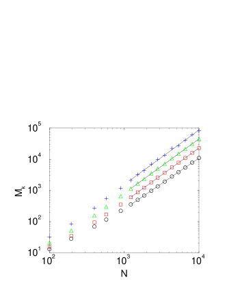
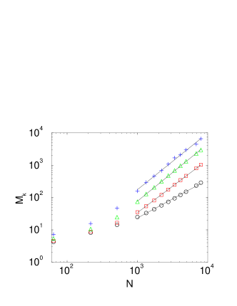
Figure 3: Double logarithmic plot of $M_{k}(N)$, the $k^{\rm th}$ reduced moments of the consensus time distribution, versus the total number of spins $N$ for $k=1$ ($\circ$), $k=2$ ($\Box$), $k=4$ ($\triangle$), $k=8$ ($+$), in $d=2$ (top) and $d=3$ (bottom). Data are based on $10^{5}$ realizations in $d=2$ and $4\times 10^{5}$ realizations in $d=3$. The lines are least-squares linear fits to the large-$N$ data.

From these data, we find that the most probable consensus time, $t_{\rm mp}$, scales with $N$ as $t_{\rm mp}\sim N^{\alpha}$, with $\alpha\approx 1.24$, $0.72$, and 0.56 for spatial dimensions 2, 3, and 4, respectively. These values are identical to those obtained previously in Ref. MM ; these were based on smaller-scale simulations in which realizations where the consensus time exceeded a (large) preset limit were terminated.

On the other hand, the asymptotic decay of $P_{N}(t)$ is clearly governed by a much longer characteristic time and we now apply two methods to estimate this longer time scale. First, we consider the reduced moments of the consensus time distribution

$$M_{k}(N)\equiv\langle(t(N))^{k}\rangle^{1/k}=\left[\int_{0}^{\infty}t^{k}\,P_{N}(t)\,dt\right]^{1/k}.$$ (1)

As suggested by the data in Fig. 2, if the long-time tail of consensus time distribution has a simple exponential decay of the form $e^{-t/\tau(N)}$ at long times, then all the reduced moments would asymptotically scale as $\tau(N)$, with subdominant corrections that become smaller as $k$ increases. This trend is illustrated in Fig. 3 where $M_{k}$ is plotted as a function of $N$ for various values of $k$. In $d=2$, each $M_{k}$ grows as a power law in $N$ for large $k$, but with a slightly different apparent exponent. Least-squares fits to the data give the following exponents in $d=2$: 1.64 for $k=1$ ($\circ$), 1.73 for $k=2$ ($\Box$), 1.75 for $k=4$ ($\triangle$), and 1.75 for $k=8$ ($+$). From this limiting large-$k$ value of this exponent we can then infer the $N$ dependence of $\tau$.

For $d=3$, the behavior is qualitatively similar, except that there is a large disparity in the exponents for $M_{k}$ for $k=1$ and for $k>1$. Linear fits to the data now give the exponent values 1.18 for $k=1$ ($\circ$), 1.64 for $k=2$ ($\Box$), 1.77 for $k=4$ ($\triangle$), and 1.78 for $k=8$ ($+$). However, there is a perceptible downward curvature in the dependence of $M_{k}$ on $N$ for large $k$, so that linear fits are inadequate to determine the $N$-dependence of $\tau$ accurately.

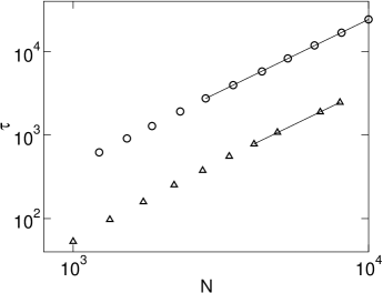
Figure 4: Double logarithmic plot of $\tau(N)$ (in units of Monte Carlo steps per spin) versus $N$ for $d=2$ ($\circ$) and $d=3$ ($\triangle$). The lines are the best fits to the last few data points.

Our second analysis method is simply to measure the slope of the exponential tail of $P_{N}(t)$ directly for different values of $N$ and thereby determine $\tau(N)$. To do this, we first make a first estimate for $\tau$ by finding the slope in the region that is visually most linear. Then we refine this estimate by computing the slopes in the systematic ranges $(\tau/2,2\tau)$, $(\tau/2,3\tau)$, $(\tau/2,4\tau)$, etc., and using the range where a linear fit has the highest correlation coefficient. In the resulting data for $\tau$ versus $N$, there is now small and systematic downward curvature (Fig. 4). By dropping the first four data points one-by-one and then performing linear fits to the remaining data, the local slope decreases from 1.746 to 1.719 in two dimensions. In three dimensions, there is a larger decrease in the local slope from 1.832 to 1.709 as the first six points are deleted. Extrapolating this local slope to $N\to\infty$, we obtain the estimates $\nu=1.7\pm 0.04$ in $d=2$ and $\nu=1.5\pm 0.1$ in $d=3$ in the relation $\tau\sim N^{\nu}$. The error bars are a subjective guess of the uncertainty in the extrapolation.

III Anomalous Coarsening and Long-Lived Coherent States

The main result of the above analysis is that the average consensus time is much larger than the dependence of $N^{2/d}$ that would arise if domain coarsening were entirely governed by diffusive dynamics. By observing the evolution of many realizations of the system, it is clear that the asymptotic tail of the consensus time distribution arises from situations where the $+$ and $-$ spins organize into spatially coherent and long-lived states that consist of relatively flat stripes in two dimensions (Fig. 5), slabs in three dimensions (Fig. 6), and analogously (we believe) in higher dimensions. The existence of these states is one of the most surprising feature of the MR model. In spite of the isotropy of the MR interaction, the long-lived transient states arise and spontaneously break this symmetry. Once the system reaches such a state, further evolution proceeds extremely slowly, as we shall discuss below.

To develop intuition for these coherent states, we show in Fig. 5 a set of snapshots of a $50\times 50$ system that happens to evolve to a stripe. After a few time steps, the lattice-scale granularity of the random initial state has disappeared due to the effective surface tension in the majority rule dynamics. After this early-time transient, the subsequent evolution qualitatively resembles the coarsening of a spin system with non-conserved order-parameter kinetics. However, domains tend to develop a stringy morphology, a feature that promotes the formation of stripes that span the system. For the realization shown, a clearly resolved stripe emerges by 100 time steps, while ultimate consensus is achieved when 1850 time steps have elapsed; notice that a time of 1850 steps is relatively early in the asymptotic tail of $P_{N}(t)$ in Fig. 2.

In spite of the anomalous long-time kinetics of the MR model, the early-time coarsening is diffusive in nature. To determine the growth of the typical domain length scale at early times, we studied the time evolution of the two-spin correlation function. We took this correlation function at different times and found the length rescaling that gave the best data collapse. We thus found that the appropriate rescaling the correlation function is by a length scale that is proportional to $t^{1/2}$. We therefore conclude that the early-time coarsening in the MR model is characterized by a length scale that grows as $t^{1/2}$.

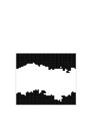
Figure 5: Snapshots of a $50^{2}$ system at $t=0,1,5,20,80$, & 200.

A phenomenon analogous to stripe formation occurs in three dimensions, where long-lived states arise that consist of two relatively flat slabs of oppositely-oriented spins (Fig. 6). For the example shown from a $20^{3}$ lattice, a slab state forms around 150 time steps, while final consensus does not occur until 3800 time steps have elapsed.

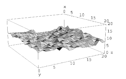
Figure 6: One of the two interfaces of the slab state on a cubic lattice of linear dimension $20$. Coordinates are in units of lattice spacing.

To verify that stripe states actually govern the asymptotic tail of $P_{N}(t)$ two dimensions, we also study the evolution of a synthetic system with an ordered initial state that consists of two straight stripes, with half the spins $+$ and half the spins $-$. The long-time tail of the consensus time distribution for this special initial condition follows a single exponentially decaying function, as shown in Fig. 7. Also shown in this figure is the corresponding distribution for a system of the same size with a random zero-magnetization initial condition. The coincidence of the slopes in the tails of these two distributions shows that stripe states control the long-time evolution of random zero-magnetization initial condition systems.

Because of the crucial role that spatially coherent states play in the MR model, we also study the probability $S_{N}(m)$ that a randomly-prepared $N$-spin system in $d$ dimensions with initial magnetization $m$ evolves to such a state. We use two independent methods to measure $S_{N}(m)$. One is based on simply counting the fraction of realizations whose consensus time lies within the asymptotic tail of the consensus time distribution. For example, for the data from the $50\times 50$ system in Fig. 2, the tail region corresponds to a consensus time $t$ greater than 600. Thus for this system size all realizations with $t>600$ are counted as reaching a coherent state.

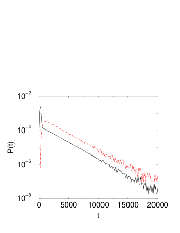
Figure 7: Consensus time distribution for a $50^{2}$ square lattice for a two-stripe (dashed) and random initial condition (solid). All data are based on $10^{5}$ realizations. Time is in units of Monte Carlo steps per spin.

Alternatively, we investigate correlation functions that are engineered to detect stripe states. For $d=2$, we consider the following correlation functions for two spins that are located a distance $L/2$ apart:

$$C_{x}(t) \equiv \frac{1}{2}\langle s(x,y,t)s(x\pm L/2,y,t)\rangle,$$

$$C_{y}(t) \equiv \frac{1}{2}\langle s(x,y,t)s(x,y\pm L/2,t)\rangle.$$

For both a random state and for consensus, these correlation functions equal zero. Conversely, for an ordered two-stripe state with stripes of width $L/2$ parallel to the $x$-axis, $C_{x}=+1$ and $C_{y}=-1$, and vice versa for stripes parallel to the $y$-axis. We therefore posit that a stripe state arises if the correlation function in the direction(s) parallel to the stripe is greater than a threshold value, while the correlation function perpendicular to the stripe is less than the negative of this threshold value. We arbitrarily choose the threshold to equal 0.5, but our results for large $N$ depend only weakly ($S_{N}(m=0)$ varies by $\leq 10\%$) on the threshold value when it is in the range 0.3 – 0.7. The results given below are based on the threshold set to 0.5.

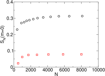
Figure 8: Probability to reach a stripe state versus number of spins $N$ for $d=2$ ($\circ$) and $d=3$ ($\Box$) using the threshold value 0.5 (see text). Data are based on $10^{5}$ realizations.

We find that the stripe/slab probability $S_{N}(m=0)$ grows quickly for small $N$ and then saturates to a non-zero value that is close to 0.33 in $d=2$ and 0.08 for $d=3$ (Fig. 8). The stripe probability in two dimensions is very close to that found previously in the zero-temperature evolution of the Ising model with Glauber kinetics SKR . Note also that as the initial magnetization $m$ is moved away zero, $S_{N}(m)$ quickly decays to zero (Fig. 9). This simply reflects the fact that if one phase is initially below the percolation threshold, there is a very small possibility for minority phase droplets to merge and form a stripe that spans the system.

Figure 9: Probability to reach a stripe state versus initial magnetization $m$ for a $50^{2}$ system. Data are based on $10^{5}$ realizations.

We can qualitatively understand the dimension dependence of the probability to reach a stripe state by the following rough argument (see also Ref. SKR ). For simplicity, we first discuss the case of two dimensions with the random zero-magnetization initial condition. Consider a large system of linear dimension $L$ and cut it into four equal subsquares of linear size $L/2$. The final state in each of these subsquares is reached more quickly than that of the entire system. We now make the plausible assumption, based on observations of many realizations of the system, that each subsquare independently reaches consensus. Then out of the $2^{4}$ possible configurations of these subsquares, only the following arrangements

$$\begin{array}[]{llll}~{}~{}++&~{}~{}--&~{}~{}+-&~{}~{}-+\\ ~{}~{}--&~{}~{}++&~{}~{}+-&~{}~{}-+,\end{array}$$

where the $+$ and $-$ symbols refer to the final state of each subsquare, correspond to a stripe state of the $L\times L$ system. This argument then suggests that $S_{N}(m=0)=4/2^{4}=1/4$.

This coarse-graining argument straightforwardly generalizes to higher spatial dimensions. On the cubic lattice, we divide an $L\times L\times L$ cube into eight subcubes of linear dimension $L/2$. If these subcubes each independently reach consensus, then a slab state on the original cube (consisting of two slabs of oppositely oriented spins, each of size $L\times L\times L/2$) can be achieved in six possible ways. The probability of reaching a slab state is therefore $6/2^{8}\approx 0.047$. In $d$ dimensions, this same line of reasoning gives $S_{N}(m=0)=2d/2^{2^{d}}$. While our argument is crude, the resulting numerical values for $S_{N}$ qualitatively mirror the corresponding estimates from simulations.

Our approach also helps explain why stripe states quickly disappear when the initial magnetization is non-zero. As an example, for initial magnetization 0.08, we find by numerical simulations that the probability that a $25\times 25$ system eventually ends with all spins $+$ is 0.88. Now employing the above coarse-graining argument for a $50\times 50$ system, the four $25\times 25$ subsquares will each reach $+$ consensus with probability 0.88 and $-$ consensus with probability 0.12. Then the probability for the $50\times 50$ system to reach a stripe state is $S_{N}\approx 4(0.88)^{2}\,(0.12)^{2}\approx 0.0446$. This is very close (probably fortuitously) with our numerical result of $S_{N}(m=0.08)\approx 0.0498$.

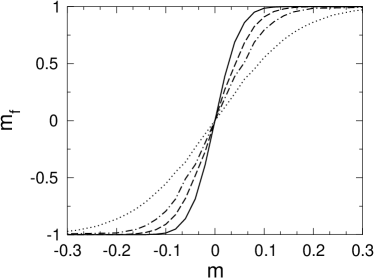
Figure 10: Final magnetization $m_{f}$ as a function of initial magnetization $m$, on the square lattice for linear dimension $L=10$ (dotted curve), 20 (dashed), 30 (dot-dash), and 50 (solid).

Another important aspect of the evolution to the final state is the dependence of the final magnetization on the initial magnetization. Since the system always reaches consensus, the final magnetization $m_{f}$ is simply the difference in the probabilities that the systems ends with all spins $+$ and all spins $-$. On the square lattice, we find that the curve of the final magnetization versus the initial magnetization approaches a step function as $N\to\infty$ (Fig. 10). Thus any initial bias pre-determines the final state of the system in the thermodynamic limit. This step-function behavior is in contrast to the behavior in one dimension, where the final magnetization curve remains non-singular as $N\rightarrow\infty$ MM . Finally, it is worth noting that $m_{f}$ equals the initial magnetization $m$ for the voter model in all spatial dimensions voter ; there is no tyranny of the majority in the voter model.

IV Lifetime of Stripe States

Once a stripe state is formed, the evolution to ultimate consensus is controlled by the time required for the two interfaces that define the stripe to meet and annihilate. In one dimension, it is easy to see that each isolated interface between $+$ and $-$ spins moves by free diffusion. When two interfaces approach to nearest-neighbor separation they necessarily annihilate. (Note that in the kinetic Ising model, two nearest-neighbor interfaces can annihilate, with probability 1/2, or recede by one lattice spacing, also with probability 1/2, in a single update step.)  Therefore the time for the last two domain walls to annihilate is proportional to $L^{2}$, where $L$ is the linear dimension of the system. Further, because the system is controlled by the meeting of two random walks on a finite ring, the consensus time distribution has an exponential decay of the form $e^{-t/N^{2}}$ fpp .

In two and three dimensions, the interfaces between stripes are quite smooth (Figs. 5 & 6) and the scaling of the interface width on the transverse dimension of the system appears to be in the Edwards-Wilkinson universality class BS . We verified the smoothness of the interface by preparing a system of linear size ${\cal L}\times L^{(d-1)}$ in $d$ dimensions, with ${\cal L}\gg L$, in which all spins in the region $[0,{\cal L}/2]$ are initially in the $-$ state, and all spins in the region $[{\cal L}/2,{\cal L}]$ are initially in the $+$ state. In two dimensions, the width $w$ of the interface initially grows slowly in time and eventually saturates to a value that approximately scales as $w\sim L^{1/2}$. In three dimensions, the growth of the width is even slower and the saturation value of the width is consistent with a logarithmic dependence on $L$.

Thus it is the diffusion of the interface as a whole rather than fluctuations in the interface shape that determines the lifetime of the stripe state. Since the interfaces are typically separated by a distance of order $L$ when they are first formed, the lifetime $T$ of the stripe state should therefore given by

$$T\sim\frac{L^{2}}{D(L)},$$ (3)

where $D(L)$ is the diffusion coefficient of a single interface with transverse dimension $L$.

We may obtain a simple albeit rough estimate for this diffusion coefficient by treating each site on the interface as an independent random walk SKR ; PRL . For a $d$-dimensional system, a smooth interface contains of the order of $L^{d-1}$ sites. In a single time step, each interface site will randomly move by $\pm 1$ perpendicular to the interface. Hence if each site is independent, the center of mass of the interface will move by a distance $\sqrt{L^{d-1}}/L^{d-1}\sim L^{-(d-1)/2}$ in one time step. As a result, the diffusion coefficient of the interface $D(L)$ scales as $L^{-(d-1)}$.

We tested this prediction by simulation by following the evolution of a single interface in a long strip (or slab) geometry with transverse dimension $L$ in which all the spins on the right half are set to $+1$ and all the spins on the left half are set to $-1$. We then let the spins evolve by majority rule dynamics. After a short transient that lasts of the order of one time step, we observe that the interface moves diffusively, with a diffusion coefficient that scales approximately as $L^{-1}$ in two dimensions and as $L^{-2}$ in three dimensions. Given the crudeness of the above random walk argument, it is surprising that the simulation results agree quite well with the prediction $D(L)\sim L^{-(d-1)}$.

From this scaling of the diffusion coefficient on the transverse linear dimension $L$, Eq. (3) then gives a consensus time $T$ that scales as $T\sim L^{d+1}$. Equivalently, in terms of the total number of spins $N=L^{d}$, the dependence is $T\sim N^{(d+1)/d}$. However, this prediction is only qualitatively consistent with the exponent values of $1.7$ for $d=2$ and $1.5$ for $d=3$ that were obtained from direct numerical simulations of the consensus time distribution. We do not have an explanation for this discrepancy.

V Summary and Discussion

We studied the time evolution of the majority rule (MR) model for finite-dimensional systems. One of our main results is that the approach to consensus in an initially unbiased system is surprisingly complex. Before ultimate consensus is reached, a non-trivial fraction of all realizations falls into coherent metastable states that consist of stripes in two dimensions and slabs in three dimensions. We anticipate that analogous coherent states arise in higher spatial dimensions. The interfaces between domains in these coherent states are quite smooth and reflect the strong surface tension in the majority rule dynamics.

Due to these coherent states, the time to reach consensus is anomalously long and is controlled by a diffusion process that brings two interfaces close enough that they can annihilate. The characteristic time scale for this annihilation is much longer than the most probable time to reach consensus. The fraction of realizations that reach these long-lived states decreases as $d$ increases, but their role appears to be dominant in the asymptotic kinetics. When the initial magnetization is non-zero, however, these long-lived states quickly disappear. As a result, the consensus time distribution has a single peak and there is no long-time tail. Furthermore, the time until consensus grows only logarithmically in the system size (Fig. 11). Thus an initial bias in the density of spins is a decisive influence in the long-time behavior of the system.

Figure 11: Consensus time (in units of Monte Carlo steps per spin) versus $N$ in $d=2$ for initial magnetization $m=0.2$.

We gave a crude coarse-graining argument to estimate the probability to reach a coherent state as a function of the spatial dimension. This approach qualitatively explained the behavior of the probability to reach such a state as a function of the spatial dimension $d$ and the initial magnetization.

Finally, we suggest several directions for further study. First, it would be worthwhile to determine the value of the upper critical dimension of the MR model. An exact analysis of this model on the complete graph, where all spins are nearest neighbors of each other, showed that the mean consensus time grows as $\ln N$ MM . On the other hand, the simulations presented here and in MM suggested that the mean consensus time grows as a power law in $N$ for spatial dimensions 1, 2, 3, and 4. These two facts suggest that the upper critical dimension of the MR model is greater than 4. It would be worthwhile to have a theoretical understanding for the apparently large value of the upper critical dimension.

We also believe it will be fruitful to study simple extensions of the MR model with more stringent conditions for achieving consensus. One example is to have a higher threshold than simple majority before the opinion of a group is swayed. While a higher threshold will obviously slow the dynamics, it should be interesting to investigate whether this modification leads to different scaling properties for the mean consensus time and the distribution of consensus times.

A more intriguing generalization arises when each spin has more than two opinions, where we anticipate new types of dynamical behavior. With more than two states, the possibility of a dynamically-stable steady state that consists of coalescing and coexisting multiple opinion groups was discussed in the framework of the “stochastic seceder” model SH03 . In the context of our majority rule model, there obviously will be slower dynamics because it may be possible to have a group with no local majority, but only a local plurality. Such a group would not evolve according to the majority rule dynamics. Thus configurations in which there is no majority in each group represent another absorbing state for the dynamics. In the mean-field limit, we find that such a system never reaches this frustrated state, as the corresponding fixed point of equal concentrations of all species is unstable CR . Instead, for a system with more than two opinion states, the time to reach ultimate consensus is merely increased by a multiplicative factor compared to the two-opinion MR model. However, for finite spatial dimensions, the existence of more than two opinions appears to have a more significant effect on the long-time behavior that depends fundamentally on the interplay between the group size and the number of states. When there are many distinct local majorities in the initial state the group dynamics has a primarily diffusive character. However, when there is of the order of one local majority, the opinion of this group quickly overtakes the entire system.

VI Acknowledgments

We thank Pablo Hurtado, Paul Krapivsky, Mauro Mobilia, and Federico Vazquez for helpful discussions and advice. We also thank NSF grant DMR0227670 for financial support of this research.

References

- (1) S. Galam, Physica (Amsterdam) 274, 132 (1999); Eur. Phys. J. B 24, 403 (2002); cond-mat/0211571.
- (2) P. L. Krapivsky and S. Redner, Phys. Rev. Lett. 90, 238701 (2003).
- (3) F. Slanina and H. Lavicka, Eur. Phys. J. B 35, 279 (2003).
- (4) T. M. Liggett, Interacting Particle Systems (Springer-Verlag, New York, 1985).
- (5) R. J. Glauber, J. Math. Phys. 4, 294 (1963).
- (6) P. L. Krapivsky, Phys. Rev. A 45, 1067 (1992).
- (7) S. Redner, A Guide to First-Passage Properties, (Cambridge University Press, New York, 2001).
- (8) J. D. Gunton, M. San Miguel, and P. S. Sahni in: Phase Transitions and Critical Phenomena, Vol. 8, eds. C. Domb and J. L. Lebowitz (Academic, NY 1983); A. J. Bray, Adv. Phys. 43, 357 (1994).
- (9) K. Sznajd-Weron and J. Sznajd, Int. J. Mod. Phys. C 11, 1157 (2000); D. Stauffer, J. Artif. Soc. Soc. Simul. 5, no. 1 (2002).
- (10) V. Spirin, P. L. Krapivsky, and S. Redner, Phys. Rev. E 63, 036118 (2001); Phys. Rev. E 65, 016119 (2002).
- (11) See e.g., A.-L. Barabási and H. E. Stanley, Fractal Concepts in Surface Growth, (Cambridge University Press, Cambridge, 1995).
- (12) M. Plischke, Z. Rácz, and D. Liu, Phys. Rev. B 35, 3485 (1987).
- (13) A. Soulier and T. Halpin-Healy, Phys. Rev. Lett. 90 258103 (2003).
- (14) P. Chen and S. Redner, in preparation.