Asymptotics of superstatistics

Abstract

Superstatistics are superpositions of different statistics relevant for driven nonequilibrium systems with spatiotemporal inhomogeneities of an intensive variable (e.g., the inverse temperature). They contain Tsallis statistics as a special case. We develop here a technique that allows us to analyze the large energy asymptotics of the stationary distributions of general superstatistics. A saddle-point approximation is developed which relates this problem to a variational principle. Several examples are worked out in detail.

I Introduction

Many driven nonequilibrium systems exhibit complex dynamical behavior characterized by spatiotemporal fluctuations of an intensive parameter $\beta$ which may represent an inverse temperature, a chemical potential (e.g., in a system with inhomogeneous concentrations), an effective friction constant, the amplitude of a perturbing noise, or the local energy dissipation, as in the case of turbulent flows. Although such systems do not settle to equilibrium, their long-term behavior can often be described in the spirit of equilibrium statistical mechanics by viewing them as consisting of an ensemble of subsystems or “cells” to which are associated different values of $\beta$. If there is local equilibrium in each cell, so that statistical mechanics can be applied locally, and if the fluctuations of $\beta$ evolve on a sufficiently large time scale, then in the long-term run the entire system can be described by a mixture or superposition of different Boltzmann factors having different values of $\beta$. Such a mixture of various statistics has been termed a “superstatistics” beck-cohen and has been the subject of various papers lately (see, e.g., Refs. cohen ; boltzmann-m ; beck-su ; touchette ; sattin04 ; supergen ; abestab ; abearbi ; souza ; souza2 ; luczka2000 ). Many models based on the notion of superstatistics have also been applied successfully to a variety of physical problems, including Lagrangian beck03 ; reynolds03 and Eulerian turbulence old-physica-d ; beck-physica-d , defect turbulence daniels , cosmic ray statistics beck-physica-a , plasmas sattin02 , statistics of wind velocity differences rapisarda , and econophysics ausloos ; econo .

What is common to all these problems is the experimental observation of stationary distributions having “fat” tails. Such distributions fall necessary outside the framework of ordinary statistical mechanics, but not that of superstatistics. For example, if the random intensive parameter $\beta$ in the various cells is taken to be distributed according to a particular probability distribution, the $\chi^{2}$-distribution, then the corresponding superstatistics, obtained by integrating the Boltzmann factor $e^{-\beta E}$ over all $\beta$, yields the nonextensive statistics of Tsallis defined by the so-called $q$-exponential function tsa1 ; tsa2 ; tsa3 ; abe

$$e_{q}^{-\beta_{0}E}=[1+(q-1)\beta_{0}E]^{-1/(q-1)}.$$ (1)

This particular statistics decays as a power-law for large energies $E$ rather than an exponential, as is the case for the ordinary Boltzmann factor. In this sense, it is a fat-tailed statistics. The parameter $\beta_{0}$ above is related in the superstatistical model to the average inverse temperature of the inhomogeneous system, whereas the so-called entropic index $q$ relates to the variance of the $\beta$ fluctuations wilk ; prl . It is worth mentioning that distributions having the form of a $q$-exponential can be obtained formally by maximizing Tsallis’ measure of entropy subject to suitable constraints. Moreover, ordinary statistical mechanics, which correspond in the superstatistics picture to the case where there is no fluctuations in $\beta$, is recovered in the limit where $q\to 1$ tsa1 ; tsa2 ; tsa3 ; abe .

For other distributions of the intensive parameter $\beta$, one ends up with more general superstatistics. Generalized entropies, which are analogs of the Tsallis entropies, can also be defined for these general superstatistics abearbi ; souza , and generalized versions of statistical mechanics can be constructed, at least in principle. It has been shown that the corresponding generalized entropies are stable abestab ; souza2 .

In this paper we will briefly review the superstatistics concept, and then analyze the asymptotic behavior of general superstatistics for large values of the energy $E$. We will investigate how the properties of the function $f(\beta)$, which represents the probability distribution of the intensive variable $\beta$ in the various spatial cells, determine the asymptotic decay rate of the generalized Boltzmann factor of the superstatistics. We develop a saddle-point approximation technique which allows us to treat this problem in full generality. Several examples will be worked out in detail to show that the asymptotic decay rate of the stationary distributions resulting from $f(\beta)$ can not only be a power-law, as in the case of nonextensive statistics, but can also be an exponential of the square root of the energy or, generally, a stretched exponential. We will discuss universal aspects of the large energy asymptotics, thus complementing the consideration in Ref. beck-cohen where universal aspects of the low-energy behavior of general superstatistics were discussed. The large energy asymptotics is of particular physical importance because the tails of the observed distributions measured in various experiments (e.g., hydrodynamic turbulence bodenschatz04 , plasmas carbone2000 , and granular media vanzon2004 ) can distinguish between the various possible types of superstatistics.

II Superstatistics: basic concept

Let us first briefly review the superstatistics concept as introduced in Ref. beck-cohen . Consider a driven nonequilibrium system with spatiotemporal fluctuations of an intensive parameter $\beta$, for example, the inverse temperature. Locally, i.e., in spatial regions (cells) where $\beta$ is approximately constant, the system is described by ordinary statistical mechanics, i.e., by an ordinary Boltzmann factor $e^{-\beta E}$, where $E$ is an effective energy in each cell. In the long-term run, the system is described by a spatiotemporal average over the fluctuating $\beta$. In this way, one may define an effective Boltzmann factor $B(E)$ for the whole system as

$$B(E)=\int_{0}^{\infty}f(\beta)e^{-\beta E}d\beta=\langle e^{-\beta E}\rangle,$$ (2)

where $f(\beta)$ is the normalized probability distribution describing the $\beta$-fluctuations in the various cells. For so-called type-A superstatistics, one normalizes this effective Boltzmann factor and obtains the stationary, long-term probability distribution,

$$p(E)=\frac{1}{Z}B(E),$$ (3)

where

$$Z=\int_{0}^{\infty}B(E)dE.$$ (4)

For type-B superstatistics, the $\beta$-dependent normalization constant of each local Boltzmann factor is included into the averaging process. In this case, the invariant long-term distribution is given by

$$p(E)=\int_{0}^{\infty}f(\beta)\frac{e^{-\beta E}}{Z(\beta)}d\beta,$$ (5)

where $Z(\beta)$ is the normalization constant of the Boltzmann factor $e^{-\beta E}$ for a given $\beta$. Both approaches can be easily mapped into each other by considering a new probability density $\tilde{f}(\beta)=c\cdot f(\beta)/Z(\beta)$, where $c$ is a normalization constant. One immediately recognizes that type-B superstatistics with $f$ is equivalent to type-A superstatistics with $\tilde{f}$.

As mentioned before, the fluctuations of the intensive parameter $\beta$ are spatiotemporal: they can be produced by either temporal changes of the environment or by the movement of a test particle through inhomogeneous spatial regions. The precise nature and behavior of $\beta$ in these situations can be quite varied. In our general description of superstatistics, we have taken $\beta$ to be an inverse temperature which varies randomly in time or in space, but $\beta$ can also represent, say, a chemical potential that varies smoothly in space. In this way, one may study superstatistical models where the fluctuations of $\beta$ are caused by large-scale temperature gradients in a system sattin04 or by a nonuniform chemical potential describing inhomogeneous concentrations spread in space.

From a more dynamical perspective, a superstatistics can also be achieved by considering Langevin equations whose parameters fluctuate on a relatively large time scale (the adiabatic regime note1 ); see Ref. prl for details. For turbulence applications, for example, one may consider a superstatistical extension of the Sawford model of Lagrangian turbulence beck03 ; reynolds03 ; sawford . This model consists of suitable stochastic differential equations for the position, velocity, and acceleration of a Lagrangian test particle in the turbulent flow. The superstatistical extension naturally enters due to the fact that the local energy dissipation rate in turbulent flows is a random variable. Thus the parameters of the Sawford model become random variables as well. These kinds of models well reproduce experimentally measured turbulence data beck03 ; reynolds03 .

In the following we will use the notation of type-A superstatistics, keeping in mind that we can always proceed to type-B superstatistics by replacing $f$ by $\tilde{f}$. We will restrict ourselves to positive values of $\beta$ and $E$ and will assume, in addition, that $f(\beta)$ is everywhere differentiable and unimodal (single-bell-shaped curve).

III Low energy asymptotics

We recall the low-energy asymptotics of superstatistics for reasons of completeness; it was previously discussed in Ref. beck-cohen . Consider a distribution $f(\beta)$ having mean $\left\langle\beta\right\rangle=\beta_{0}$ and variance

$$\left\langle\beta^{2}\right\rangle-\left\langle\beta\right\rangle^{2}=\left\langle\beta^{2}\right\rangle-\beta_{0}^{2}=\sigma^{2}.$$ (6)

Using the definition of $B(E)$, we can write

$$B(E)=\left\langle e^{-\beta E}\right\rangle=e^{-\beta_{0}E}\left\langle e^{-(\beta-\beta_{0})E}\right\rangle.$$ (7)

Then, expanding in Taylor series the exponential term inside the expected value, we obtain

$$B(E)=e^{-\beta_{0}E}\left(1+\frac{1}{2}\sigma^{2}E^{2}+\sum_{k=3}^{\infty}\left\langle(\beta_{0}-\beta)^{k}\right\rangle\frac{E^{k}}{k!}\right).$$ (8)

Thus, to second order in $E$, $B(E)$ must behave like

$$B(E)\sim e^{-\beta_{0}E}\left(1+\frac{1}{2}\sigma^{2}E^{2}\right)$$ (9)

as $E\rightarrow 0$. This approximation represents the leading order correction to ordinary statistical mechanics in our nonhomogeneous system with temperature fluctuations for small values of the energy $E$. The zeroth-order approximation to $B(E)$ corresponds, as is expected, to the “pure” Boltzmann statistics,

$$B(E)\sim e^{-\beta_{0}E},$$ (10)

with inverse temperature $\beta_{0}$. It can be noted that these two asymptotic results can also be considered to be valid approximations of $B(E)$ in the limit where $\left\langle(\beta_{0}-\beta)^{k}\right\rangle\rightarrow 0$ for all $k\geq 2$, that is essentially when $f(\beta)\rightarrow\delta(\beta-\beta_{0})$ (small fluctuations limit).

IV High energy asymptotics

To find the high-energy asymptotics of $B(E)$, we use the fact that the integral defining $B(E)$ has the form of a Laplace integral for $E\rightarrow\infty$ bender1978 . In this limit, the integral can be approximated by its largest integrand. This is the essence of Laplace method, otherwise known as the saddle-point approximation bender1978 ; murray1984 . The conditions of applicability of this approximation method are basically the conditions that we have assumed regarding the shape of $f(\beta)$ and its differentiability. Thus, putting $B(E)$ in the form

$$B(E)=\int_{0}^{\infty}e^{-\beta E+\ln f(\beta)}d\beta,$$ (11)

we attempt to locate the largest integrand by finding the unique value of $\beta$ which maximizes the exponent function,

$$\Phi(\beta,E)=-\beta E+\ln f(\beta),$$ (12)

for any large enough energy value $E$. We call the value of $\beta$ maximizing $\Phi(\beta,E)$ for fixed $E$ the dominant inverse temperature and denote it by $\beta_{E}$. The fact that $f(\beta)$ is assumed to be unimodal ensures us that $\beta_{E}$ is unique, as required. Indeed, observe that $\ln f(\beta)$ must be a concave function of $\beta$ if $f(\beta)$ is unimodal (see Fig. 1), and, in this case, the maximum of $\Phi(\beta,E)$ along the $\beta$-direction can only be attained at a single point $\beta_{E}$ which is such that

$$E=[\ln f(\beta)]^{\prime}=\frac{f^{\prime}(\beta)}{f(\beta)}.$$ (13)

Solving this equation for $\beta$, we find $\beta_{E}$ and thus write

$$B(E) \sim e^{\Phi(\beta_{E},E)}$$ (14)

$$= e^{-\beta_{E}E+\ln f(\beta_{E})}$$

$$= f(\beta_{E})e^{-\beta_{E}E}$$

in the limit where $E\rightarrow\infty$. Note that this basic Laplace or saddle-point approximation of $B(E)$ can be improved a bit more by evaluating the integral defining $B(E)$ using a Gaussian approximation of the integrand bender1978 . What results from this more refined approximation is the following high-energy asymptotics:

$$B(E)\sim\frac{f(\beta_{E})e^{-\beta_{E}E}}{\sqrt{-[\ln f(\beta_{E})]^{\prime\prime}}}$$ (15)

which differs from the Laplace approximation only by the square-root term involving the curvature of $\ln f(\beta)$.

The Laplace approximation of $B(E)$ as well as its Gaussian corrected version shown above are quite interesting from the physical point of view because they show that the mixture of Boltzmann statistics defining $B(E)$ reduces at high energy $E$ to a “pure” Boltzmann statistics, just like in the equilibrium situation, although now the Boltzmann statistics involves an inverse temperature $\beta_{E}$ which depends on the energy $E$ considered. This means that, for high values of $E$, the long-term, stationary behavior of the nonequilibrium system considered is dominated by the equilibrium behavior of a subset of cells having an inverse temperature equal or close to $\beta_{E}$. How $\beta_{E}$ changes as a function of $E$ is determined from the properties of $f(\beta)$. In the general case considered here, where $\ln f(\beta)$ concave, we find that $\beta_{E}\rightarrow 0$ when $E\rightarrow\infty$ (see Fig. 1). Thus in this case the large-energy behavior of the generalized Boltzmann factors $B(E)$ is determined by the small-$\beta$ (high temperature) behavior of the function $f(\beta)$.

To complete this section, note that the exponent function $\Phi(\beta_{E},E)$ which enters in the asymptotics of $B(E)$ represents nothing but the Legendre transform of $\ln f(\beta)$. The result of this transform is a function of $E$ which can be thought of to represent, following the theory of large deviations ellis1985 , an entropy function if we consider that the function $\ln f(\beta)$ represents a free energy function. This entropy function, however, is just a formal one and is unrelated to the Tsallis entropies or other generalized entropies as defined in Refs. tsa1 ; souza .

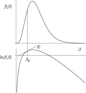
Figure 1: Plot of a typical unimodal distribution $f(\beta)$ (top) and its logarithm (bottom). The dominant inverse temperature $\beta_{E}$ is such that $\ln f(\beta_{E})$ has a slope equal to the energy value $E$.

V Examples

We now consider a few cases of $\beta\rightarrow 0$ asymptotic behavior of $f(\beta)$ and derive the corresponding asymptotic behavior of $B(E)$ for $E\rightarrow\infty$ using the Laplace approximation of $B(E)$ corrected with the square-root term, i.e., Eq.(15).

V.1 Power-law tail

Consider first an $f(\beta)$ with $f(\beta)\sim\beta^{\gamma}$, $\gamma>0$ for $\beta\to 0$. An example of probability density having this asymptotic form is the following $\chi^{2}$ distribution for $\beta$ prl ; wilk :

$$f(\beta)=\frac{1}{\Gamma(\frac{n}{2})}\left(\frac{n}{2\beta_{0}}\right)^{n/2}\beta^{n/2-1}e^{-\frac{n\beta}{2\beta_{0}}},$$ (16)

($\beta_{0}\geq 0$, $n>1$), which behaves as $f(\beta)\sim\beta^{n/2-1}$ around $\beta=0$. Another example is the $F$-distribution beck-cohen ; sattin02 ,

$$f(\beta)=C\frac{\beta^{\frac{v}{2}-1}}{(1+\frac{vb}{w}\beta)^{(v+w)/2}},$$ (17)

where $v,w,b$ are parameters and $C$ is a normalization constant.

To find the asymptotic form of the superstatistics $B(E)$ corresponding to the choice $f(\beta)\sim\beta^{\gamma}$, we proceed to determine the value of the dominant inverse temperature $\beta_{E}$ by solving Eq.(13). The solution here is $\beta_{E}=\gamma/E$, so that

$$-\beta_{E}E+\ln f(\beta_{E}) = -\gamma+\gamma\ln\gamma-\gamma\ln E$$ (18)

$$\sim -\gamma\ln E$$

and

$$[\ln f(\beta_{E})]^{\prime\prime}=-\frac{\gamma}{\beta_{E}^{2}}=-\frac{E^{2}}{\gamma}\sim-E^{2}.$$ (19)

Combining the two results in (14), we obtain

$$B(E)\sim\frac{e^{-\gamma\ln E}}{E}=E^{-\gamma-1}.$$ (20)

Thus we see that power laws in $\beta$ for small $\beta$ imply a power law in $E$ for large $E$, no matter what the rest of the distribution $f(\beta)$ looks like. Comparing this asymptotic result with the $q$-exponential distributions studied in nonextensive statistical mechanics tsa1 ; tsa2 ; tsa3 ; abe , which asymptotically decay as $E^{-1/(q-1)}$, we see that

$$\gamma+1=\frac{1}{q-1}.$$ (21)

Power-law superstatistics are physically relevant for many different physical problems: e.g., defect turbulence daniels , cosmic ray statistics beck-physica-a , and wind velocity measurements rapisarda among others.

V.2 Exponential tail

Consider now a density $f(\beta)$ having the asymptotic form $f(\beta)\sim e^{-c/\beta}$, $c>0$, as $\beta\rightarrow 0$. An example is the inverse $\chi^{2}$ distribution

$$f(\beta)=\frac{\beta_{0}}{\Gamma(\frac{n}{2})}\left(\frac{n\beta_{0}}{2}\right)^{n/2}\beta^{-n/2-2}e^{-\frac{n\beta_{0}}{2\beta}},$$ (22)

($\beta_{0}>0$, $n>1$), which behaves, for $\beta\rightarrow 0$, as follows:

$$f(\beta)\sim\beta^{-n/2-2}e^{-\frac{n\beta_{0}}{2\beta}}\sim e^{-\frac{n\beta_{0}}{2\beta}}.$$ (23)

This form of $f(\beta)$ was previously considered in the context of density fluctuations in fusion plasma experiments sattin02 as well as temperature fluctuations in perfect gases touchette , and arises if the temperature $T=(k_{B}\beta)^{-1}$ rather than $\beta$ itself is $\chi^{2}$-distributed.

For this example, the equation that we need to solve to find $\beta_{E}$ is simply

$$[\ln f(\beta)]^{\prime}=\frac{c}{\beta^{2}}=E,$$ (24)

and so $\beta_{E}=\sqrt{c/E}$. As a result,

$$-\beta_{E}E+\ln f(\beta_{E})=-2\sqrt{cE}$$ (25)

and

$$B(E)\sim\frac{e^{-\beta_{E}E+\ln f(\beta_{E})}}{\sqrt{-[\ln f(\beta_{E})]^{\prime\prime}}}\sim E^{-3/4}e^{-2\sqrt{cE}}$$ (26)

using the fact that

$$[\ln f(\beta_{E})]^{\prime\prime}=-\frac{2c}{\beta_{E}^{3}}=-\frac{2E^{3/2}}{c^{1/2}}\sim-E^{3/2}.$$ (27)

Here the effective Boltzmann factor $B(E)$ decays as an exponential of $\sqrt{E}$. In particular, if $E=\frac{1}{2}u^{2}$ is a kinetic energy, one obtains distributions that exhibit exponential tails in the velocity $u$ touchette . This type of exponential behavior has been observed for stationary distributions of the complex Ginzburg Landau equation chate , as well as in fusion plasma experiments sattin02 .

V.3 Stretched exponential tail

As a generalization of the previous example, consider a density $f(\beta)$ which behaves as $f(\beta)\sim e^{-c\beta^{\delta}}$, with $c>0$, $\delta<0$ as $\beta\to 0$. This particular form of stretched exponential implies a high-energy behavior of $B(E)$ which also has the form of a stretched exponential. Indeed, solving the differential equation satisfied by $\beta_{E}$:

$$[\ln f(\beta)]^{\prime}=-c\delta\beta^{\delta-1}=c|\delta|\beta^{\delta-1}=E,$$ (28)

we find

$$\beta_{E}=\left(\frac{E}{c|\delta|}\right)^{1/(\delta-1)}.$$ (29)

With this value of $\beta_{E}$, the curvature of $\ln f(\beta)$ is asymptotically evaluated as follows:

$$[\ln f(\beta_{E})]^{\prime\prime} = -c\delta(\delta-1)\beta_{E}^{\delta-2}$$ (30)

$$= -c\delta(\delta-1)\left(\frac{E}{c|\delta|}\right)^{(\delta-2)/(\delta-1)}$$

$$\sim -E^{(\delta-2)/(\delta-1)}.$$

Similarly, the Legendre transform of $\ln f(\beta)$ is found to behave as

$$-\beta_{E}E+\ln f(\beta_{E}) = \frac{E^{\delta/(\delta-1)}}{(c|\delta|)^{1/(\delta-1)}}-\frac{c}{(c|\delta|)^{\delta/(\delta-1)}}E^{\delta/(\delta-1)}$$ (31)

$$= \frac{E^{\delta/(\delta-1)}}{(c|\delta|)^{1/(\delta-1)}}\left(1-\frac{1}{|\delta|}\right)$$

$$= aE^{\delta/(\delta-1)}$$

as $E\rightarrow\infty$. From Eq.(15), we consequently obtain

$$B(E)\sim E^{(2-\delta)/(2\delta-2)}e^{aE^{\delta/(\delta-1)}}.$$ (32)

Stretched exponentials are relevant for observed distributions in hydrodynamic turbulence bodenschatz04 , plasma experiments carbone2000 , as well as in granular media vanzon2004 . It is worth pointing out that the idea of superposing exponential factors to obtain a stretched exponential factor has been used previously by Palmer et al. palmer1984 to model anomalous relaxation dynamics; see also jou1990 for applications of the same idea in the context of dissipative fluxes dynamics.

V.4 Constant tail

So far we have assumed that $f(\beta)\rightarrow 0$ as $\beta\rightarrow 0$. We next consider a case where $f(\beta)$ goes to some constant as $\beta\rightarrow 0$. For this case, the differential equation defining $\beta_{E}$ poses a problem because $[\ln f(\beta)]^{\prime}$ does not diverge as $\beta$ approaches $0$. To define $\beta_{E}$, we must then resort to find the largest value of $\Phi(\beta,E)$ directly without the use of derivatives. As an example, consider the case where the $\beta\to 0$ behavior of $f(\beta)$ is given by $f(\beta)\sim a$, with $a>0$. Then,

$$\beta_{E} = \arg\sup_{\beta}\{-\beta E+\ln a\}$$ (33)

$$= \arg\sup_{\beta}\{-\beta E\},$$

which implies that $\beta_{E}=0$ for all $E>0$. Consequently, $B(E)$ must behave like a constant as $E\rightarrow\infty$, since

$$-\beta_{E}E+\ln f(\beta_{E})=\ln a.$$ (34)

This is not a very interesting case physically because $B(E)$ is not normalizable. Note that a constant asymptotics for $B(E)$ is also recovered if $f(\beta)\sim ae^{-c\beta}$, $a>0$, $c>0$.

V.5 Log-normal distribution

For our final example, we consider the case where $\beta\in(0,\infty)$ is distributed according to the log-normal density

$$f(\beta)=\frac{a}{\beta}\exp\left[-c(\ln\beta-b)^{2}\right],$$ (35)

where $a$, $b$, and $c$ are all positive constants. With this density, the integral defining the stationary distribution $B(E)$ takes the form

$$B(E)=a\int_{0}^{\infty}\frac{d\beta}{\beta}e^{-\beta E}e^{-c(\ln\beta-b)^{2}}.$$ (36)

This is equivalent to

$$B(E)=a\int_{-\infty}^{\infty}e^{-c(y-b)^{2}-Ee^{y}}dy$$ (37)

using the change of variables $y=\ln\beta$. At this point, we proceed as before to find the asymptotic behavior of $B(E)$ as $E\rightarrow\infty$ by locating the saddle-point $y_{E}$ of Eq.(37) which maximizes the exponent function

$$\Phi(y,E)=-c(y-b)^{2}-Ee^{y}$$ (38)

over all real values of $y$. The exact solution of $y_{E}$ can be found to be given by

$$y_{E}=-W\left(\frac{Ee^{b}}{2c}\right)+b,$$ (39)

where $W(x)$ is the Lambert or product-log function defined as the principal branch solution of the equation $ye^{y}=x$. The Laplace approximation of $B(E)$ which results from this solution for $y_{E}$ is

$$\ln B(E) \sim \Phi(y_{E},E)$$ (40)

$$= -cW\left(\frac{Ee^{b}}{2c}\right)^{2}-Ee^{-W\left(\frac{Ee^{b}}{2c}\right)+b}.$$

A more manageable asymptotics can be found analytically by expanding the exponential term in $\Phi(y,E)$ around $y=0$ to first, second, or third order in $y$, and then find the maximum of the corresponding approximation of $\Phi(y_{E},E)$ to obtain an approximation of the Laplace asymptotics of $B(E)$ found above. This method is described in Ref. holgate1989 , and yields surprising good results already at third order in $y$ despite the fact that $y_{E}\rightarrow-\infty$ when $E\rightarrow\infty$ (recall that $\beta\rightarrow 0$ as $E\rightarrow\infty$ and that $y=\ln\beta$).

VI Inverse problem

The inverse transform of the Laplace transform defining $B(E)$ has the form

$$f(\beta)=\frac{1}{2\pi i}\int_{c-i\infty}^{c+i\infty}B(E)e^{\beta E}dE,$$ (41)

where $c$ is an arbitrary constant lying in the domain of definition of $B(E)$. From this integral, we are in a position to predict the $\beta\rightarrow 0$ or $\beta\rightarrow\infty$ behavior that $f(\beta)$ needs to have in order for $B(E)$ to behave according to some prescribed form. This is the inverse problem of the previous sections, namely: given a prescribed form for $B(E)$, what is the behavior of $f(\beta)$?

We will not reflect much on this inverse problem because the asymptotic methods that can be used to solve it are exactly the same as those described in the context of the direct problem. On the one hand, in the limit $\beta\rightarrow 0$, we may proceed just as in Sec. III to expand the exponential term $e^{\beta E}$ in (41) to obtain a Taylor series for $f(\beta)$:

$$f(\beta) = \frac{1}{2\pi i}\int_{c-i\infty}^{c+i\infty}B(E)\left(1+\beta E+\frac{\beta^{2}E^{2}}{2}+\cdots\right)dE$$ (42)

$$= a_{0}+a_{1}\beta+a_{2}\beta^{2}+\cdots,$$

where

$$a_{k}=\frac{1}{2\pi i}\int_{c-i\infty}^{c+i\infty}B(E)\frac{(\beta E)^{k}}{k!}dE.$$ (43)

The coefficient $a_{k}$ can be computed by rotating the complex integral shown above to the real line with the substitution $E\rightarrow iE$. On the other hand, $\beta\rightarrow\infty$ asymptotics for $f(\beta)$ can be found in just the same way as $E\rightarrow\infty$ asymptotics were found for $B(E)$ using the Laplace method. At the level of the inverse Laplace transform integral defining $f(\beta)$, the application of this approximation method corrected with the Gaussian term yields

$$f(\beta)\sim\frac{e^{\beta E_{\beta}+\ln B(E_{\beta})}}{\sqrt{-[\ln B(E_{\beta})]^{\prime\prime}}},$$ (44)

for $\beta\rightarrow\infty$, where $E_{\beta}$ is now found by solving the equation

$$[\ln B(E)]^{\prime}=-\beta$$ (45)

for $E$. This represents a valid approximation of $f(\beta)$ at large values of $\beta$ (low-temperature limit) provided, as was the case for $f(\beta)$, that $B(E)$ is unimodal and differentiable. It is important to notice that the energy value $E_{\beta}$ taken as function of $\beta$ is not the inverse function of $\beta_{E}$. In the direct problem, $\beta_{E}$ is found for $E\rightarrow\infty$, and in that limit we have seen that $\beta_{E}\rightarrow 0$. For the asymptotics of the inverse problem, however, we consider the limit $\beta\rightarrow\infty$.

VII Conclusion

We have analyzed the main asymptotic properties of general superstatistics which are convex superpositions of Boltzmann exponential factors. The saddle-point approximation method turns out to be useful to treat this problem in full generality. In practice, our methods allow us to construct simple superstatistical models that may underlie an experimentally measured “fat tail” distribution in a driven nonequilibrium system. In this context, we have seen that what universally determines the form of the high energy tail of observed distributions is the low $\beta$ (high temperature) behavior of the mixing distribution $f(\beta)$ which defines at the bottom the superstatistical model. The spectrum of possibilities where our results can be applied is quite broad. It contains the power-law distributions of nonextensive statistical mechanics as a special case, but it is also relevant for stretched exponentials or lognormal superstatistics, as we have demonstrated.

- (1) C. Beck and E.G.D. Cohen, Physica A 322, 267 (2003).
- (2) E.G.D. Cohen, Physica D 193, 35 (2004).
- (3) E.G.D. Cohen, Boltzmann and Einstein: Dynamics and Statistics – an Unsolved Problem, Boltzmann Award Lecture at StatPhys 22, Bangalore, to appear in Pramana (2004).
- (4) C. Beck, Continuum Mech. Thermodyn. 16, 293 (2004).
- (5) H. Touchette, in M. Gell-Mann and C. Tsallis (Eds.), Nonextensive Entropy – Interdisciplinary Applications (Oxford University Press, Oxford, 2004).
- (6) F. Sattin, Physica A 338, 437 (2004).
- (7) C. Beck and E.G.D. Cohen, Physica A 344, 393 (2004).
- (8) S. Abe, Phys. Rev. E 66, 046134 (2002).
- (9) S. Abe, J. Phys. A 36, 8733 (2003).
- (10) C. Tsallis and A.M.C. Souza, Phys. Rev. E 67, 026106 (2003).
- (11) C. Tsallis and A.M.C. Souza, Phys. Lett. A 319, 273 (2003).
- (12) J. Łuczka, P. Talkner, and P. Hänggi, Physica A 278, 18 (2000).
- (13) C. Beck, Europhys. Lett. 64, 151 (2003).
- (14) A. Reynolds, Phys. Rev. Lett. 91, 084503 (2003).
- (15) B. Castaing, Y. Gagne, and E.J. Hopfinger, Physica D 46, 177 (1990).
- (16) C. Beck, Physica D 193, 195 (2004).
- (17) K.E. Daniels, C. Beck, and E. Bodenschatz, Physica D 193, 208 (2004).
- (18) C. Beck, Physica A 331, 173 (2004).
- (19) F. Sattin and L. Salasnich, Phys. Rev. E 65, 035106(R) (2002).
- (20) S. Rizzo and A. Rapisarda, cond-mat/0406684.
- (21) M. Ausloos and K. Ivanova, Phys. Rev. E 68, 046122 (2003).
- (22) Y. Ohtaki and H.H. Hasegawa, cond-mat/0312568.
- (23) C. Tsallis, J. Stat. Phys. 52, 479 (1988).
- (24) C. Tsallis, R.S. Mendes, and A.R. Plastino, Physica A 261, 534 (1998).
- (25) C. Tsallis, Braz. J. Phys. 29, 1 (1999).
- (26) S. Abe and Y. Okamoto (eds.), Nonextensive Statistical Mechanics and Its Applications (Springer, Berlin, 2001).
- (27) G. Wilk and Z. Włodarczyk, Phys. Rev. Lett. 84, 2770 (2000).
- (28) C. Beck, Phys. Rev. Lett. 87, 180601 (2001).
- (29) N. Mordant, A.M. Crawford, and E. Bodenschatz, Physica D 193, 245 (2004).
- (30) V. Carbone, G. Regnoli, E. Martines, and V. Antoni, Phys. Plasmas 7, 445 (2000).
- (31) J.S. van Zon and F.C. MacKintosh, Phys. Rev. Lett. 93, 038001 (2004).
- (32) Cases of non-adiabatic temperature fluctuations are considered in J. Łuczka and B. Zaborek, Acta Phys. Pol. B 35, 2151 (2004).
- (33) B.L. Sawford, Phys. Fluids A 3, 1577 (1991).
- (34) C.M. Bender and S.A. Orszag, Advanced Mathematical Methods for Scientists and Engineers (McGraw-Hill, New York, 1978).
- (35) J.D. Murray, Asymptotic Analysis (Springer, New York, 1984).
- (36) R.S. Ellis, Entropy, Large Deviations and Statistical Mechanics, Springer, Berlin (1985).
- (37) C. Brito, I.S. Aranson, and H. Chaté, Phys. Rev. E 90, 068301 (2003).
- (38) R.G. Palmer, D.L. Stein, E. Abrahams, and P.W. Anderson, Phys. Rev. Lett. 53, 958 (1984).
- (39) D. Jou and J. Camacho, J. Phys. A 23 , 4603 (1990).
- (40) P. Holgate, Commun. Stat.: Theory and Methods 18, 4539 (1989).