Pairing Fluctuations in The Attractive Hubbard Model in the Atomic Limit

Abstract

BCS theory accounts for the pairing instability in the weak coupling limit, but fails to describe pairing fluctuations above $T_{c}$. One possibility for describing these fluctuations in the dilute limit is the T-matrix approximation. We critically examine various degrees of self-consistency in the T-matrix formalism, along with a non-diagrammatic two-particle self-consistent (TPSC) formulation, in the strong coupling regime, where an exact solution is readily available. We find that one particular degree of self-consistency is quite accurate, particularly at low temperature as evidenced by examining both static and dynamic properties.

In a recent essay titled, “Brainwashed by Feynman” anderson00 , P.W. Anderson wrote about the different approaches to solving many-body problems. His main point was that the solution to some problems requires a leap beyond the “tried and true procedures” i.e. perturbation theory. He even argues that attempts to go beyond perturbation theory, for example by “summing all the diagrams”, are more or less futile. We generally agree with these sentiments.

On the other hand, we would argue when such a creative step occurs, as happened when BCS formulated their famous wavefunction for the superconducting ground state bardeen57 , there nonetheless remains a desire to recast the solution in terms of diagrams. In this particular case precisely this was accomplished shortly thereafter, by Gor’kov gorkov58 and others. That this was indeed useful is clear by the subsequent work that followed concerning generalizations of BCS theory, such as Eliashberg theory eliashberg60 . The work by Thouless thouless60 elucidated the nature of the superconducting instability in terms of an infinite set of diagrams — the ladder sum in the particle-particle (Cooper) channel. This allowed one to study the possibility of a superconducting transition away from the weak coupling limit for which BCS was initially designed, and this indeed has occurred over the decades since, as evidenced by, for example, Refs. kadanoff61 ; eagles69 ; leggett80 ; nozieres85 ; janko97 . Many more references are cited in Ref. gooding04 . All of this work is characterized by an attempt to cast the superconducting instability in terms of a subset of Feynman diagrams; they thus suffer from the “Brainwashed by Feynman” (BBF) attitude documented in Ref. anderson00 .

We should note that in recent years some work attempts to tackle the problem in a way which cannot be simply recast in terms of Feynman diagrams vilk97 ; allen01 ; kyung01 ; pieri98 . This approach has been reasonably successful as judged by comparison with (exact) Monte Carlo results vilk97 ; allen01 ; kyung01 .

The purpose of this paper is to examine this problem once again, in a limit for which an exact solution is readily available, i.e. the atomic limit. This limit allows us to discriminate between candidate theories; we find that one in particular emerges as very accurate, particularly at low temperature. For simplicity we will use the attractive Hubbard model (AHM). The atomic limit is essentially in the strong coupling limit of this model; this is where the BBF approach should encounter the most difficulties. Nonetheless we bravely forge ahead, using the T-matrix approach pioneered by Thouless and others kanamori63 . In the BBF approach one of the questions that researchers have been addressing is: what level of self-consistency (if any) most properly reproduces the correct result for the superconducting instability over all regimes (weak to strong coupling) ?

In what follows we will formulate the problem in a manner which avoids Hartree diagrams zlatic00 . This minimizes the actual number of diagrams that need be considered, and avoids the plethora of possible degrees of self-consistency. We also consider the two-particle self-consistent approach of Vilk and Tremblay (VT) vilk97 , as implemented by Kyung et al. kyung01 for the AHM. The VT approach apparently works best for intermediate coupling. Remarkably it and one of the self-consistent T-matrix formulations both become exact at zero temperature in this strong coupling limit.

Let us begin with the Hamiltonian. It is written zlatic00

$$H = -t\sum_{i,j\atop\sigma}\bigl{(}\hat{c}_{i\sigma}^{\dagger}\hat{c}_{j\sigma}+H.c.\bigr{)}-\mu^{\prime}\sum_{i,\sigma}\hat{n}_{i,\sigma}$$ (1)

$$-|U|\sum_{i}\bigl{(}\hat{n}_{i,\uparrow}-n/2\bigr{)}\bigl{(}\hat{n}_{i,\downarrow}-n/2\bigr{)},$$

where the first term is the usual hopping term for an electron, the second is the chemical potential term, and the third describes the attractive interaction of strength $|U|$ between electrons on the same site. Note that the mean field expectation value of the electron density of a given spin species in the paramagnetic state, $<\hat{n}_{i\sigma}>=n_{\sigma}=n/2$, is subtracted from the electron density operator in the interaction term. Similarly, the modified chemical potential, $\mu^{\prime}$, is given in terms of the actual chemical potential, $\mu$, by the relation $\mu^{\prime}=\mu+n|U|/2$. The use of this Hamiltonian allows us to ignore all Hartree diagrams; they have been included automatically by using $\mu^{\prime}$ instead of $\mu$.

The exact solution to this Hamiltonian is easy to obtain in the atomic limit (i.e. $|U|>>t$, so that the problem reduces to a single site problem) micnas95 : We find

$$G_{\uparrow}(z)={1-n_{\downarrow}\over z+\mu^{\prime}-|U|n_{\downarrow}}+{n_{\downarrow}\over z+\mu^{\prime}+|U|(1-n_{\downarrow})},$$ (2)

and therefore, with the non-interacting limit, $G_{0}(z)=1/(z+\mu^{\prime})$, as a reference state,

$$\Sigma_{\uparrow}(z)={|U|^{2}n_{\downarrow}(1-n_{\downarrow})\over z+\mu^{\prime}+|U|(1-2n_{\downarrow})}.$$ (3)

Note the simplicity of the exact solution. Accounting for the Hartree term in the modified chemical potential, the single electron propagator contains two poles, analogous to a lower and upper Hubbard band in the repulsive model, with energies separated by $|U|$.

The electron density $n$ is easy to obtain in terms of the modified chemical potential $\mu^{\prime}$. Inverting this relation, one obtains

$$\mu^{\prime}=-{|U|\over 2}\bigl{(}1-n\bigr{)}-T\ln{\bigl{(}a(n)/n\bigr{)}}$$ (4)

Here the zero temperature result is given in the first term, and is quite simple, and finite temperature corrections are given by the second term, with

$$a(n)=(1-n)e^{-\beta|U|/2}+\sqrt{n(2-n)+(1-n)^{2}e^{-\beta|U|}}.$$

A side benefit of using $\mu^{\prime}$ is that the solutions are spread out as a function of electron density, which would not be the case if $\mu$ were used instead. Some of these solutions are shown in Fig. (1a). We also examine the two particle correlations. One may derive

$$<n_{\uparrow}n_{\downarrow}>=(1-n)N\bigl{[}-2\mu^{\prime}-|U|(1-n)\bigr{]},$$ (5)

where $N(x)\equiv 1/(\exp{(\beta x)}-1)$ is the Bose function. With the result of Eq. (4) this ‘simplifies’ to

$$<n_{\uparrow}n_{\downarrow}>={n^{2}\over 2}{1\over n+b(n)\exp{(-\beta|U|/2)}},$$ (6)

and $b(n)=(1-n)e^{-\beta|U|/2}+\sqrt{n(2-n)+(1-n)^{2}e^{-\beta|U|}}$. Again, as $T\rightarrow 0$ the result is quite simple and expected, $<n_{\uparrow}n_{\downarrow}>\rightarrow n/2$.

The T-matrix approximation to this problem results in a self energy of the form kadanoff61 ; janko97 ; beach01

$$\Sigma(i\omega_{m})=-|U|^{2}{1\over\beta}\sum_{\ell}{\chi_{0}(i\nu_{\ell})\over 1-|U|\chi_{0}(i\nu_{\ell})}G_{c}(-i\omega_{m}+i\nu_{\ell}),$$ (7)

where $i\omega_{m}\equiv i\pi T(2m-1)$ and $i\nu_{\ell}\equiv i2\pi T{\ell}$ are the Fermion and Boson Matsubara frequencies, respectively, and $m$ and ${\ell}$ are integers. The ‘bare’ susceptibility $\chi_{0}(i\nu_{n})$ is given by

$$\chi_{0}(i\nu_{n})={1\over\beta}\sum_{m}G_{a}(i\omega_{m})G_{b}(-i\omega_{m}+i\nu_{n}),$$ (8)

where the subscripts $a$, $b$, and $c$ in the above two equations can either be absent (to indicate that the fully interacting Green function should be used) or can be set to ‘0’, to indicate that the non-interacting Green function is used. In the former case, one is required to use Dyson’s equation, $G(i\omega_{m})=1/(i\omega_{m}+\mu^{\prime}-\Sigma(i\omega_{m}))$ to self-consistently determine $G$ and $\Sigma$. While the literature has some discussion of these various approximations, our purpose here is to examine them critically in the atomic limit.

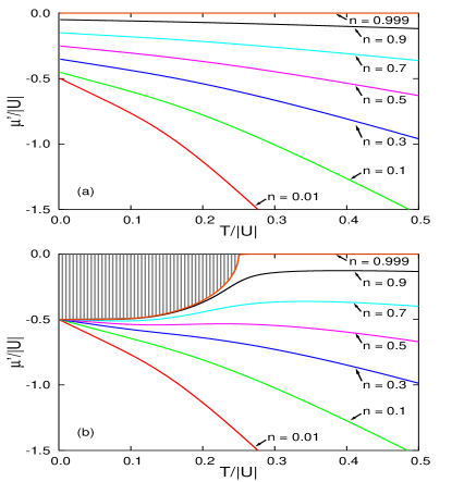
Figure 1: (a) Exact solutions and (b) $(G_{0}G_{0})G_{0}$ results for $\mu^{\prime}$ vs. temperature for different densities. In (b) the shaded region is the so-called Thouless region. Note that it is absent in the exact solution.

The non-self-consistent (NSC) approximation was first examined in two dimensions for the AHM in Refs. schmitt-rink89 ; serene89 . Fig. (1b) shows the results in the atomic limit. Comparison with Fig. (1a) shows that this approximation is poor; indeed the same conclusion occurs in two dimensions beach01 . A ‘Thouless region’ in the $\mu^{\prime}-T$ plane occurs; this is where an instability would occur if $\mu^{\prime}$ was held fixed while the temperature is lowered; it is indicated in Fig. (1b) by the shaded region. The more physical procedure is to keep the electron density fixed. Then $\mu^{\prime}$ adjusts so that a finite temperature transition is avoided. As in higher dimensions, the electrons form bound states, the Fermi sea is depleted, and a finite temperature transition is avoided for the wrong reason, as inspection of Fig. (1a) shows.

We have examined all the possible variations for Eqs.(7, 8) at low electron densities. The results for $\mu^{\prime}$ vs. $T$ at a low electron density are shown in Fig. (2a). In addition we have also computed the result for the Vilk-Tremblay kyung01 theory. At very low electron densities all approximations work reasonably well. At low (but not too low) electron densities, two emerge as particularly accurate, the $(GG_{0})G_{0}$ T-matrix theory, and the Vilk-Tremblay theory. We use a nomenclature for the T-matrix theory to correspond to $(G_{a}G_{b})G_{c}$, where the $a$, $b$, and $c$ refer to the labels in Eqs.(7, 8).

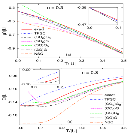
Figure 2: A comparison of different approximations at n = 0.3 using (a) $\mu^{\prime}$, and (b) energy. Note that the VT result (first iteration only) and the $(GG_{0})G_{0}$ T-matrix approximation are the most accurate; they both become exact as $T\rightarrow 0$. The second iteration of the VT result (not shown) is poorer than the first. The insets focus on the TPSC and $(GG_{0})G_{0}$ results at low temperatures; note in (b) how well the $(GG_{0})G_{0}$ curve approaches the exact result over an extended temperature range.

Clearly, the Vilk-Tremblay result is most accurate. However, particularly at low temperatures, it is evident that the $(GG_{0})G_{0}$ T-matrix approximation is also quite accurate. In fact, at lower electron densities (not shown) the $(GG_{0})G_{0}$ result becomes more accurate than the VT result, and these two remain the front-runners for all electron densities. Interestingly, both the VT and the $(GG_{0})G_{0}$ results appear to become exact at low temperatures. Indeed, in the $(GG_{0})G_{0}$ formulation the ansatz

$$\Sigma(i\omega_{m})={\Delta^{2}\over i\omega_{m}-\mu^{\prime}}$$ (9)

emerges if one considers only the term in Eq. (7) with ${\ell}=0$. Then $\Delta^{2}=T|U|^{2}\chi_{0}(0)/(1-|U|\chi_{0}(0))$. Insertion of this self energy into the one electron Green function allows one to evaluate the bare susceptibility in Eq. (8) at zero frequency. Earlier work beach01 indicated that any degree of self-consistency in the ’bare’ susceptibility drives the superconducting transition (signalled by $1=|U|\chi_{0}(0)$) to zero temperature. Adopting this requirement in this case gives the parameter $\Delta^{2}$ in terms of $|U|$ and $\mu^{\prime}$. The number equation, $n={2\over\beta}\sum_{m}G(i\omega_{m})\exp{(i\omega_{m}0^{+})}$ provides a second relation between $\Delta^{2}$ and $\mu^{\prime}$; with these two equations all the zero temperature properties can be obtained analytically, and, remarkably, they agree with the exact solution. Thus, the suppression of the Thouless instability to zero temperature is a feature in common with higher dimensional solutions. For the VT theory, these results are for the first iteration kyung01 . If one presses further with the second iteration, the results deteriorate, consistent with the observation of these authors allen04 .

We can press further these comparisons, and in particular probe two-particle correlations. An easy way to do this is by examining the energy per lattice site $E$, which normally would be simply proportional to the double occupancy in the atomic limit. However, because of the special form of the Hamiltonian, Eq. (1), the precise relation is

$$E=-|U|<n_{\uparrow}n_{\downarrow}>+|U|\bigl{(}{n\over 2}\bigr{)}^{2}.$$ (10)

We use the exact relation

$$E={1\over\beta}\sum_{m}\Sigma(i\omega_{m})G(i\omega_{m})\exp{(i\omega_{m}0^{+})},$$ (11)

to obtain the energy at any temperature, in the T-matrix theories. Fig. (2b) shows the energy determined within the various approximation schemes along with the exact and the VT result, for $n=0.3$. Once again the VT and $(GG_{0})G_{0}$ results are exact at zero temperature. However, the VT result deviates immediately for $T>0$, while the $(GG_{0})G_{0}$ result follows closely over some temperature range. That this latter result is true follows also from the analytical work described above.

This agreement at $T=0$ (note that neither approximation is particularly accurate at intermediate temperatures) raises the question of the origin of the effective potential, $|U_{pp}|$, in the VT theory. Within a conserving approxmiation, a frequency-independent irreducible vertex, $|U_{pp}|$, is accompanied by single electron propagators that include a simple Hartree-like renormalization kyung01 . The $(GG_{0})G_{0}$ T-matrix approach, however, suggests that the origin of an effective interaction is from the (partial) renormalization of the single electron propagator. That is, we can construct a theory that appears similar to the VT theory, i.e. with unrenormalized propagators everywhere in Eqs.(7,8), but with an effective interaction vertex. Eq.(7) suggests this will be accomplished by

$$|U|\chi_{0}(i\nu_{n})\equiv|U_{eff}|\chi_{00}(i\nu_{n}),$$ (12)

where $\chi_{00}(i\nu_{n})={1\over\beta}\sum_{m}G_{0}(i\omega_{m})G_{0}(-i\omega_{m}+i\nu_{n})$. Note that this requires $|U_{eff}|$ to depend on Matsubara frequency, but, in the spirit of VT (and many Parquet-like treatments of higher order corrections bickers04 ), we will use Eq. (12) at zero Matsubara frequency to define an effective potential. Comparisons with $|U_{pp}|$ as obtained in the VT formalism show quantitative discrepancies, particularly as the temperature approaches zero. Thus, the two theories differ more substantively than Eq. (12) would suggest.

To probe further the analytical structure of the various approximations, we examine the spectral function ($A(\omega)\equiv-{\rm Im}G(\omega+i\delta)/\pi$). As already noted, the $(GG_{0})G_{0}$ reproduces the exact result at zero temperature. This is shown in Fig. 3, where the spectral function for the $(GG_{0})G_{0}$ has been obtained through Padé approximants. The agreement with the exact result at low temperatures is remarkable. On the other hand, the VT result in the first iteration gives a single pole, which is clearly inaccurate. The result obtained from the second iteration does contain two poles. However, as shown, it is fairly inaccurate. Thus, even though both the VT theory and the $(GG_{0})G_{0}$ T-matrix approximation give exact results for the chemical potential and the energy at low temperatures, only the latter fully reproduces the exact result as a function of frequency. Inspection of Fig. 2 shows that ‘improving’ the degree of self-consistency deteriorates the agreement. This would mean that at low temperatures some cancellation occurs between the fully self-consistent T-matrix diagrams ($(GG)G$ theory) and the omitted vertex corrections. This possibility remains to be shown, however.

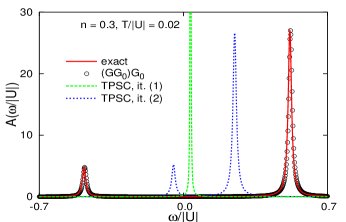
Figure 3: The spectral function for the $(GG_{0})G_{0}$ T-matrix approximation (symbols), compared with the exact result (solid curve). The remarkable agreement shows that only partial self-consistency is a requirement to reproduce the exact result. The VT result (both first and second iterations) are poorer in comparison. We have used a small artificial broadening, $\delta=0.01|U|$ to plot these results.

In summary we have critically examined various approximations for the attractive Hubbard model in the dilute and strong coupling limit. We have used a variety of self-consistent T-matrix approaches along with the two-particle self-consistent (VT) phenomenology. We found that minimal self-consistency (the $(GG_{0})G_{0}$ theory promoted in particular in Ref. janko97 ) and the VT calculation both reproduced the exact result best, particularly at low temperatures, where both become exact. Surprisingly, ‘improving’ the degree of self-consistency within a T-matrix approach leads to less accurate results vilk97_comment . Two particle correlations (summarized in the total energy in this work) are faithfully reproduced by the $(GG_{0})G_{0}$ calculation for a range of low temperatures, and, finally, the one electron spectral function is remarkably accurate, even at nonzero temperature. These results suggest that, at least for low electron densities, this T-matrix formulation is useful for higher dimension calculations. It would also be interesting to see how the various vertex corrections provide partial cancellation to the omitted self-consistent contributions.

This work was supported in part by the Natural Sciences and Engineering Research Council of Canada (NSERC), by ICORE (Alberta), and by the Canadian Institute for Advanced Research (CIAR).

References

- (1) P.W. Anderson, Physics Today, Feb. 2000, p. 11.
- (2) J. Bardeen, L.N. Cooper and J.R. Schrieffer, Phys. Rev. 106, 162 (1957); Phys. Rev. 108, 1175 (1957).
- (3) L.P. Gor’kov, Soviet Physics JETP-USSR 7, 505 (1958).
- (4) G.M. Eliashberg, Zh. Eksperim. i Teor. Fiz. 38 966 (1960) [Soviet Phys. JETP 11 696 (1960)].
- (5) D.J. Thouless, Ann. Phys. 10, 553 (1960).
- (6) L.P. Kadanoff and P.C. Martin, Phys. Rev 124, 670 (1961).
- (7) D. M. Eagles, Phys. Rev. 186, 456 (1969).
-
(8)
A.J. Leggett, J. de Physique, C7, 41, 19 (1980);
A.J. Leggett, in Modern Trends in the Theory of Condensed Matter, edited by S. Pekalski and J. Przystawa (Springer, Berlin, 1980) p. 13. - (9) P. Nozières and S. Schmitt-Rink, J. Low Temp. Phys. 59, 195 (1985).
- (10) B. Janko, J. Maly, and K. Levin, Phys. Rev. B 56, 11407 (1997); I. Kosztin, Q. Chen, B. Janko, and K. Levin, Phys. Rev. B 58, 5936 (1998). See also Q. Chen, K. Levin, and I. Kosztin, Phys. Rev. B 63, 184519 (2001), and references therein.
- (11) R.J. Gooding, F. Marsiglio, S. Verga, and K.S.D. Beach, J. Low Temp. Phys. 136, 191 (2004). See also cond-mat/0401609.
- (12) J. Vilk and A.-M.S. Tremblay, J. de Physique I (France) 7, 1309 (1997).
- (13) S. Allen and A.-M.S. Tremblay, Phys. Rev. B 64, 075115 (2001).
- (14) B. Kyung, S. Allen, and A.-M.S. Tremblay, Phys. Rev. B64, 075116 (2001).
- (15) P. Pieri an G.C. Strinati, Phys. Rev. B 61, 15370 (2000).
- (16) K. Kanamori, Prog. Theor. Phys. 30, 275 (1963).
- (17) V. Zlatić, B. Horvatić, B. Dolicki, S. Grabowski, P. Entel, and K.-D. Schotte, Phys. Rev. B63, 035104 (2000).
- (18) R. Micnas, M. H. Pedersen, S. Schafroth, T. Schneider, J. J. Rodríguez-Núñez and H. Beck, Phys. Rev. B52, 16223 (1995).
- (19) K.S.D. Beach, R.J. Gooding, and F. Marsiglio, Phys. Lett. A 282, 319 (2001).
- (20) S. Schmitt-Rink, C. Varma, and A.E. Ruckenstein, Phys. Rev. Lett. 63, 445 (1989).
- (21) J. Serene, Phys. Rev. B 40, 10873 (1989).
- (22) S. Allen, A.-M.S. Tremblay, and Y.M. Vilk, in Theoretical Methods for Strongly Correlated Electrons, edited by D. Sénéchal, A.-M. Tremblay, and C. Bourbonnais, Springer, 2004, p. 341.
- (23) N.E. Bickers, in Ref. allen04 , p. 235.
- (24) Although arguments for why this might be expected were advanced in Ref. vilk97 .