Spin glasses in the limit of an infinite number of spin components.

Abstract

We consider the spin glass model in which the number of spin components, $m$, is infinite. In the formulation of the problem appropriate for numerical calculations proposed by several authors, we show that the order parameter defined by the long-distance limit of the correlation functions is actually zero and there is only “quasi long range order” below the transition temperature. We also show that the spin glass transition temperature is zero in three dimensions.

I Introduction

It is of interest to study a spin glass model in which the number of components of spin components $m$ is infinite, because it provides some simplifications compared with Ising ($m=1$) or Heisenberg ($m=3$) models. For example, in mean field theory (i.e. for the infinite range model) there is no “replica symmetry breaking” de Almeida et al. (1978) so the ordered state is characterized by a single order parameter $q$, rather than by an infinite number of order parameters (encapsulated in a function $q(x)$) which are needed Parisi (1980) for finite-$m$.

There has recently been renewed interest  Hastings (2000); Aspelmeier and Moore (2004) in the $m=\infty$ model, and the interesting result emerged from these studies that the effective number of spin components depends on the system size $N$ and is only really infinite in the thermodynamic limit. One motivation for the present study is to investigate some consequences of this result.

Further motivation for our present study comes from earlier work by two of us Lee and Young (2003) which argued that an isotropic vector spin glass ($m\geq 2$), as well as an Ising spin glass, has a finite spin glass transition temperature $T_{SG}$ in three dimensions. The results of Ref. [Lee and Young, 2003] also indicate that $T_{SG}$ is very low compared with the mean field transition temperature, $T_{SG}^{MF}$, and decreases with increasing $m$, see Table 1. The results in Table 1 suggest that $T_{SG}/T_{SG}^{MF}$ may be zero in the $m=\infty$ limit in three dimensions, and we investigate this possibility here.

$m$	model	$T_{SG}^{MF}$	$T_{SG}$	$T_{SG}/T_{SG}^{MF}$
1	Ising	$2.45$	0.97 [Marinari et al., 1998; Young and Katzgraber, 2004]	0.40
2	XY	$1.22$	0.34 [Lee and Young, 2003]	0.28
3	Heisenberg	$0.82$	0.16 [Lee and Young, 2003]	0.20

Table 1: Estimates of the spin glass transition temperature, relative to the mean field value, $T_{SG}^{MF}=\sqrt{z}/m$, see Eq. (2), for different values of $m$ for the three-dimensional simple cubic lattice ($z=6$). The factor of $1/m$ in $T_{SG}^{MF}$, appears because the spins were normalized to unity in Refs. [Lee and Young, 2003; Marinari et al., 1998; Young and Katzgraber, 2004], rather than to $m^{1/2}$ as here. For the model used in this paper, $T_{SG}^{MF}$ is finite for $M\to\infty$.

In this paper, we study the $m=\infty$ SG model, both the infinite range version and the short-range model in three and two dimensions. We find that we need to carefully specify the order in which the limits $m\to\infty$ and the thermodynamic limit $N\to\infty$ are taken. In Ref. de Almeida et al., 1978, the $N\to\infty$ limit is taken first (since a saddlepoint calculation is performed) and the $m\to\infty$ limit is taken at the end. However, in the formulation of the $m=\infty$ problem which has been proposed for numerical implementation in finite dimensions Bray and Moore (1982); Morris et al. (1986); Hastings (2000); Aspelmeier and Moore (2004) and which we use here, the limit $m\to\infty$ is taken first for a lattice of finite size. In the latter case, we find that for $T<T_{SG}$ the spin glass correlations decay with a power of the distance $r$ and tend to zero for $r\to\infty$, so the order parameter, defined in terms of the long-distance limit of the correlation function, is actually zero. Nonetheless, there can still be a transition at $T_{SG}$ separating a high temperature phase where the correlations decay exponentially, from the the low temperature phase where they decay with a power law. By contrast, if one takes $N\to\infty$ first with $m$ finite, the power law decay eventually changes to a constant at large $r$ and so a non-zero spin glass order parameter can be defined, as in Ref. de Almeida et al., 1978.

We give phenomenological arguments for these conclusions and back them up (for the case where $m\to\infty$ is taken first) by numerical results at zero temperature. We also find, from numerical results at finite temperature, that $T_{SG}/T_{SG}^{MF}=0$ in three dimensions for $m=\infty$, consistent with the trend of the results in Table 1.

In Sec. II we discuss the model and the methods used to study it numerically. In Sec. III we describe our results at $T=0$ for both short-range and the infinite-range model, while in Sec. IV we describe finite temperature results for short-range models. Our conclusions are summarized in Sec. V.

II Model and method

We take the Edwards-Anderson Edwards and Anderson (1975) Hamiltonian

$${\cal H}=\sum_{\langle i,j\rangle}J_{ij}\mathbf{S}_{i}\cdot\mathbf{S}_{j}\,,$$ (1)

where the spins $\mathbf{S}_{i}$ ($i=1,\cdots,N$) are classical vectors with $m$ components and normalized to length $m^{1/2}$, i.e. $\mathbf{S}_{i}^{2}=m$. As we shall see, this normalization is necessary to get a finite transition temperature in the mean field limit. The $J_{ij}$ are independent random variables with a Gaussian distribution with zero mean. We consider both the infinite range model and short-range models with nearest-neighbor interactions in two and three dimensions. For the infinite range model, the standard deviation is taken to be $1/\sqrt{N-1}$ while for the short-range models the standard deviation is set to be unity. According to the mean field approximation, the spin glass transition temperature is

$$T_{SG}^{MF}={\langle\mathbf{S}_{i}^{2}\rangle\over m}\left[\sum_{j}J_{ij}^{2}\right]_{\mathrm{av}}^{1/2}\,,$$ (2)

where $[\cdots]_{\mathrm{av}}$ indicates an average over the disorder. Hence, for the infinite range model, (where mean field theory is exact) Eq. (2) gives $T_{SG}=T_{SG}^{MF}=1$, while for the short-range case it gives $T_{SG}^{MF}=\sqrt{z}$, where $z$ is the number of nearest neighbors (4 for the square lattice and 6 for the simple cubic lattice).

As shown in other work Bray and Moore (1982); Morris et al. (1986); Hastings (2000); Aspelmeier and Moore (2004), the problem can be simplified for $m=\infty$. The spin-spin correlation function,

$$C_{ij}\equiv{1\over m}\langle\mathbf{S}_{i}\cdot\mathbf{S}_{j}\rangle,$$ (3)

is given by

$$T^{-1}C_{ij} = \left(A^{-1}\right)_{ij},\qquad\mbox{where}$$ (4)

$$A_{ij} = H_{i}\delta_{ij}-J_{ij},$$ (5)

and the $H_{i}$ have to be determined self consistently to enforce (on average) the length constraint on the spins,

$$C_{ii}=1\,.$$ (6)

Angular brackets, $\langle\cdots\rangle$, refer to a thermal average for a given set of disorder. Eq. (6) with $i=1,\cdots,N$ represents $N$ equations which have to be solved for the $N$ unknowns $H_{i}$. In Sec. IV we will solve these equations numerically for a range of sizes at finite temperature. We emphasize that in Eqs. (3)–(6) the limit $m\to\infty$ has been taken with $N$ finite. This is the opposite order of limits from that in the analytical work of Ref. de Almeida et al., 1978 where $N\to\infty$ was taken before $m\to\infty$. As we shall see, the results from the two orders of limits are different.

Figure 1: A plot of the effective number of spin components as a function of system size $N$. For small $N$, $m_{0}\sim N^{\mu}$, but once $m_{0}$ hits the actual number of spin components $m$, it sticks at $m$ as $N$ is further increased.

Eqs. (3)–(6) are not well defined at $T=0$. However, Aspelmeier and Moore Aspelmeier and Moore (2004) pointed out that one can solve the $m=\infty$ problem directly at $T=0$, using the following method. At zero temperature there are no thermal fluctuations so each spin lies parallel to its local field, i.e.

$$\textbf{S}_{i}=H_{i}^{-1}\sum_{j}J_{ij}\textbf{S}_{j}\,,$$ (7)

where $m^{1/2}H_{i}$ is the magnitude of the local field on site $i$. Remarkably, it was shown by Hastings Hastings (2000) that these local fields are precisely the zero temperature limit of the $H_{i}$ in Eq. (5). Hastings Hastings (2000) also showed that the number of independent spin components which are non-zero in the ground state, which we call $m_{0}$, cannot be arbitrarily large, but satisfies the bound

$$m_{0}<\sqrt{2N}\,.$$ (8)

This means that one can always perform a global rotation of the spins such that only $m_{0}$ components have a non-zero expectation value and the remaining $m-m_{0}$ components vanish. Thus one can think of $m_{0}$ as the effective number of spin components. If $m$ is finite, then, at some value of $N$, $m_{0}$ would equal the actual number of spin components $m$. At this point, all spin components are used so $m_{0}$ “sticks” at the value $m$ as $N$ is further increased, see Fig. 1.

More generally we can write Eq. (8) as

$$m_{0}\sim N^{\mu},\quad(m_{0}<m)$$ (9)

and the bound in Eq. (8) gives $\mu\leq 1/2$. Later, we will determine $\mu$ numerically for several models. For Eqs. (3)–(6) to be valid we need $m>m_{0}$ which corresponds to the curved part of the line in Fig. 1. As discussed above, this corresponds to taking the limit $m\to\infty$ first, followed by the limit $N\to\infty$. Since $m_{0}$ increases with $N$ one needs larger values of $m$ for larger lattice sizes. This will be important in what follows.

We therefore see that we can numerically solve the $m=\infty$ problem at $T=0$ on a finite lattice by taking a number of spin components which is finite but greater than $m_{0}$, and solving Eqs. (7). To do this we cycle through the lattice, and at site $i$, say, we calculate $H_{i}$ from

$$H_{i}={1\over m^{1/2}}\left|\sum_{j}J_{ij}\mathbf{S}_{j}\right|\,.$$ (10)

We then set $\mathbf{S}_{i}$ to the value given by Eq. (7) so it lies parallel to its instantaneous local field. This is repeated for each site $i$, and then the whole procedure iterated iterated to convergence. Although spin glasses with finite-$m$ have many solutions of Eqs. (7), it turns out that for $m=\infty$ (in practice this means $m>m_{0}$) there is a unique stable solution Bray and Moore (1981), so the numerical solution of Eqs. (7) is straightforward. We will discuss our numerical results at $T=0$ using Eqs. (7) in Sec. III, and here we simply note that we do indeed find a unique solution of these equations.

Next we consider the order parameter in spin glasses for $m=\infty$. In the absence of a symmetry breaking field, one defines the long range order parameter, $q$, by the behavior of the spin-spin correlation function $[C_{ij}^{2}]_{\mathrm{av}}$ at large distances, i.e.

$$q^{2}=\lim_{R_{ij}\to\infty}[C_{ij}^{2}]_{\mathrm{av}}\,\qquad\mbox{(short\ range),}$$ (11)

where $R_{ij}=|\mathbf{R}_{i}-\mathbf{R}_{j}|$. For the infinite-range model, any distinct pair of sites will do, and so

$$q^{2}=[C_{ij}^{2}]_{\mathrm{av}}\ (i\neq j)\qquad\mbox{(infinite\ range).}$$ (12)

We now give phenomenological arguments, which will be supported by numerical data in Sec. III, that $q$ obtained from Eqs. (11) and (12), in which $C_{ij}$ is determined by Eqs. (3)–(6), is actually zero for $m=\infty$, and that, at best, spin correlations have only “quasi-long range order”. For the short range case, this means that $[C_{ij}^{2}]_{\mathrm{av}}$ decays with a power of the distance $R_{ij}$, while for the infinite range model the correlation function in Eq. (12) tends to zero with a power of $N$.

To see why this is the case, we take $T=0$ and consider first the infinite-range model. For a given $N$, the spins “splay out” in $m_{0}\sim N^{\mu}$ directions. We expect the spins to point, on average, roughly equally in all directions in this $m_{0}$-dimensional space. Now $C_{ij}$ in Eq. (3) is equal to $\cos\theta_{ij}$ where $\theta_{ij}$ is the angle between $\mathbf{S}_{i}$ and $\mathbf{S}_{j}$. We take the square and average equally over all directions. To do the average, take a coordinate system with the polar axis along $\mathbf{S}_{i}$, so $\theta_{ij}=\theta_{j}$ the polar angle of $\mathbf{S}_{j}$. Then we have

$$q^{2} = [C_{ij}^{2}]_{\mathrm{av}}=\langle\cos^{2}\theta_{j}\rangle$$ (13)

$$= {1\over\mathbf{S}^{2}}\langle S_{z}^{2}\rangle\sim{1\over m_{0}}{\sum_{\alpha=1}^{m_{0}}\langle S_{\alpha}^{2}\rangle\over\mathbf{S}^{2}}={1\over m_{0}}\sim N^{-\mu}\,,$$

where we used the result that the average is roughly the same for all the $m_{0}$ spin components. Since $\mu$ will turn out to be non-zero it follows that the order parameter tends to zero with a power of the size of the system. The same will be true at temperatures $T<T_{SG}$, while above $T_{SG}$ the order parameter as defined here will vanish faster, as $1/N$.

How can we reconcile this vanishing order parameter with earlier results de Almeida et al. (1978) that the order parameter is non zero below $T_{SG}=1$, and in particular is unity at $T=0$. The difference comes in part because $q^{2}$ in Ref. [de Almeida et al., 1978], which we call $q^{2}_{\rm AJKT}$, is $m$ times our $q^{2}$, and so

$$q^{2}_{\rm AJKT}=mq^{2}\sim{m\over m_{0}},\quad(T=0).$$ (14)

The other difference is that Ref. [de Almeida et al., 1978] performs the limit $N\to\infty$ first, which corresponds to being on the horizontal part of the line in Fig. 1, so $m_{0}=m$. From Eq. (14) we then get $q^{2}_{\rm AJKT}=\text{const.}$ at $T=0$ in agreement with Ref. [de Almeida et al., 1978].

Going back to the calculation of $C_{ij}$, if one sums $[C_{ij}^{2}]_{\mathrm{av}}$ for the infinite range model over all pairs of sites we find that the spin glass susceptibility ${\chi_{\rm SG}}$ at $T=0$ is given by

$${\chi_{\rm SG}}={1\over N}\sum_{i,j}[C_{ij}^{2}]_{\mathrm{av}}=1+(N-1)q^{2}\simeq Nq^{2}\sim N^{1-\mu}\,.$$ (15)

Turning now to the short-range case, we expect that ${\chi_{\rm SG}}\sim N^{1-\mu}$ will still be true, which implies that correlations decay with a power of distance. Assuming that $[C_{ij}^{2}]_{\mathrm{av}}\sim 1/R_{ij}^{y}$ for some exponent $y$, then integrating over all $\mathbf{r}$ up to $r=L$ (where $N=L^{d}$) and requiring that the result goes as $N^{1-\mu}$, gives $y=d\,\mu$, i.e.

$$[C_{ij}^{2}]_{\mathrm{av}}\sim{1\over R_{ij}^{d\,\mu}}\,.$$ (16)

Such power law decay is often called “quasi long range order”. We expect that Eq. (16) will be true quite generally at $T=0$ and everywhere below $T_{SG}$ if $T_{SG}>0$. Note that this implies that $q=0$ according to Eq. (11). Above $T_{SG}$, $[C_{ij}^{2}]_{\mathrm{av}}$ will decay to zero exponentially with distance.

If $m$ is large but finite, then $[C_{ij}^{2}]_{\mathrm{av}}$ will saturate when $R_{ij}$ is sufficiently large that all the spin components are used. This happens when $[C_{ij}^{2}]_{\mathrm{av}}\sim 1/m$, i.e. for $R_{ij}\gtrsim m^{1/d\,\mu}$. In this case, $q^{2}_{\rm AJKT}=mq^{2}$ will be finite according to Eq. (11).

$N$	$N_{\rm samp}$
32	$1000$
64	$1000$
128	$1000$
256	$1000$
512	$1000$
1024	$777$
2048	$302$

Table 2: Number of samples used in the $T=0$ studies of the infinite-range model.

Figure 2: The average number of non-zero spin components in the ground state, $m_{0}$, as a function of $N$ for the infinite-range model. We see that $m_{0}$ increases like $N^{\mu}$ with $\mu$ close to $2/5$ as expected.

Figure 3: The square of the order parameter at $T=0$ for infinite range model. As expected it decreases like $N^{-\mu}$ with $\mu=2/5$.

In Secs. III.1 and III.2 we will provide numerical support for Eq. (15) for the infinite-range and short-range cases respectively.

III Results at zero temperature

III.1 Infinite Range Model

We consider a range of lattice sizes up to $N=2048$ and for each size the number of samples is shown in Table 2.

The average number of non-zero spin components in the ground state is given by Eq. (9), for which it has been shown thatAspelmeier and Moore (2004); Hastings (2000)

$$\mu=2/5\,,\qquad\mbox{(infinite\ range.)}$$ (17)

exactly. This result has been confirmed numerically Aspelmeier and Moore (2004). Our results for $\mu$ are shown in Fig. 2 and indeed give $\mu$ close to 2/5. The small deviation is presumably due to corrections to scaling.

We also calculated $q^{2}$ at $T=0$ from Eq. (12). In Eq. (3) the thermal average, $\langle\cdots\rangle$, is unnecessary, and the spin directions are determined by solving Eqs.  (7) and (10). The results for are shown in Fig. 3, showing that it vanishes with exponent $-\mu$ as a function of $N$, as expected from Eq. (13).

Figure 4: The average number of non-zero spin components in the ground state, $m_{0}$, as a function of $N$ for the short-range model in $d=3$. We see that $m_{0}$ increases like $N^{\mu}$ with $\mu\simeq 0.33$.

	$T=0$		$T>0$
$L$	$N_{\rm samp}\ (m_{0})$	$N_{\rm samp}\ ({\chi_{\rm SG}})$	$N_{\rm samp}$
3	$1000$	–	–
4	$1000$	$1000$	$100$
6	$1000$	$1000$	$100$
8	$1000$	$1000$	$100$
10	$1000$	–	–
12	$1105$	$1105$	$100$
16	$785$	$785$	–
24	–	$500$	–

Table 3: Number of samples used in the calculations for the short-range model in three-dimensions.

Figure 5: The spin glass susceptibility for the short-range model in $d=3$ for different system sizes. As expected it varies as $N^{1-\mu}$, where $\mu\simeq 0.33$ was also found in Fig. 4.

	$T=0$		$T>0$
$L$	$N_{\rm samp}\ (m_{0})$	$N_{\rm samp}\ ({\chi_{\rm SG}})$	$N_{\rm samp}$
4	$1000$	$1000$	$1000$
6	$1000$	$1000$	$1000$
8	$1000$	$1000$	$1000$
10	$1000$	–	–
12	$1000$	$1000$	$1000$
14	$1000$	–	–
16	$1000$	$1000$	$1000$
18	$1000$	–	–
20	$1000$	–	–
22	$1000$	–	–
24	–	$1000$	$500$
28	$1000$	–	–
32	$1000$	$1000$	$309$
48	–	$472$	$136$
64	$1016$	$1016$	–

Table 4: Number of samples used in the calculations for the short-range model in two-dimensions.

Figure 6: The average number of non-zero spin components in the ground state, $m_{0}$, as a function of $N$ for the short-range model in $d=2$. We see that $m_{0}$ increases like $N^{\mu}$ with $\mu\simeq 0.29$.

Figure 7: The spin glass susceptibility for the short-range model in $d=2$ for different system sizes. As expected it varies as $N^{1-\mu}$, where $\mu\simeq 0.29$ was also found in Fig. 6.

III.2 Short Range models

First of all we describe our results for three dimensions. The number of samples is shown in Table 3.

Our results for $\mu$ are shown in Fig. 4, indicating that $\mu\simeq 0.33$, definitely different from the infinite range result of $2/5$. The results for ${\chi_{\rm SG}}$ as a function of $N$ are shown in Fig. 5. We see that ${\chi_{\rm SG}}$ grows with an exponent $1-\mu$ with the same value of $\mu$ as in Fig. 4. We therefore find that $d\,\mu\simeq 1.0$, and so, from Eq. (16), the spin glass correlations decay as

$$[C_{ij}]^{2}_{\mathrm{av}}\sim{1\over R_{ij}},\qquad(d=3,\ T=0)\,.$$ (18)

(It is of course possible that power of $R_{ij}$ may not be exactly $-1$.)

Next we describe our results for two dimensions. The number of samples used is shown in Table 4. Our results for $\mu$ are shown in Fig. 6, and give $\mu\simeq 0.29$. The data for ${\chi_{\rm SG}}$ is shown in Fig. 7. We see that ${\chi_{\rm SG}}$ increases as $N^{1-\mu}$ with the same $\mu$ as determined from Fig. 6. We therefore find that $d\,\mu\simeq 0.58$, and so, from Eq. (16), the spin glass correlations decay as

$$[C_{ij}]^{2}_{\mathrm{av}}\sim{1\over R_{ij}^{0.58}},\qquad(d=2,\ T=0)\,.$$ (19)

IV Results for short range models at finite temperature

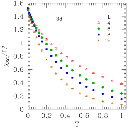
Figure 8: The spin glass susceptibility as a function of temperature in three dimensions. The vertical axis has been divided by $L^{d(1-\mu)}$, in which we took $\mu=1/3$ in order to collapse the data at $T=0$ according to the data in Figs. 4 and 5.

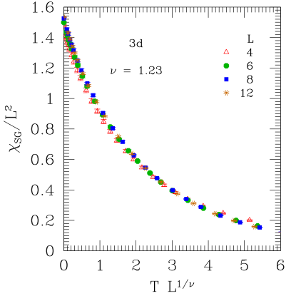
Figure 9: A scaling plot of the spin glass susceptibility in Fig. 8 assuming a zero temperature transition.

We have determined finite temperature properties by solving Eqs. (4)–(6) self-consistently using the Newton-Raphson method. We start at high temperature, $T=T_{1}$ say, and take our initial guess to be $H_{i}=1/\beta$ which is the solution obtained perturbatively to first order in $1/T$. We then solve the equations at successively lower temperatures, $T_{1}>T_{2}>T_{3}>T_{4}\cdots$, and obtain the initial guess for the $H_{i}$ at temperature $T_{i+1}$ by integrating the equations Aspelmeier and Moore (2004)

$${dH_{i}\over d\beta}=-\sum_{j}\left(B^{-1}\right)_{ij}\,,$$ (20)

in which

$$B_{ij}=(\beta C_{ij})^{2}\,,$$ (21)

from $\beta_{i}$ to $\beta_{i+1}$ ($\beta=1/T$).

Results for ${\chi_{\rm SG}}$ in $d=3$ are shown in Fig. 8, in which we scaled the vertical axis by $L^{d(1-\mu})\ (=L^{2})$ so the data collapses at $T=0$. If we assume a zero temperature transition, the data should fit the finite-size scaling form

$${\chi_{\rm SG}}=L^{d(1-\mu)}X\left(L^{1/\nu}T\right)\,.$$ (22)

where $X(x)\to\text{const.}$ for $x\to 0$, and the power law prefactor in front of the scaling function $X(x)$ then gets the $T=0$ limit correct. Figure  9 shows an appropriate scaling plot with $\nu=1.23$. Apart from the smallest size, $L=4$, the data clearly collapses well. By considering different values of $\nu$ we estimate

$$\nu=1.23\pm 0.13\qquad(d=3)\,.$$ (23)

This result can be compared with that of Morris et al. Morris et al. (1986) who quote $\nu=1.01\pm 0.02$. Since our results cover a larger range of sizes and have better statistics, we feel that the error bars of Morris et al. are too optimistic. Assuming this, our result is consistent with theirs.

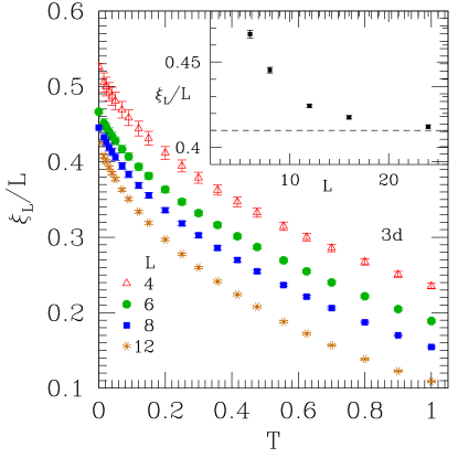
Figure 10: The main figure is a plot of $\xi_{L}/L$ against $T$ in three dimensions. The inset shows $\xi_{L}/L$ at $T=0$ as a function of $L$. The dashed line is a guide to the eye.

We should, however, also test to see if the data can be fitted with a finite value for $T_{SG}$. To do this, it is convenient to analyze the correlation length of the finite system, $\xi_{L}$, and plot the dimensionless ratio $\xi_{L}/L$ which has the expected scaling form Ballesteros et al. (2000); Lee and Young (2003)

$${\xi_{L}\over L}=F\left(L^{1/\nu}(T-T_{SG})\right)\,$$ (24)

without any unknown power of $L$ multiplying the scaling function $F$. Hence the data for different sizes should intersect at $T_{SG}$ and also splay out below $T_{SG}$. To determine $\xi_{L}$ we Fourier transform $[C_{ij}^{2}]_{\mathrm{av}}$ to get ${\chi_{\rm SG}}({\bf k})$ and then use Ballesteros et al. (2000); Lee and Young (2003)

$$\xi_{L}={1\over 2\sin(k_{\rm min}/2)}\left({{\chi_{\rm SG}}(0)\over{\chi_{\rm SG}}({\bf k}_{\rm min})}-1\right)^{1/2}\,,$$ (25)

where ${\bf k}_{\rm min}=(2\pi/L)(1,0,0)$ is the smallest non-zero wavevector on the lattice.

The results are shown in the main part of Fig. 10. The data don’t intersect at any temperature, but seem to be approaching an intersection at $T=0$ for the larger sizes. To test out this possibility, we have computed the correlation length directly at $T=0$, from the solution of Eqs. (7) and (10), where we can study larger sizes than in the finite-$T$ formulation of Eqs. (3)–(6). The data is shown in the inset to Fig. 10. It indicates, fairly convincingly, that $\xi_{L}/L$ approaches a constant for $L\to\infty$ at $T=0$, and hence that there is a transition at $T=0$.

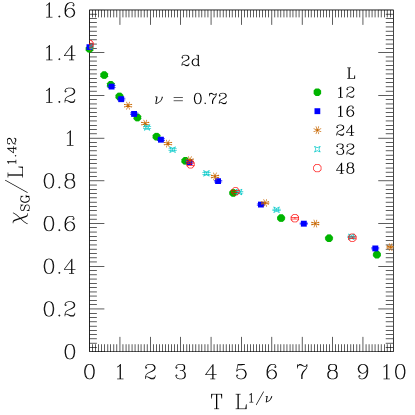
Figure 11: A scaling plot of the data for ${\chi_{\rm SG}}$ in two dimensions, assuming a zero temperature transition. In the vertical axis, ${\chi_{\rm SG}}$ is divided by $L^{d(1-\mu)}\simeq L^{1.42}$ so that the data collapses at $T=0$.

In $d=2$ it is well established that $T_{SG}=0$ even for the Ising case. A scaling plot for ${\chi_{\rm SG}}$ for $m=\infty$ in $d=2$, corresponding to Eq. (22), is shown in Fig. 11 with $\nu=0.72$, which gives the best data collapse for larger sizes, and $d(1-\mu)=1.42$ which is obtained from the $T=0$ results in Sec. III. Again the data scales well. Overall we estimate

$$\nu=0.72\pm 0.05\qquad(d=2,\quad\text{from }{\chi_{\rm SG}})\,.$$ (26)

This is consistent with the results in Morris et al. Morris et al. (1986) who quote $\nu=0.65\pm 0.02$.

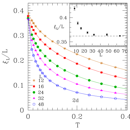
Figure 12: Data for $\xi_{L}/L$ as a function of $T$ in two dimensions. Clearly the data for larger sizes is merging at $T=0$ indicating a transition at $T_{SG}=0$. The inset shows data for $\xi_{L}/L$ at $T=0$ confirming that the data becomes independent of size at $T=0$. The dashed line is a guide to the eye.

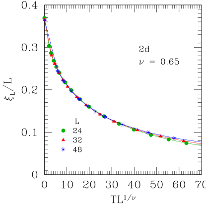
Figure 13: A scaling plot of the data from the largest sizes for $\xi_{L}/L$ in two dimensions assuming $T_{SG}=0$.

We have also computed the correlation length $\xi_{L}/L$ in two dimensions, and show the data in Fig. (12). The curves become independent of size, for large $L$, at $T=0$, confirming that $T_{SG}=0$. A scaling plot of the data for the largest sizes ($L\geq 24$) in Fig. 13 has the best data collapse with $\nu=0.65$ and altogether we estimate

$$\nu=0.65\pm 0.05\qquad(d=2,\quad\text{from }\xi_{L}/L)\,,$$ (27)

which is consistent with our estimate from ${\chi_{\rm SG}}$ in Eq. (26), and with the result of Morris et al. Morris et al. (1986).

V Conclusions

We have considered the spin glass in the limit where the spins have an infinite number of components. In the formulation of this problem appropriate for numerical calculations Bray and Moore (1982); Morris et al. (1986); Hastings (2000); Aspelmeier and Moore (2004), where the limit $m\to\infty$ is taken with $N$ finite, we find that the order parameter, defined in terms of correlation functions in zero (symmetry-breaking) field, vanishes. Instead, below $T_{SG}$, there is only “quasi-long range order” in which the correlations decay to zero with a power of distance. Whereas we define the order parameter in terms of the the long distance limit of the correlation functions, Aspelmeier and Moore Aspelmeier and Moore (2004) define a local order parameter in terms of the contribution to the constraint in Eq. (6) that comes from the eigenmodes with zero eigenvalue of the matrix $A_{ij}$. They argue their order parameter is related to the susceptibility in the presence of a small field $h$, where the limit $N\to\infty$ is taken before the limit $h\to 0$ in order to break the symmetry. From numerics on the infinite-range model, Aspelmeier and Moore claim that their order parameter agrees with that of Almeida et al. de Almeida et al. (1978).

However, in a sensible physical model, any reasonable definition of the order parameter should give the same answer. In particular, one should be able to obtain the square of the order parameter from the long distance limit of the correlation function (off-diagonal long range order) in zero field, and get the same answer as the local expectation value of the spin in the presence of a small symmetry breaking field. This does not appear to be the case for the $m=\infty$ model if the limit $m\to\infty$ is taken before $N\to\infty$.

On the other hand, if the thermodynamic limit, $N\to\infty$, is taken with $m$ large but finite, then the correlations saturate at a value of order $1/m$ at large distance, and so a finite spin glass order parameter can be defined from the long distance limit of the correlation functions. This seems to agree with that found in the analytical work of Ref. [de Almeida et al., 1978], and is presumably the same as the local order parameter in a symmetry breaking field. Hence, there seems to be no inconsistency if the limit $N\to\infty$ is taken first.

We have also studied the $m=\infty$ model in three dimensions, finding the transition to be at zero temperature, in contrast to the situation for Ballesteros et al. (2000); Lee and Young (2003) $m=1,2$ and $3$. We suspect that $T_{SG}=0$ only in the $m=\infty$ limit, rather than for all $m$ less than some (non-zero) critical value $m_{c}$, since spin glasses with $m=\infty$ seem to have unique features. We have already mentioned that there is only quasi long-range order below $T_{SG}$ in this case, in contrast to finite-$m$. Another example is that Green et al. Green et al. (1982) find the upper critical dimension, above which the critical exponents are mean field like, to be $d_{u}=8$, whereas for finite $m$ one has $d_{u}=6$. Our result that $T_{SG}=0$ for $m=\infty$ in $d=3$ is consistent with the claim of Viana Viana (1988) that that the lower critical dimension (below which $T_{SG}=0$) is also $d_{l}=8$, but currently we cannot say anything specific about dimensions above 3.

We find, not surprisingly, that $T_{SG}=0$ also in two dimensions. Our results for the correlations length exponent at the $T=0$ transition in $d=2$ and 3 are consistent with those of Morris et alMorris et al. (1986).

Finally, we note that Aspelmeier and Moore Aspelmeier and Moore (2004) have proposed that the $m=\infty$ model is a better starting point for describing Ising or Heisenberg spin glasses in finite dimensions, than the Ising model. We have argued in this paper that the spin glass with $m$ strictly infinite is not a sensible model, but one rather needs to consider $m$ large but finite. Hence, the $m=\infty$ formulation proposed by Aspelmeier and Moore Aspelmeier and Moore (2004) and others Bray and Moore (1982); Morris et al. (1986); Hastings (2000) would need to be extended to a $1/m$ expansion and evaluated, at the very least, to order $1/m$. More probably an infinite resummation would be needed (M. A. Moore, private communication) to obtain sensible results in the spin glass phase, but this may be feasible.