Pair Contact Process with Diffusion: Failure of Master Equation Field Theory

Abstract

We demonstrate that the ‘microscopic’ field theory representation, directly derived from the corresponding master equation, fails to adequately capture the continuous nonequilibrium phase transition of the Pair Contact Process with Diffusion (PCPD). The ensuing renormalization group (RG) flow equations do not allow for a stable fixed point in the parameter region that is accessible by the physical initial conditions. There exists a stable RG fixed point outside this regime, but the resulting scaling exponents, in conjunction with the predicted particle anticorrelations at the critical point, would be in contradiction with the positivity of the equal-time mean-square particle number fluctuations. We conclude that a more coarse-grained effective field theory approach is required to elucidate the critical properties of the PCPD.

I Introduction

Phase transitions between different nonequilibrium steady states are frequently encountered in nature, and determining the associated critical properties is an important issue. Unfortunately, compared with the situation in thermal equilibrium, a full classification of nonequilibrium phase transitions is still in its infancy. We shall focus here on a particular subclass of nonequilibrium transitions which separate an ‘active’ phase, characterized by a fluctuating order parameter $\phi(\mathbf{r},t)$ with nonzero average $\langle\phi\rangle$, from an absorbing state wherein $\langle\phi\rangle=0$. In the thermodynamic limit, all degrees of freedom remain strictly frozen in such an inactive, absorbing phase books .

The universality classes of such transitions are conveniently studied in the framework of reaction-diffusion processes, even though other descriptions abound (surface growth, self-organized criticality) hinrichsenodorrev . The most prominent representative of absorbing state transitions is the contact process (CP), for under quite generic conditions, namely spatially and temporally local microscopic dynamics, and the absence of coupling to other slow fields (thus excluding quenched disorder and the presence of conservation laws), active to absorbing state transitions fall into the CP universality class with scaling exponents that also describe critical directed percolation (DP) clusters janssen ; grassberger . Yet, the very fact that despite considerable effort hardly any experiments have to date unambiguously identified the CP/DP critical exponents, hints at the prevalence of other universality classes. In simulations, the ‘parity-conserving’ (PC) universality class is also prominent: represented by one-dimensional branching and annihilating random walks (BAW) $A\to(m+1)\,A$, $A+A\to\emptyset$ with even $m$, it is characterized by local particle number parity conservation. In contrast, the phase transition in low-dimensional BAW with odd $m$ is governed by DP exponents hinrichsenodorrev ; johnuwe .

Novel critical behavior is to be expected when all involved reactions require the presence of neighboring particle pairs grassberger . The pair contact process with diffusion (PCPD, or annihilation/fission model martinuwe ) is conveniently defined through the microscopic reaction rules

$$A+A\stackrel{{\scriptstyle\mu}}{{\to}}\emptyset\,,\quad A+A\stackrel{{\scriptstyle\mu^{\prime}}}{{\to}}A\,,\quad A+A\stackrel{{\scriptstyle\sigma}}{{\to}}A+A+A\quad$$ (1)

(the presence of either pair annihilation $\sim\mu$ or coagulation $\sim\mu^{\prime}$ suffices), supplemented with particle hopping (diffusion constant $D$) subject to mutual exclusion. The latter is crucial for the existence of a well-defined active phase and continuous transition. For without restrictions on the occupation number per lattice site, the particle density diverges within a finite time when $\sigma>\sigma_{c}=2\mu+\mu^{\prime}$ martinuwe . In the inactive phase, however, site exclusion should not be relevant. It is then easily seen that the absorbing state of the PCPD (as in the PC universality class johnuwe ) is governed by the algebraic density decay of the pure pair annihilation process pelitilee , viz. $\langle\phi(t)\rangle\sim t^{-1}$ in dimensions $d>2$, $\langle\phi(t)\rangle\sim t^{-d/2}$ for $d<2$, and $\langle\phi(t)\rangle\sim t^{-1}\ln t$ at the (upper) critical dimension $d_{c}=2$. In contrast, in the CP/DP universality class, the inactive phase is characterized by exponential particle decay and correlations. Recall that here the branching processes merely require the presence of a single particle: the third reaction in (1) would simply be replaced with $A\to A+A$. Site exclusion is not crucial in this case, as long as the pair annihilation or coagulation reactions are included. Alternatively, the combined first-order reactions $A\to\emptyset$ and $A\to A+A$ with site exclusion yield a CP/DP continuous phase transition as well.

Holding the rates $\mu$ and $\mu^{\prime}$ fixed, there is a critical production rate $\sigma_{c}$ at which the transition between the active nonequilibrium steady state and the absorbing phase occurs. It is a central issue, in an effort to classify nonequilibrium phase transitions, to clarify the precise manner in which the particle production mechanism defines the properties of both the absorbing state and the universality class of the transition, i.e., how it affects scaling properties in the vicinity of the critical point. Numerical investigations of the PCPD started with Ref. carlonhenkelschollwoeck . It almost constitutes an euphemism to state that this and the subsequent flurry of numerical work hinrichsen1 –nohpark have revealed conflicting views (see Ref. henkelhinrichsen for a comprehensive overview): For not only are the precise numerical values of the critical exponents still being debated to this day, but even more striking, the very issue of the PCPD universality class has remained controversial. Essentially three scenarios have been put forward: Either the transition defines a novel independent universality class that is yet to be characterized, or it belongs to the CP/DP, or even to the PC class (the latter perhaps becoming less likely with improving simulation accuracy). In addition, the emergence of different scaling properties depending on the value of the diffusion rate has been claimed.

This inconclusive numerical situation clearly calls for analytical approaches to provide further understanding of the elusive continuous phase transition of the PCPD with restricted particle occupation numbers. A natural starting point is the standard field-theoretic representation of reaction-diffusion systems that can be derived directly from the corresponding classical master equation doietal . Specifically, dynamical renormalization group (RG) studies based on such ‘microscopic’ field theories were, e.g., successfully employed to diffusion-limited annihilation pelitilee and even-offspring BAW johnuwe , as well as the inactive phase of the PCPD without site occupation restrictions martinuwe . In either case, particle anticorrelations govern the asymptotic scaling regime, as opposed to the typical clustering behavior in the CP/DP universality class (that includes odd-offspring BAW) janssen . Here another coarse-graining step takes the original ‘microscopic’ master equation representation to Reggeon field theory, equivalent to a Langevin equation with ‘square-root’ multiplicative noise, that serves as the appropriate effective action for the CP/DP critical properties. Thus, one would hope that the continuous nonequilibrium phase transition in the PCPD with restricted site occupations should be amenable to these powerful tools as well.

Yet it was only recently demonstrated how site exclusions can be consistently incorporated into the master equation field theory formalism fredo . This paper reports our study of the ensuing action for the PCPD, constructed in Sec. II, carefully taking into account the higher-order reactions that become generated through fluctuations, i.e., successive particle production processes martinuwe . We shall derive and discuss the ensuing RG flow equations in Sec. III. We will demonstrate that there exists in fact no stable RG fixed point in the physically accessible parameter space of the model (wherein all reaction rates are non-negative). Remarkably therefore, the microscopic field theory, albeit directly derived from the master equation, is not capable of capturing the PCPD critical point. We interpret the appearance of runaway flows as an indication that a crucial ingredient was obviously left out when the (naive) continuum limit was taken fnote1 . An appropriate effective coarse-grained description might require the explicit introduction of separate density fields for the ‘inert’ solitary random walkers and the clustered particles, respectively, akin to the explicit treatment of particle pairs and singlets in Ref. hinrichsen2 . The RG flow equations do however allow for a fixed point outside the physical region. In Sec. IV we compute the associated critical exponents to second order in an expansion around the upper critical dimension $d_{c}=2$, and moreover establish exact scaling relations. But we shall see that the actual exponent values, when combined with the predicted particle anticorrelations at the critical point, violate the positivity of the equal-time mean-square particle fluctuations. Hence this RG fixed point is clearly unphysical. In conclusion, the construction of a consistent field theory description of the PCPD remains an open problem. Similar issues arise also for the closely related models that involve solely particle triplet or quadruplet reactions parkhinrichsenkim2 ; kockelkorenchate1 ; odor4 .

II Master equation field theory representation of the PCPD

The classical master equation kinetics of particles subject to diffusion and local ‘chemical’ reactions can be mapped onto a field theory action following standard procedures doietal ; pelitilee . However, for the density to remain bounded in the processes (1) at arbitrary values of the reaction rates, specifically in the active phase, it is necessary to introduce a growth-limiting process. In most numerical simulations this is achieved by further imposing mutual exclusion between particles. Analytical progress therefore requires a consistent incorporation of the exclusion constraint. To this end, we follow Ref. fredo , and write down the resulting action corresponding to the processes (1) on a (for the sake of notational simplicity one-dimensional) lattice (sites $i$):

$$S[\{{\hat{\phi}}_{i},\phi_{i}\}]=\sum_{i}\int\!dt\ \Biggl{(}{\hat{\phi}}_{i}\,\partial_{t}\phi_{i}+\biggl{\{}\mu\left({\hat{\phi}}_{i}\,{\hat{\phi}}_{i+1}-1\right)$$

$$\qquad\qquad\qquad+\frac{\mu^{\prime}}{2}\left[\left({\hat{\phi}}_{i}-1\right){\hat{\phi}}_{i+1}+\left({\hat{\phi}}_{i+1}-1\right){\hat{\phi}}_{i}\right]$$

$$\,+\frac{\sigma}{2}\left[\left(1-{\hat{\phi}}_{i-1}\right)e^{-{\hat{\phi}}_{i-1}\phi_{i-1}}+\left(1-{\hat{\phi}}_{i+2}\right)e^{-{\hat{\phi}}_{i+2}\phi_{i+2}}\right]$$

$$\qquad\qquad\quad\times\ {\hat{\phi}}_{i}{\hat{\phi}}_{i+1}\biggr{\}}\ \phi_{i}\,\phi_{i+1}\ e^{-{\hat{\phi}}_{i}\phi_{i}-{\hat{\phi}}_{i+1}\phi_{i+1}}\Biggr{)}\ .$$ (2)

The time-dependent fields ${\hat{\phi}}_{i}(t)$ and $\phi_{i}(t)$ here originate from a coherent-state representation employing bosonic creation and annihilation operators doietal ; pelitilee . The exclusion constraints are encoded in the exponential terms fredo , and the unrestricted model is recovered when all these exponentials are replaced with unity.

Thus far, the action (II) constitutes an exact representation of the microscopic processes (1). In order to proceed to a continuum field theory, which should suffice to describe the large-scale, long-time behavior in the vicinity of a critical point, we add a diffusion term (for which we ignore the site occupation restrictions fnote2 ) and take the (naive) continuum limit (now in $d$ dimensions) ${\hat{\phi}}_{i}(t)\to{\hat{\phi}}(\mathbf{r},t)$ and $\phi_{i}(t)\to a^{d}\phi(\mathbf{r},t)$, with $a$ denoting the original lattice spacing, such that ${\hat{\phi}}(\mathbf{r},t)$ remains dimensionless. This yields

$$S[{\hat{\phi}},\phi]=\int\!d^{d}x\int\!dt\ \biggl{\{}{\hat{\phi}}\left(\partial_{t}-D\,\nabla^{2}\right)\phi$$

$$\qquad\qquad\quad-\Bigl{[}\mu\left(1-{\hat{\phi}}^{2}\right)+\mu^{\prime}\left(1-{\hat{\phi}}\right){\hat{\phi}}\Bigr{]}\phi^{2}\ e^{-2v\,{\hat{\phi}}\phi}$$

$$\qquad\qquad\qquad+\sigma\left(1-{\hat{\phi}}\right){\hat{\phi}}^{2}\,\phi^{2}\ e^{-3v\,{\hat{\phi}}\phi}\biggr{\}}\ ,$$ (3)

with a microscopic inverse density scale $v\sim a^{d}$.

The corresponding classical rate equation (augmented with diffusion) is readily obtained by solving for the stationarity conditions $\delta S[{\hat{\phi}},\phi]/\delta\phi=0$, which, as a consequence of probability conservation in the master equation, is always satisfied by ${\hat{\phi}}=1$, and $\delta S[{\hat{\phi}},\phi]/\delta{\hat{\phi}}=0$, which then results in

$$\left(\partial_{t}-D\,\nabla^{2}\right)\phi(\mathbf{r},t)=\phi^{2}\left[\sigma-\left(2\mu+\mu^{\prime}\right)e^{v\,\phi}\right]e^{-3v\,\phi}\ .$$ (4)

In contrast with the unrestricted model (where $v=0$), this mean-field equation allows for an active state with a finite particle density $\phi=v^{-1}\ln(\sigma/\sigma_{c})$, provided $\sigma>\sigma_{c}=2\mu+\mu^{\prime}$. Near the now well-defined critical point at $\sigma_{c}$, we obtain

$$\phi(\sigma)\approx v^{-1}[(\sigma/\sigma_{c})-1]\sim(\sigma-\sigma_{c})^{\beta}\ ,\quad\beta=1\ .$$ (5)

In the absorbing phase ($\sigma<\sigma_{c}$), the site restrictions do not matter, and the density decays algebraically as in pure annihilation or coagulation, $\phi(t)\sim[(\sigma_{c}-\sigma)t]^{-1}$. At the critical point, this becomes replaced with the slower power law

$$\phi(t)\sim(v\sigma_{c}\,t)^{-1/2}\sim t^{-\delta}\ ,\quad\delta=1/2\ .$$ (6)

This relation already shows that the scaling of the parameter $v$ determines the critical exponents. Moreover, scaling analysis tells us that the static correlation length diverges upon approaching the critical point from the active side according to $\xi(\sigma)\sim(\sigma-\sigma_{c})^{\nu}$ with $\nu=1$, whereas the characteristic time scales as $t_{c}\sim\xi^{z}$ with diffusive dynamic critical exponent $z=2$.

While we clearly need to retain the exclusion parameter in order to describe the continuous phase transition occuring at $\Delta\propto\sigma-\sigma_{c}=0$, we also note that an expansion to first order in $v$ suffices. More technically, since the field $\phi(\mathbf{r},t)$ scales as a particle density, the scaling dimension of the exclusion parameter is $[v]=\kappa^{-d}$, where $\kappa$ represents an arbitrary momentum scale. Superficially, therefore, $v$ constitutes an irrelevant coupling that flows to zero under scale transformations. We may thus expand the exponentials in the action (II), keeping only the lowest-order contributions, which leads to additional interaction terms. Upon at last performing the field shift ${\hat{\phi}}(\mathbf{r},t)=1+\bar{\phi}(\mathbf{r},t)$ (whereby final-time contributions, not explicitly listed here, become eliminated fnote3 ), we arrive at an action of the form

$$S[\bar{\phi},\phi]=\int\!dx\int\!dt\ \Bigl{[}\bar{\phi}\left(\partial_{t}-D\,\nabla^{2}\right)\phi+G(\bar{\phi})\,\phi^{2}$$

$$\qquad\qquad\qquad\qquad\qquad+\Lambda(\bar{\phi})\,\phi^{3}+\ldots\Bigr{]}\ ,$$ (7)

where we have defined the generating functions

$$G(x)=\sum_{p\geq 1}g_{p}\,x^{p}\,,\quad\Lambda(x)=\sum_{p\geq 1}\lambda_{p}\,x^{p}\ .$$ (8)

Note that probability conservation implies $G(0)=0$ and $\Lambda(0)=0$. Microscopically, we identify $g_{1}=2\mu+\mu^{\prime}-\sigma=\sigma_{c}-\sigma$, $g_{2}=\mu+\mu^{\prime}-2\sigma$, $g_{3}=-\sigma$, $\lambda_{1}=(3\sigma-4\mu-2\mu^{\prime})v$, $\lambda_{2}=(9\sigma-6\mu-4\mu^{\prime})v$, $\lambda_{3}=(9\sigma-2\mu-2\mu^{\prime})v$, and $\lambda_{4}=3\sigma\,v$. However, at a coarse-grained level, fluctuations generate the entire sequence of particle production reactions $2A\to(n+2)A$ ($n\geq 1$). For instance, two subsequent branching processes $2A\to 3A$ immediately lead to $2A\to 4A$, and so forth martinuwe . This effectively extends the sums in the functions (8) to all integer $p$. Unlike in conventional situations, we thus have to deal with an infinite number of vertices. Lastly we remark that introducing third-order annihilation reactions of the form $3A\to kA$ ($k=0,1,2$) also produces the terms in the second line of Eq. (II): Allowing for the back reactions of the particle production processes is equivalent to ‘soft’ site exclusions.

With the previously introduced scaling dimensions of the fields $[\bar{\phi}]=\kappa^{0}$ and $[\phi]=\kappa^{d}$, we find $[g_{p}]=\kappa^{2-d}$ for all couplings in $G(x)$, which suggests, as is then confirmed by a careful analysis of Feynman diagrams, that $d_{c}=2$ constitutes the upper critical dimension here. Since $[\lambda_{p}]=\kappa^{2(1-d)}$, the coefficients in the function $\Lambda(x)$, which originates from site exclusion, are irrelevant near $d_{c}=2$. Yet because at least $\lambda_{1}$ is required to control the particle density in the active phase and thereby maintain a continuous transition, it cannot simply be omitted from (II). Once again though we arrive at the conclusion that terms of higher order in $v$ (i.e., contributions $\sim\phi^{4}$ or higher in the action) need not be retained. But despite the presence of apparently infinitely many marginal couplings, the field theory (II) remains renormalizable. This is best seen by recalling that the choice of the scaling dimensions for the fields is actually arbitrary as long as the product $[\bar{\phi}\,\phi]=\kappa^{d}$. Our theory thus contains a redundant variable wegner that we fix conveniently as follows: Upon introducing recaled fields $\bar{s}=\kappa^{d/2}\bar{\phi}$ and $s=\kappa^{-d/2}\phi$, we obtain $[g_{p}]=\kappa^{2-p\,d/2}$ and $[\lambda_{p}]=\kappa^{2-(p+1)d/2}$. Consequently, the critical control parameter constitutes a relevant perturbation (for $d<4$), since $[g_{1}]=\kappa^{2-d/2}$, whereas $[g_{2}]=[\lambda_{1}]=\kappa^{2-d}$ indicating that both $g_{2}$ and $\lambda_{1}$ are marginal at $d_{c}=2$. Indeed, this procedure is consistent with the critical behavior according to Eq. (6) in two dimensions, which requires the density to scale $\sim t^{-1/2}\sim\kappa$ rather than $\sim t^{-1}\sim\kappa^{2}$ which is valid in the absorbing phase. All other couplings now acquire negative scaling dimensions, and therefore become irrelevant for the leading scaling behavior. This leaves us with the reduced action

$$S[\bar{s},s]=\int\!dx\int\!dt\ \Bigl{[}\bar{s}\left(\partial_{t}-D\,\nabla^{2}\right)s+g_{1}\,\bar{s}\,s^{2}$$

$$\qquad\qquad\qquad\qquad\qquad+g_{2}\,\bar{s}^{2}s^{2}+\lambda_{1}\,\bar{s}\,s^{3}\Bigr{]}\ .$$ (9)

Thus, the appropriate effective field theory for the critical point in fact only contains three nonlinear vertices.

III Renormalization and RG flow

It is instructive to proceed with the renormalization program based on either the field theory (II) with infinitely many marginal couplings and the reduced action (II). One immediately notices that, to all orders in the perturbation expansion, the propagators do not become renormalized. Hence there is neither field nor diffusion constant renormalization, which already implies that the dynamic exponent in these field theories inevitably remains $z=2$ exactly, at variance with present simulation data. Next, for the action (II) we define renormalized parameters according to $g_{p}\,C_{\epsilon}=Z_{p}\,g_{p{\rm R}}\,D\,\kappa^{\epsilon}$, and $\lambda_{p}\,C_{\epsilon}=Z_{\lambda_{p}}\,\lambda_{p{\rm R}}\,D\,\kappa^{-2+2\epsilon}$ with $C_{\epsilon}=(4\pi)^{-d/2}\,\Gamma(1+\epsilon/2)$. The renormalization constants $Z_{p}$ and $Z_{\lambda_{p}}$ are determined by means of dimensional regularization and minimal subtraction by the condition that they absorb just the ultraviolet divergences appearing as poles in $\epsilon=2-d$. After computing the RG $\beta$ functions $\beta_{p}=\kappa\,\partial_{\kappa}g_{p{\rm R}}$ (evaluated in the unrenormalized theory) and upon introducing the flow parameter $\ell=-\ln(\kappa a)$ (where $\kappa$ is the running momentum scale), we subsequently obtain the corresponding RG flow equations for the running couplings, $\partial_{\ell}\,g_{p{\rm R}}(\ell)=-\beta_{p}(\ell)$, and similarly for the $\lambda_{p{\rm R}}$.

We start with renormalizing the action (II). The vertex $\sim\lambda_{1}$ does not enter any Feynman diagrams that contribute to the renormalization of $g_{1}\,C_{\epsilon}=Z_{1}\,g_{1{\rm R}}\,D\,\kappa^{1+\epsilon/2}$ and $g_{2}\,C_{\epsilon}=Z_{2}\,g_{2{\rm R}}\,D\,\kappa^{\epsilon}$. For the latter, we are therefore left with precisely the structure of the pure annihilation / coagulation field theory pelitilee , namely a geometric series of one-loop graphs, and hence arrive at the exact result

$$Z_{1}^{-1}=Z_{2}^{-1}=1-\frac{2\,g_{2{\rm R}}}{\epsilon}\ .$$ (10)

This leaves $Z_{\lambda_{1}}$ in $\lambda_{1}\,C_{\epsilon}=Z_{\lambda_{1}}\,\lambda_{1{\rm R}}\,D\,\kappa^{\epsilon}$ as the sole renormalization constant to be actually determined anew here. To two-loop order, we find fnote4

$$Z_{\lambda_{1}}^{-1}=1-\frac{6\,g_{2{\rm R}}}{\epsilon}+\frac{12\,g_{2{\rm R}}^{2}}{\epsilon^{2}}\left(1+\frac{\epsilon}{2}\,\ln\frac{4}{3}\right)\,.$$ (11)

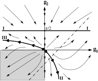
Figure 1: Qualitative flow diagram of the RG trajectories in the ($g_{1},g_{2}$)-plane. I denotes the stable fixed line; II and III represent the parts of the separatrix that might collapse in the limiting case with the negative half-axes. The hatched area indicates the absolutely unstable region. The dash-dotted line corresponds to the initial values of the model, with $2g_{1}-g_{2}={\rm const.}>0$.

From Eqs. (10) we obtain the RG flow equations

$$\partial_{\ell}\,g_{1/2{\rm R}}(\ell)=\bigl{[}\epsilon-2\,g_{2{\rm R}}(\ell)\bigr{]}\,g_{1/2{\rm R}}(\ell)\ .$$ (12)

It follows that the sign of $g_{1{\rm R}}$ is invariant under the RG flow, and the critical $g_{1{\rm R}}=0$ remains fixed. If both $g_{1{\rm R}}$ and $g_{2{\rm R}}$ are negative, the flow according to Eqs. (12) leads both running couplings towards $-\infty$ (‘Wilson’s gully’). Only if either parameter is initially positive, can the stable fixed line with arbitrary $g_{1{\rm R}}$ and $g_{2{\rm R}}^{*}=\epsilon/2$ be reached. Thus, a separatrix must exist between the fully unstable region in parameter space and the basin of attraction of the fixed line. A qualitative sketch of the ensuing RG trajectories is depicted in Fig. 1.

Before we proceed further with a discussion of the RG flow trajectories, let us consider the field theory (II), and for the moment omit the irrelevant parameters $\lambda_{p}$. One is then concerned with controlling the infinite number of marginally relevant vertices $g_{p}$. This is most elegantly achieved by introducing the renormalized counterpart of the generating function $G_{\rm R}(x)=\sum_{p\geq 1}g_{p{\rm R}}\,x^{p}$ john . As anticipated, a careful analysis of the appropriate Feynman diagrams indeed shows that not only are the renormalizations of the $g_{p}$ interwined, but also such couplings of arbitrarily high order become generated. For example, an explicit two-loop calculation results in

$$\!Z_{2}^{-1}\!=1-\frac{2g_{2}\,C_{\epsilon}\kappa^{-\epsilon}}{D\,\epsilon}-\frac{6g_{1}g_{3}\,C_{\epsilon}\kappa^{-\epsilon}}{Dg_{2}\,\epsilon}+\frac{24g_{1}^{2}g_{4}C_{\epsilon}^{2}\kappa^{-2\epsilon}}{D^{2}\,g_{2}\,\epsilon^{2}}$$

$$\ +\frac{4g_{2}^{2}\,C_{\epsilon}^{2}\kappa^{-2\epsilon}}{D^{2}\,\epsilon^{2}}+\frac{12g_{1}g_{3}\,C_{\epsilon}^{2}\kappa^{-2\epsilon}}{D^{2}\,\epsilon^{2}}\left(1+\frac{\epsilon}{2}\,\ln\frac{4}{3}\right).$$ (13)

To one-loop order, elementary combinatorics yields martinuwe

$$Z_{p}^{-1}=1-\frac{1}{\epsilon}\,\sum_{j=1}^{p}j(j+1)\ \frac{g_{j+1{\rm R}}\,g_{p-j+1{\rm R}}}{g_{p{\rm R}}}\ ,$$ (14)

whence $\beta_{p}=-\epsilon\,g_{p{\rm R}}+\sum_{j=1}^{p}j(j+1)\,g_{j+1{\rm R}}\,g_{p-j+1{\rm R}}$. The ensuing infinite hierarchy of ome-loop flow equations for the $g_{p{\rm R}}$ is then efficiently recast into a single functional RG differential equation for $G_{\rm R}(x,\ell)$ john :

$$\partial_{\ell}\,G_{\rm R}(x,\ell)=\left[\epsilon-\partial_{x}^{2}\,G_{\rm R}(x,\ell)\right]G_{\rm R}(x,\ell)\ .$$ (15)

Although we shall not explicitly make use of it, one may derive in a similar fashion the one-loop functional RG flow equation for the generating function $\Lambda_{\rm R}$ that incorporates all the couplings induced by the site exclusions:

$$\partial_{\ell}\,\Lambda_{\rm R}(x,\ell)=-2(1-\epsilon)\,\Lambda_{\rm R}(x,\ell)$$ (16)

$$\ -G_{\rm R}(x,\ell)\ \partial_{x}^{2}\,\Lambda_{\rm R}(x,\ell)-3\,\Lambda_{\rm R}(x,\ell)\ \partial_{x}^{2}\,G_{\rm R}(x,\ell)\ .$$

Recall that the initial generating function was a third-order polynomial $G_{0{\rm R}}(x)=g_{1{\rm R}}\,x+g_{2{\rm R}}\,x^{2}+g_{3{\rm R}}\,x^{3}$ with at least $g_{3{\rm R}}<0$. Upon setting the right-hand side of Eq. (15) to zero, we find the locally stable nontrivial fixed-point function

$$G_{\rm R}^{*}(x)=\Delta\,x+\frac{\epsilon}{2}\,x^{2}$$ (17)

with arbitrary constant $\Delta$, whereas the trivial solution $G_{\rm R}^{*}=0$ is clearly unstable. This result is in fact valid to all orders in $\epsilon$ fnote5 . Therefore, all running couplings $g_{p{\rm R}}(\ell)\to 0$ for $p\geq 3$, and we recover the results (10), (11), and (12) previously obtained from the reduced action (II). As anticipated, $\Delta$, the renormalized counterpart to $g_{1}$, plays the role of a control parameter, albeit not a relevant one, since that would have to scale to infinity under renormalization rather than remain constant. We assume that $\Delta$ is a regular function of the initial rates; i.e., at fixed annihilation and coagulation rates we expand for $\sigma\to\sigma_{c}$: $\Delta(\sigma)\simeq(\sigma_{c}-\sigma)\,\Delta^{\prime}(\sigma_{c})$, since $\Delta(\sigma_{c})=0$ and $\Delta^{\prime}(\sigma_{c})>0$. Indeed, the pure annihilation and coagulation model fixed points at $\sigma=0$ respectively correspond to $\Delta=\epsilon$ (since $g_{1}=2g_{2}$) and $\Delta=\epsilon/2$ ($g_{1}=g_{2}$) pelitilee . Thus, in the PCPD inactive phase $\sigma<\sigma_{c}$ one should have $\Delta={\cal O}(\epsilon)>0$ as well. Notice that at $\sigma_{c}=2\mu+\mu^{\prime}$ we have $g_{2}=-3\mu-\mu^{\prime}$, hence this combination of annihilation and coagulation rates has apparently turned negative at the fixed point. One must therefore worry whether the physically accessible values of the reaction rates actually lie within the basin of attraction of the nontrivial fixed-point function $G_{\rm R}^{*}(x)$.

Thus we now resume our discussion of the RG trajectories. On physical grounds one should expect that the flow would at least reach the line of fixed points encoded by Eq. (17) if $g_{1{\rm R}}$ is positive, since this corresponds to the inactive phase governed by the annihilation / coagulation fixed line. Yet for this to be true for any $g_{1{\rm R}}>0$, the part of the separatrix indicated by II in Fig. 1 must collapse onto the negative $g_{2}$-axis, i.e., the separatrix should contain the invariant hypersurface $g_{1}=0$. This would indeed lead to the standard RG flow picture: With initial values corresponding to the inactive phase the RG trajectories approach the annihilation / coagulation fixed line, critical initial conditions are defined by the separatrix (which is unstable along one direction), and finally initial values corresponding to the active phase are to be found inside the unstable region with flow into the ‘gully’.

Yet it is easily seen that the zeros $x_{i}$ with $G_{\rm R}(x_{i},\ell)=0$ are fixed by the partial differential equation (15), and consequently also the intervals in which the function $G_{\rm R}(x,\ell)$ is respectively positive or negative. Therefore, if (i) $g_{1{\rm R}}>0$, there exists an open interval $(x_{0}=0,x_{1}>0)$ wherein $G_{\rm R}(x,\ell)>0$, while $G_{\rm R}(x_{0,1},\ell)=0$. Since initially $g_{3{\rm R}}<0$, however, it follows that the fixed-point function (17) cannot be reached from the physically allowed region in parameter space. This is true for arbitrary values of $\Delta$ and for all $-\infty<x<\infty$, even if $g_{2\rm R}>0$. This is rather astonishing because one would expect that at least deep in the inactive phase, where the production reactions can be neglected, $G_{\rm R}(x,\ell)\to G_{\infty}(x)=G_{\rm R}^{*}(x)$ as $\ell\to\infty$ for all $x$. It is however obvious that we can assume this limiting relation to hold only in the first positive interval in an expansion of $G_{\rm R}(x)$ with respect to $x$. We conclude that the difference function $H(x)=G_{\rm R}^{*}(x)-G_{\infty}(x)$ must display an essential singularity at $x=0$, and its expansion in a series of $x$ produces simply a zero. However, $H(x_{1})=G_{\rm R}^{*}(x_{1})$. A qualitative discussion of the differential equation (15) indeed supports this assumption. Note here that $G_{\rm R}(x,\ell)$ increases most significantly with $\ell$ at those values of $x$ where its curvature is minimal. (ii) In the case $g_{1{\rm R}}\leq 0$ the initial function is negative for all $x>0$. Hence the differential equation (15) does not provide any mechanism that could translate $G_{\rm R}(x,\ell)$ to positive values and finally to $G_{\rm R}^{*}(x)$, at least in some $x$-intervals, without producing zeros of $G_{\rm R}(x)$ along the way. In summary, we find that our physical initial conditions at the critical point (with $g_{3{\rm R}}<0$ as well as $g_{2{\rm R}}<0$ for $g_{1{\rm R}}=\Delta=0$) inevitably take the RG flow from Eq. (15) into the absolutely unstable region in Fig. 1. Instead of reaching the stable fixed line (17), we face runaway trajectories, to all orders in the perturbation expansion.

IV Critical properties at the unphysical fixed point

Even though we have just seen that the critical fixed point $g_{1{\rm R}}=\Delta=0$ and $g_{2{\rm R}}^{*}=\epsilon/2$ is inaccessible to the RG flow trajectories starting at physical initial parameter values (i.e., positive reaction rates), let us nevertheless explore the (hypothetical) ensuing critical behavior. Recall that in the PCPD, totally neglecting particle exclusion, as encoded in the parameter $\lambda_{1}$, suppresses the finite-density steady-state. Hence we retain this (apparently irrelevant) coupling, and moreover investigate how its RG flow towards zero becomes renormalized through fluctuations. From the explicit two-loop result for the associated renormalization constant (11), we may immediately compute the anomalous dimension

$$\gamma_{\lambda_{1}}=\kappa\,\frac{d\ln Z_{\lambda_{1}}}{d\kappa}=-3\,\epsilon+3\,\epsilon^{2}\,\ln\frac{4}{3}+{\cal O}(\epsilon^{3})\ .$$ (18)

As is easily seen by investigating the RG equations for the particle density and its correlation function, $\gamma_{\lambda_{1}}$ already completely determines the critical exponents here. This assertion is also confirmed by directly computing the renormalized equation of state (upon approaching the transition from the active side). For $\Delta\sim\sigma-\sigma_{c}\geq 0$, i.e. in the active phase, one finds that the steady-state density vanishes as $\Delta\to 0^{-}$ according to $\langle\phi\rangle\sim|\Delta|^{\beta}$, with

$$\beta=\frac{1+\gamma_{\lambda_{1}}/2}{d-1-\gamma_{\lambda_{1}}/2}$$

$$\quad\simeq 1-2\,\epsilon+\left(1+3\ln\frac{4}{3}\right)\epsilon^{2}+{\cal O}(\epsilon^{3})\ ,$$ (19)

while the two-point function correlation length (finite only in the active phase) diverges as $\xi\sim|\Delta|^{-\nu}$, where

$$\nu^{-1}=d-1-\frac{\gamma_{\lambda_{1}}}{2}\simeq 1+\frac{\epsilon}{2}-\frac{3}{2}\,\epsilon^{2}\,\ln\frac{4}{3}+{\cal O}(\epsilon^{3})\ .$$ (20)

Precisely at the critical point ($\Delta=0$) the particle density decays asymptotically as $\langle\phi(t)\rangle\sim t^{-\delta}$, with

$$\delta=\frac{1}{2}+\frac{\gamma_{\lambda_{1}}}{4}\simeq\frac{1}{2}-\frac{3}{4}\,\epsilon+\frac{3}{4}\,\epsilon^{2}\,\ln\frac{4}{3}+{\cal O}(\epsilon^{3})\ .$$ (21)

Since remarkably the anomalous fluctuation conrrections to the critical exponents $\beta$, $\nu$, and $\delta$ are solely contained in the anomalous dimension (18), we may eliminate the latter to yield the following hyperscaling relations, valid to all orders in $\epsilon=2-d$:

$$2\,\delta+1/\nu=d\ ,\quad\beta=2\delta/(d-2\delta)=d\,\nu-1\ .$$ (22)

Here we have used the exact result for the dynamic exponent $z=2$ and the standard scaling relation $\beta=z\,\nu\,\delta$ (which also follows directly from the RG equations). At the critical dimension $d_{c}=2$, we infer the asymptotically exact scaling behavior

$$\Delta\to 0^{-}:\ \langle\phi\rangle\sim|\Delta|\,(\ln|\Delta|)^{2}\ ,$$ (24)

$$\ \xi\sim|\Delta|^{-1}\,\big{|}\ln|\Delta|\big{|}^{-1/2}\ ,$$

$$\Delta=0:\ \langle\phi(t)\rangle\sim t^{-1/2}\,(\ln t)^{3/2}\ .$$ (25)

Aside from the fact that these exponent values are at odds with the presently available data from numerical simulations for the PCPD, they also lead to a serious contradiction, which confirms again that the fixed line (17) does not represent a physical system. First, we note that the positive value $g_{2{\rm R}}^{*}=\epsilon/2$ indicates the presence of particle anticorrelations at this fixed point, precisely as in the pure binary annihilation or coagulation system. Next, recall that the equal-time density correlation function of point-like particles consists of three contributions,

$$\langle n(\mathbf{r},t)\,n(\mathbf{r}^{\prime},t)\rangle=\langle n(\mathbf{r},t)\rangle\,\delta(\mathbf{r}-\mathbf{r}^{\prime})$$

$$\quad\qquad+C(\mathbf{r},\mathbf{r}^{\prime};t)+\langle n(\mathbf{r},t)\rangle\,\langle n(\mathbf{r}^{\prime},t)\rangle\ .$$ (26)

The first term here describes the particles’ Poissonian self-correlations. $C(\mathbf{r},\mathbf{r}^{\prime};t)$ represents the density cumulant, i.e., the connected correlation function of the density fluctuations, which is negative in the case of particle anticorrelations. Upon integrating Eq. (IV) over the confining volume and dividing by the mean particle number $\langle N(t)\rangle$, we obtain for a homogeneous state where $C(\mathbf{r},\mathbf{r}^{\prime};t)=C(\mathbf{r}-\mathbf{r}^{\prime};t)$ the following general expression for the relative mean-square particle number fluctuations:

$$\frac{\langle\delta N(t)^{2}\rangle}{\langle N(t)\rangle}=1+\frac{{\widetilde{C}}(t)}{\phi(t)}\ ,$$ (27)

with the mean density $\phi(t)=\langle n(\mathbf{r},t)\rangle$ and the spatial integral of the cumulant ${\widetilde{C}}(t)$.

In the vicinity of a critical point these quantities scale as follows:

$$\phi(t)\sim A\,t^{-\beta/z\nu}\ ,\quad{\widetilde{C}}(t)\sim B\,t^{(d\nu-2\beta)/z\nu}\ .$$ (28)

The amplitude $A$ is of course positive, while $B<0$ in the case of anticorrelations (such as in the PC universality class), and $B>0$ for positive particle correlations (as prevalent in the critical DP clusters). Combining Eqs. (27) and (28) yields

$$\frac{\langle\delta N(t)^{2}\rangle}{\langle N(t)\rangle}\sim 1+\frac{B}{A}\ t^{(d\nu-\beta)/z\nu}\ .$$ (29)

Thus, if $d\nu-\beta>0$ the second term dominates the right-hand side of Eq. (29) asymptotically. For particle anticorrelations where $B/A<0$, this would immediately contradict the positivity of the left-hand side. Consequently, the previously found scaling exponents which satisfy $d\nu-\beta=1$ (exactly) are definitely inacceptable.

This is in remarkable contrast to the results obtained for the pure pair annihilation or coagulation process pelitilee , where the density and the integrated cumulant obey identical asymptotic scaling behavior, $\phi(t)\sim{\widetilde{C}}(t)\sim t^{-d/2}$. Hence no contradiction arises here provided $|B|<A$. Neither are particle anticorrelations necessarily excluded at critical points: For even-offspring BAW that represent the PC universality class, a one-loop RG analysis at fixed dimension yields $\nu=3/(10-3d)$ and $\beta=4/(10-3d)$ johnuwe . Hence $d\nu-\beta\leq 0$ in dimensions $d\leq d_{c}^{\prime}=4/3$, which is precisely the borderline dimension (within the one-loop approximation) for the existence of the phase transition and the power-law inactive phase in this system.

V Conclusions

We have investigated the ‘microscopic’ field theory for the PCPD, as derived directly from the defining master equation, by means of the dynamic renormalization group. Although fluctuations generate an infinite chain of particle production processes $A+A\to(n+2)\,A$, the theory remains controlled and renormalizable in the inactive phase martinuwe , where it is governed by the fixed point of the pure annihilation / coagulation model pelitilee . This is most elegantly seen by means of a functional RG approach john . In order to render the particle density finite in the active phase, we have incorporated site occupation restrictions following the methods developed in Ref. fredo . On the mean-field level, this indeed leads to a continuous transition separating the active from the absorbing phase. However, a detailed analysis of the RG flow equations shows that the action (II) does not adequately capture the critical properties of the PCPD: (i) There is no stable RG fixed point in the physical region of parameter space , and instead one obtains runaway trajectories; (ii) the scaling exponents found at the RG fixed point in the unphysical regime violate the positivity of the mean-square particle number fluctuations.

We emphasize that these statements in fact hold to all orders of the perturbation expansion and even apply to the nonperturbative ‘exact’ RG approach. This failure really resides in the starting field theory action itself, not its subsequent evaluation. Obviously, a crucial ingredient was left out when the ‘naive’ continuum limit was performed. We can only speculate as to what the potential remedies might be, in part motivated by pictures from simulation studies, where positive particle correlations are observed both at the critical point and in the active phase: Perhaps one needs to explicitly introduce separate fields respectively for the positively correlated clustered particles and the solitary random walkers as coupled slow variables. The challenge then, however, is to write down a consistent coarse-grained field theory that correctly accounts for the internal stochastic noise generated by the reactions. To date, therefore, an apt field theory description of the PCPD remains an open and difficult problem.

Finally, we remark that the same problems arise with the master equation field theory when the PCPD order parameter is coupled to a static, conserved background field kockelkorenchate2 . The above statements also apply to active-to-absorbing transitions in related higher-order reactions parkhinrichsenkim2 ; kockelkorenchate1 ; odor4 . For purely triplet reactions, $3A\to mA$ ($m=0,1,2$) and $3A\to(n+3)\,A$ one readily derives a field theory representation corresponding to the action (II), essentially just raising the powers of $\phi$ by one in the nonlinear vertices. In the inactive phase, the theory can again be analyzed by means of the functional RG analogous to Eq. (15), leading to the upper critical dimension $d_{c}=1$, where the particle density decays according to $\langle\phi(t)\rangle\sim(t^{-1}\ln t)^{1/2}$ pelitilee . At the hypothetical critical point one would obtain a slower critical decay $\langle\phi(t)\rangle\sim t^{-1/3}\,(\ln t)^{4/3}$. But once again, the critical fixed point cannot be reached by the RG flow starting at physical parameter values. Moreover, the presence of a redundant parameter even questions the validity of identifying $d=1$ as the critical dimension. Likewise, the expectation that in general fourth-order processes are merely described by mean-field scaling exponents may not be borne out by a correct treatment.

- (1) See, e.g.: J. Marro and R. Dickman, Nonequilibrium phase transitions in lattice models (Cambridge University Press, Cambridge, 1996); B. Chopard and M. Droz, Cellular automaton modeling of physical systems (Cambridge University Press, Cambridge, 1998).
- (2) H. Hinrichsen, Adv. Phys. 49, 815 (2000); G. Ódor, Rev. Mod. Phys. 76, 663 (2004).
- (3) H.K. Janssen, Z. Phys. B 42, 151 (1981).
- (4) P. Grassberger, Z. Phys. B 47, 365 (1982).
- (5) J. Cardy and U.C. Täuber, Phys. Rev. Lett. 77, 4780 (1996); J. Stat. Phys. 90, 1 (1998).
- (6) M.J. Howard and U.C. Täuber, J. Phys. A: Math. Gen. 30, 7721 (1997).
- (7) L. Peliti, J. Phys. A: Math. Gen. 19, L365 (1986); B.P. Lee, J. Phys. A: Math. Gen. 27, 2633 (1994).
- (8) E. Carlon, M. Henkel, and U. Schollwöck, Phys. Rev. E 63, 036101 (2001).
- (9) H. Hinrichsen, Phys. Rev. E 63, 036102 (2001); Physica A 320, 249 (2003); Eur. Phys. J. B 31, 365 (2003).
- (10) H. Hinrichsen, Physica A 291, 275 (2001).
- (11) G. Ódor, Phys. Rev. E 62, R3027 (2000); ibid. 63, 067104 (2001); ibid. 67, 016111 (2003).
- (12) M. Henkel and U. Schollwöck, J. Phys. A: Math. Gen. 34, 3333 (2001).
- (13) K. Park, H. Hinrichsen, and I.-M. Kim, Phys. Rev. E 63, 065103(R) (2001).
- (14) G. Ódor, M.C. Marques, and M.A. Santos, Phys. Rev. E 65, 056113 (2002).
- (15) K. Park and I.-M. Kim, Phys. Rev. E 66, 027106 (2002).
- (16) R. Dickman and M.A.F. de Menezes, Phys. Rev. E 66, 045101(R) (2002).
- (17) J. Kockelkoren and H. Chaté, Phys. Rev. Lett. 90, 125701 (2003).
- (18) G.T. Barkema and E. Carlon, Phys. Rev. E 68, 036113 (2003).
- (19) J.D. Noh and H. Park, Phys. Rev. E 69, 016122 (2004).
- (20) M. Henkel and H. Hinrichsen, J. Phys. A: Math. Gen. 37, R117 (2004).
- (21) M. Doi, J. Phys. A: Math. Gen. 9, 1465 & 1479 (1976); P. Grassberger and P. Scheunert, Fortschr. Phys. 28, 547 (1980); L. Peliti, J. Phys. (Paris) 46, 1469 (1984).
- (22) F. van Wijland, Phys. Rev. E 63, 022101 (2001).
- (23) The equilibrium theory of classical antiferromagnets might provide a useful analogy here: A ‘naive’ continuum limit of the Ising or Heisenberg models directly leads to an action that contains only the local magnetization. In order to describe the physics correctly in terms of an appropriate effective coarse-grained theory, one must first introduce the staggered magnetization as the suitable order parameter, and only then carefully proceed with the continuum limit.
- (24) K. Park, H. Hinrichsen, and I.-M. Kim, Phys. Rev. E 66, 025101(R) (2002).
- (25) G. Ódor, Phys. Rev. E 67, 056114 (2003).
- (26) Implementing the exclusion constraint for the diffusion term as well merely adds irrelevant contributions to the actions (II) and (II).
- (27) Since we retain all powers of , subsequent computations are equivalently carried out in either the shifted or unshifted actions. We have confirmed this through explicit calculations.
- (28) F. Wegner, in Phase Transitions and Critical Phenomena, Vol. 6, eds. C. Domb and M.S. Green (Academic Press, London and New York, 1976).
- (29) Remarkably, an identical two-loop result is found for the anomalous dimension of the branching rate in BAW with johnuwe , albeit based on Feynman diagrams with inverted time arrows.
- (30) J. Cardy, private communication (1997).
- (31) Indeed, even the non-perturbative ‘exact’ RG approach leads precisely to the the functional RG flow equation (15), and consequently to the fixed-point function (17).
- (32) J. Kockelkoren and H. Chaté, e-print cond-mat/0306039.