Vertex dynamics during domain growth in three-state models

Abstract

Topological aspects of interfaces are studied by comparing quantitatively the evolving three-color patterns in three different models, such as the three-state voter, Potts and extended voter models. The statistical analysis of some geometrical features allows us to explore the role of different elementary processes during distinct coarsening phenomena in the above models.

The dynamics of ordering process from a disordered state is a long-standing problem with wide range of application Gunton et al. (1983); Bray (1994). In many cases the growing domains can be characterized by a typical length $r(t)$ (average linear size, correlation length, etc.) for the late stage of coarsening and on the typical length scales the domain structures become similar. The time dependence of the linear length scale can be described by an algebraic growth law, $r(t)\sim t^{n}$ where the growth exponent $n={1\over 2}$ for the curvature-driven growth if the order parameter is not conserved during the elementary processes Allen and Cahn (1979); Bray (1994); Brown and Rikvold (2002).

During the domain growth the interfaces form closed loops in the two-state systems Kadanoff (1976). In the $Q$-state ($Q\geq 3$) systems, however, one can observe vertices where three (or more) states (or interfaces) meet. According to an early conjecture of Lifshitz Lifshitz (1962) and Safran Safran (1981) the curvature driving force for such a domain growth is practically switched off along the straight-line interfaces connecting two vertices and its absence may affect the dynamics of the domain growth. The subsequent numerical investigations of the two-dimensional $Q$-state Potts models did not confirmed this conjecture. More precisely, the first Monte Carlo simulations reported $Q$-dependent effective exponent Sahni et al. (1983b, a), however, the large scale simulation suggested that $n=1/2$ holds independent of the ordering degeneracy, $Q$ Grest et al. (1988). Nevertheless, the numerical evidences to draw any solid conclusions are far from satisfactory. Recently the effects of the branching interfaces during the coarsening process has also been investigated by Cardy Cardy (2000) using a field theoretical approach.

Besides, a distinct universality class, represented by the two-dimensional voter model, is introduced to consider the coarsening process driven by interfacial noises Dornic et al. (2001). In this case the kinetics of domain growth shows a logarithmic decay of the density of interfaces Frachebourg and Krapivsky (1996); Ben-Naim et al. (1996). According to this argument this class is identified by the absence of surface tension.

Motivated by the above mentioned topological aspect, we will consider numerically the time dependence of coarsening process for the three-color growing domain structures. For this purpose we have adopted a numerical technique developed previously to investigate the geometry of spiral structures appearing in some cyclically dominated three-state voter models Szabó and Szolnoki (2002).

In this Brief Report we compare the variation of topological features during the coarsening dynamics in different three-state models. The investigated models are the Potts model, the voter model, and a voter model extended by Potts energy Szabó and Szolnoki (2002). Common feature of these models is the existence of three (equivalent) types of growing domains separated by branching interfaces. The comprehensive comparative geometrical analysis of the topological features allows us to extend the statistical analyses yielding a deeper insight into the kinetics of coarsening.

Henceforth we consider a square lattice (with $L\times L$ sites under periodic boundary conditions) where at each site $x$ there is a state variable with three possible states, namely $s_{x}=0$, $1$, or $2$. The time dependence of these state variables is governed by random sequential updates. Starting from a random initial state this elementary process is repeated. The symmetric elementary rules conserve the equivalence between the three states.

In the case of voter model we choose randomly a nearest neighbor pair of sites and one of these state variables is changed. Variation can only occur if the randomly chosen states are different. More precisely, the different state variables $(s_{1},s_{2})$ become uniform yielding $(s_{1},s_{1})$ or $(s_{2},s_{2})$ pair with equal ($1/2$) probabilities. On the two dimensional lattices this model exhibits coarsening with a logarithmic decay of density of interfaces Frachebourg and Krapivsky (1996); Ben-Naim et al. (1996).

The energy in the three-state ferromagnetic Potts model is defined by the Hamiltonian as

$$H=\sum_{<x,y>}[1-\delta(s_{x},s_{y})]$$ (1)

where the summation runs over the nearest neighbor sites and $\delta(s_{x},s_{y})$ indicates the Kronecker’s delta. On the analogy of the Glauber dynamics, here the state $s_{x}$ at a randomly chosen site $x$ is updated to a new randomly chosen state $s^{\prime}_{x}$. The transition probability is given by

$$W(s_{x}\rightarrow s^{\prime}_{x})={1\over 1+\exp{(\delta H/T)}}$$ (2)

where $\delta H$ is the energy difference between the final and initial state, and $T$ is temperature. The Boltzmann constant is chosen to be unity, as usual. This system becomes ordered if $T<T_{c}=0.995$ Binder and Heermann (1992). Our simulations are performed well below the critical point ($T=0.6T_{c}$) where the interfaces are smooth enough to apply geometrical analysis. At the same time this temperature is sufficiently high to avoid temporal pinning Fogedby and Mouritsen (1988); Castán and Lindgard (1990) or the observation of artifact domain shape as a consequence of the specified host lattice. In all the present models the Potts energy expresses the total length of interfaces (separating the homogeneous domains) measured in the unit of lattice constant chosen to be one. If the time dependence of the excess energy per sites [$\Delta E(t)$] is measured from the corresponding thermal average value $E_{T}=\langle H\rangle_{T}/L^{2}=E(t\to\infty)$, that is

$$\Delta E(t)=E(t)-E_{T}\;,$$ (3)

then its inverse [$1/\Delta E(t)$] estimates the average domain radius Mouritsen (1990). According to the Allan-Cahn growth law the inverse of $\Delta E(t)$ shows an algebraic decay with an exponent of $0.5$.

A very relevant difference between the above mentioned two models is the presence (absence) of bulk fluctuation in the Potts (voter) model. The third model is considered as a combination of the standard voter and Potts models where the adoption of the nearest-neighbor’s opinion (state) is affected by their neighborhood via the Potts energy Szabó and Szolnoki (2002). This means that the new possible state $s^{\prime}$ for a randomly chosen site $x$ should be equivalent to one of the neighboring states (as it happens for the voter model) meanwhile the transition probability is defined by the expression (2). Due to this modification domain growth appears for arbitrary $T$, while the interfacial irregularities are reduced by the surface tension (Potts energy) whose strength is tuned by $T$. Evidently, the behavior of the standard voter model can be reproduced by this version in the limit $T\to\infty$. Henceforth the analysis of this model will be restricted to a fixed temperature $T=2$. It will be demonstrated that the consequences of the surface tension can be well observed during the domain growth for such a high temperature whose value exceeds substantially the critical temperature of the corresponding Potts model.

Figure 1: The decay of interfacial energy per site $E(t)$ for the voter (pluses) and extended voter (open boxes) models. For the Potts model the excess interfacial energy per site [$\Delta E(t)$] is shown by filled boxes as a function of time. The solid line indicates the slope of $-0.5$.

Our Monte Carlo (MC) simulations were performed for $L=2000$ and the results were averaged over 20-100 independent runs. For such a large system size the domain growth could be monitored until $10^{5}$ MCS (MC steps per sites) without the disturbance of the finite size effects. First we consider $E(t)$ (the concentration of domain walls for the voter and extended voter models) and the excess energy per site $\Delta E(t)$ (for the Potts model). The comparison of these quantities on a log-log plot (see Fig. 1) demonstrates that the logarithmically slow coarsening dynamics of the voter model can be well distinguished from those situations where the growth process is affected by the surface tension. Both the $E(t)$ (for the extended voter model) and the $\Delta E(t)$ (for the Potts model) tends towards the prediction of algebraic growth law with Allen-Cahn exponent ($1/t^{1/2}$). It demonstrates that the asymptotic behavior can only be seen for $t>10^{3}$ MCS. Now, it is worth mentioning that our numerical data are consistent with the appearance of a logarithmic correction ($\ln t/t^{1/2}$) for $t<2\cdot 10^{4}$ MCS within our statistical error. Unfortunately, the large statistical error in the last time decade does not allow us to extrapolate this behavior for longer times.

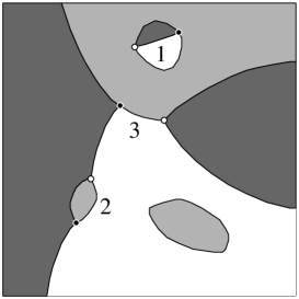
Figure 2: Schematic plot of domain walls of three-state topology showing the three possible vertex types. Black (white) bullets represent vertices (antivertices). The inserted figures denote the number of different antivertices connected to a given vertex.

In order to have a picture about the essence of our topological analysis Fig. 2 illustrates schematically a typical part of the three-color maps on a continuous background if the motion of interfaces is characterized by infinitesimally small steps. In this case we can neglect those vertices were more than three states meet. In such a map the typical objects are the islands and the three-edge vertices. An (isolated) island is surrounded by the same domain therefore its boundary is free of vertices. In fact, two types of vertices (called vertices and antivertices) can be distinguished depending on whether we find 0, 1, 2 or reversed order of states when going around the center in clock-wise direction. The vertices and antivertices are located alternately along the boundaries. Each vertex can be connected to one, two, or three antivertices thus they can be further classified according to the number of linked antivertices. For example, the one-neighbor vertex is represented by a vertex-antivertex pair linked to each other by three edges (see Fig. 2). The concentration of these vertices are denoted by $\rho_{1}$, $\rho_{2}$, or $\rho_{3}$, respectively, and referred as one-, two-, and three-neighbor vertices. The total concentration of vertices is given as $\rho=\rho_{1}+\rho_{2}+\rho_{3}$.

In a previous work Szabó and Szolnoki (2002) we have developed a method to determine the concentration of vertices and also to study some geometrical features (e.g., arclength measured in lattice constant unit) of the vertex edges. Now the capacity of this method is extended by allowing a distinction between the one-, two-, and three-neighbor vertices. Unfortunately, on a square lattice this methods requires the elimination of the four-edge vertices before the geometrical analysis of a given pattern. It is found, however, that this manipulation causes only a minor change (much less than one percent) in the Potts (interfacial) energy except a short transient period. At the same time we can get a more complete picture of the domain growth.

Following an earlier suggestion Tainaka and Itoh (1991) the inverse of vertex concentration can be considered as a rough estimation of the average area of the growing domains that increases linearly with time. The inset of Fig. 3 demonstrates that instead of $\rho$, the concentration of three-neighbor vertices ($\rho_{3}$) gives a much better estimate for the expected linear increase in the averaged domain area for the Potts model. Notice furthermore, that the time dependences of $\rho_{3}^{-1}$ are very similar for the Potts and modified voter models (see Fig. 3) despite the noticeable different behaviors in $\rho_{2}$ and $\rho_{1}$ as discussed below.

Figure 3: The inverse of $\rho_{3}$ as a function of time for the Potts model (filled boxes) and extended voter model (open boxes). The inset shows the inverse of total concentration of vertices $\rho$ (pluses) and the concentration of three-neighbor vertices $\rho_{3}$ (circles) for Potts model. The scales of time and concentration agree with those of the main plot.

The geometrical analysis allows us to determine the time dependence of the total perimeter of isolated islands per sites, $E_{i}$ as a portion of interfacial energy $E(t)$. Since we have monitored the average length of vertex edges ($l_{v}$) during the simulation, the total length of vertex edges per sites can be expressed as $E_{v}=3\rho l_{v}$. Thus the interfacial energy of islands is given as :

$$E_{i}=E(t)-3\rho l_{v}\;.$$ (4)

The simulations indicate strikingly different behaviors in $E_{i}$ for the above three models as plotted in Fig. 4. Surprisingly, $E_{i}$ increases monotonously for the voter model in the time region in which we could study this system. It is expected, however, that $E_{i}$ will decrease for longer times because it is a part of the total interfacial energy vanishing as $1/\ln(t)$ Frachebourg and Krapivsky (1996); Ben-Naim et al. (1996). For the Potts model $E_{i}$ decreases and tends towards a limit value dependent on temperature. This limit value, which is consistent with the corresponding thermal average value of Potts energy ($E_{T}$), comes from the contribution of islands generated by the thermal fluctuations within the large domains. In the third model $E_{i}$ approaches asymptotically to an algebraic decay ($E_{i}\propto t^{-1/2}$) manifesting the surface tension-driven shrink of islands. Notice that here the dynamical rule prohibits the creation of islands inside a homogeneous domain.

Figure 4: The interfacial energies of islands per sites as a function of time. The symbols are the same as in Fig. 1. The solid line has a slope of $-0.5$.

The significant differences in the vertex dynamics can also be perceived when analyzing the $\rho_{1}/\rho$ portion of the one-neighbor vertices. Figure 5 shows that $\rho_{1}/\rho$ (as well as $\rho_{2}/\rho$) tends towards a fixed ratio for the voter model. It can be assumed that the ratio $\rho_{1}:\rho_{2}:\rho_{3}$ remains fixed for larger times too. Conversely, in the Potts model the one-neighbor vertices become dominant for long times because the concentration of the three-neighbor vertices vanishes as $\rho_{3}\propto 1/t$ (see Fig. 3) meanwhile $\rho_{2}\propto 1/\sqrt{t}$ in the asymptotic time regime.

Figure 5: The ratio $\rho_{1}/\rho$ versus time for the three models. Symbols as in Fig. 1.

For the Potts model the appearance of a new state (e.g., state 0) inside a domain (of type 1 or 2) represents the birth of a new island. The occurrence of this island at the boundaries between the domains of type 1 and 2 yields the creation of a three- or two-neighbor vertex-antivertex pair (see Fig. 2). In the third model, however, the extinction of both the one- and two-neighbor vertices as well as of the islands are driven by interfacial energy (as it happens for the Potts model). At the same time their extinction is not compensated by their creation via the appearance of a new type of domain. As a result, the ratio $\rho_{1}/\rho$ and $\rho_{2}/\rho$ tends to zero with the total concentration of vertex in the long time limit.

In the absence of interfacial energy (voter model) the interfaces become more and more irregular Dornic et al. (2001) and the occasional overhanging represents a mechanism to create a new island. These islands move, change their form, and meet randomly. The meeting of two islands of the same type represents their fusion and the contact of two islands of different types creates a three-neighbor vertex-antivertex pair. Similarly, if an island meets a vertex edge then a two-neighbor vertex-antivertex pair is created. All of these and the reversed processes are due to the uncorrelated, random motion of interfaces. The above results suggest the emergence of some fixed ratio between the number of one-, two-, and three-neighbor vertices in the meantime the typical domain size increases logarithmically.

In summary, in the present work we have quantified the topological differences occurring during the two-dimensional domain growth in three-state systems. The analysis is focused on the time-dependence of the concentration of the one-, two-, and three-neighbor vertices as well as on the interfacial energy of islands. The numerical investigations indicate that the concentrations of the three types of vertices tend very slowly towards to fixed ratios while the typical length scale increases as $r\sim\ln t$ in the voter model. In the Potts model the interfacial energy results in a faster domain growth (if $T<T_{c}$) and the vertex dynamics is governed by the appearance of islands and of the one- and two-neighbor vertex-antivertex pairs created by the thermal noise. Above the critical temperature these processes prevent the domain growth. In the extended voter model the introduction of surface tension changes the dynamics of growth dramatically. Similarly to the voter model the domain growth takes place for arbitrary value of temperature but the interfacial energy reduces the creation of islands as well as of the one- and two-neighbor vertices. As a consequence, in this case the growth dynamics becomes equivalent to those characterized by the Allen-Cahn universality class.