Optical properties of unconventional superconductors

Abstract

The optical conductivity measurements give a powerful tool to investigate the nature of the superconducting gap for conventional and unconventional superconductors. In this article, first, general analyses of the optical conductivity are given stemmed from the Mattis-Bardeen formula for conventional BCS superconductors to unconventional anisotropic superconductors. Second, we discuss the reflectance-transmittance (R-T) method which has been proposed to measure far-infrared spectroscopy. The R-T method provides us precise measurements of the frequency-dependent conductivity. Third, the optical conductivity spectra of the electron-doped cuprate superconductor Nd_2-xCe_xCuO₄ are investigated based on the anisotropic pairing model. It is shown that the behavior of optical conductivity is consistent with an anisotropic gap and is well explained by the formula for d-wave pairing in the far-infrared region. The optical properties of the multiband superconductor MgB₂, in which the existence of superconductivity with relatively high-$T_{c}$ (39K) was recently announced, is also examined to determine the symmetry of superconducting gaps.

I Introduction

The measurements of optical properties provide us important insights concerning the nature of charge carries, pseudogaps and superconducting gaps, as well as the electronic band structure of a material.tim89 The optical spectroscopy gives a view into the electronic structure, low-lying excitations, phonon structure, etc. The optical conductivity or the dielectric function indicates a response of a system of electrons to an applied field. For the ordinary superconductors the evidence for an energy gap has been obtained by infrared spectroscopy. Far above the superconducting energy gap, a bulk superconductor behaves like a normal metal in the optical response. The Mattis-Bardeen formula derived in the BCS theory consistently describes the infrared behaviors in the classical conventional superconductors. After the discovery of high-temperature superconductivity, a large amount of works has been made to find the superconducting gap and any spectral features responsible to the superconducting pairing, using an infrared spectroscopy technique.

Optical properties are discussed in the linear response theory where the induced currents are proportional to the external applied field. General formulas have been derived for the optical response. In this paper in Section II we discuss the linear response theory for the conductivity; we derive the Mattis-Bardeen formula for conventional superconductors and the formula for London superconductors. The conductivity sum rule is briefly discussed here.

In Section III we briefly present a new method to characterize far-infrared optical properties which we call the reflectance-transmittance method (R-T method). In this method, both the reflectance spectra $R(\omega)$ and the transmittance spectra $T(\omega)$ are measured, and then they are substituted into a set of coupled equations which describe exactly the transmittance and reflectance of thin films. The coupled equations are solved numerically by the Newton method to obtain the complex refractive indices $n$ and $k$ of thin films as functions of the frequency $\omega$, which determined the optical conductivity $\sigma(\omega)$. Since this method does not need a Kramers-Kronig transformation, we are free from difficulties stemmed from uncertainties in the small $\omega$ region in the conventional method.

In the subsequent Sections we discuss two materials: the electron-doped oxide superconductor Nd_2-xCe_xCuO₄ and the magnesium diboride MgB₂ exhibiting $T_{c}=39$K. The cuprate high-$T_{c}$ superconductors are regarded as a typical London superconductor satisfying $\lambda\gg\xi$ for the penetration depth and the coherence length. Our date obtained from the R-T method for Nd_2-xCe_xCuO₄ clearly indicates the $d$-wave symmetry with nodes for the superconducting gap.

MgB₂ is recently discovered superconductor with a relatively high $T_{c}$ in spite of its simple crystal structure. The symmetry of Cooper pairs is an issue which should be clarified to investigate the mechanism of high $T_{c}$. The optical properties provide us information on superconducting gaps from which we conclude that this material is described by two order parameters attached to $\sigma$- and $\pi$-bands. Besides, the two order parameters have different anisotropy to explain the experimental results consistently.

II Theory of Optical Conductivity

II.1 Linear Response Theory

In this section we discuss the optical properties in the linear response theory in the normal metal and superconductors. The famous Mattis-Bardeen formula is derived and its modifications to unconventional superconductors are discussed. In the Kubo theory the external applied field

$$H^{\prime}(t)=-\sum_{\mu}a_{\mu}X_{\mu}(t)=-\sum_{\mu}a_{\mu}X_{\mu}{\rm e}^{-i\omega t},$$ (1)

is considered as a perturbation to the non-interacting system described by the Hamiltonian $H_{0}$. The total Hamiltonian is given by $H=H_{0}+H^{\prime}$. From the equation $i\hbar\partial\rho/\partial t=[H,\rho]$, a linear variation $\rho^{\prime}(t)$ to the density operator $\rho_{0}={\rm e}^{-\beta H_{0}}/Z_{0}$ is written as

$$i\hbar\frac{\partial\rho^{\prime}}{\partial t}=[H_{0},\rho^{\prime}]+[H^{\prime},\rho_{0}].$$ (2)

Then $\rho^{\prime}$ is given as

$$\rho^{\prime}(t)=-\frac{i}{\hbar}\int^{t}_{-\infty}dt^{\prime}{\rm e}^{-iH_{0}(t-t^{\prime})/\hbar}[H^{\prime}(t^{\prime}),\rho_{0}]{\rm e}^{iH(t-t^{\prime})/\hbar}.$$ (3)

For the electrical conductivity, the external fields are given by

$$a_{\mu}=e\sum_{i}x_{i\mu},~{}~{}X_{\mu}=E_{\mu}~{}~{}(\mu=x,y,z).$$ (4)

The current is given by

$$J_{\mu}=\dot{a}_{\mu}=e\sum_{i}(\dot{x}_{i})_{\mu}=e\sum_{i}(v_{i})_{\mu}.$$ (5)

The expectation value of the current is

$$\langle J_{\mu}(t)\rangle = {\rm Tr}\rho^{\prime}J_{\mu}$$ (6)

$$= -\frac{i}{\hbar}\int^{t}_{-\infty}dt^{\prime}{\rm Tr}{\rm e}^{-iH_{0}(t-t^{\prime})/\hbar}[H^{\prime}(t^{\prime}),\rho_{0}]{\rm e}^{iH_{0}(t-t^{\prime})/\hbar}J_{\mu}$$

$$= \frac{i}{\hbar}\int^{\infty}_{0}d\tau{\rm e}^{i\omega\tau}{\rm Tr}{\rm e}^{-iH_{0}\tau/\hbar}[a_{\nu},\rho_{0}]{\rm e}^{iH_{0}\tau/\hbar}E_{\nu}{\rm e}^{-i\omega t}J_{\mu}.$$

We assume the time dependence of $\langle J_{\mu}(t)\rangle$ as $\langle J_{\mu}(t)\rangle=J_{\mu}(\omega){\rm e}^{-i\omega t}$, then we obtain

$$J_{\mu}(\omega)=\sigma_{\mu\nu}(\omega)E_{\nu},$$ (7)

where the conductivity is written as

$$\sigma_{\mu\nu}(\omega) = \frac{i}{\hbar}\int^{\infty}_{0}dt{\rm e}^{i\omega t}{\rm Tr}{\rm e}^{-iH_{0}t/\hbar}[a_{\nu},\rho_{0}]{\rm e}^{iH_{0}t/\hbar}J_{\mu}$$ (8)

$$= \int^{\infty}_{0}dt{\rm e}^{i\omega t}\phi_{\mu\nu}(t).$$

Here we have defined

$$\phi_{\mu\nu}(t)=\frac{i}{\hbar}{\rm Tr}[a_{\nu},\rho_{0}]{\rm e}^{iH_{0}t/\hbar}J_{\mu}{\rm e}^{-iH_{0}t/\hbar}.$$ (9)

Due to the relation

$$[a_{\nu},\rho_{0}]=-i\hbar\rho_{0}\int^{\beta}_{0}d\lambda\dot{a}_{\nu}(-i\hbar\lambda),$$ (10)

we obtain

$$\phi_{\mu\nu}(t) =\int^{\beta}_{0}d\lambda{\rm Tr}\rho_{0}\dot{a}_{\nu}(-i\hbar\lambda)J_{\mu}(t)$$ (11)

$$=\int^{\beta}_{0}d\lambda\langle J_{\nu}(-i\hbar\lambda)J_{\mu}(t)\rangle.$$

Since the time-derivative of $\phi$ is written as

$$\dot{\phi}_{\mu\nu}=-\frac{i}{\hbar}\langle J_{\mu}(t)J_{\nu}(0)-J_{\nu}(0)J_{\mu}(t)\rangle,$$ (12)

the conductivity is given by

$$\sigma_{\mu\nu}(\omega) = \int^{\infty}_{0}{\rm e}^{i\omega t}\phi_{\mu\nu}(t)=-\int^{\infty}_{0}dt\frac{{\rm e}^{i(\omega+i\delta)t}-1}{i(\omega+i\delta)}\dot{\phi}_{\mu\nu}$$ (13)

$$= -\int^{\infty}_{-\infty}dt\frac{{\rm e}^{i(\omega+i\delta)t}-1}{i(\omega+i\delta)}Q^{R}_{\mu\nu}(t)$$

$$= -\frac{1}{i(\omega+i\delta)}[Q^{R}_{\mu\nu}(\omega)-Q^{R}_{\mu\nu}(0)],$$

where

$$Q^{R}_{\mu\nu}(t)=-\frac{i}{\hbar}\theta(t)\langle[J_{\mu}(t),J_{\nu}(0)]\rangle,$$ (14)

and $Q^{R}_{\mu\nu}(\omega)$ is its Fourier transform. $Q^{R}_{\mu\nu}(\omega)$ is evaluated from the analytic continuation of the thermal Green’s function:

$$Q^{R}_{\mu\nu}(\omega)=Q_{\mu\nu}(i\omega_{n}\rightarrow\hbar\omega+i\delta),$$ (15)

$$Q_{\mu\nu}(\tau)=-\langle{\rm T}J_{\mu}(\tau)J_{\nu}(0)\rangle=\frac{1}{\beta}\sum_{\omega_{n}}Q_{\mu\nu}(i\omega_{n}){\rm e}^{-i\omega_{n}\tau}.$$ (16)

From these equations we can derive the sum rule for $\sigma_{\mu\nu}$. Let us define the Fourier transform of $\phi_{\mu\nu}(t)$ as

$$\phi_{\mu\nu}(\omega)=\int^{\infty}_{-\infty}dt\phi_{\mu\nu}(t){\rm e}^{i\omega t},$$ (17)

then $\sigma_{\mu\nu}(\omega)$ is written as

$$\sigma_{\mu\nu}(\omega)=\frac{i}{2\pi}\int^{\infty}_{-\infty}d\omega^{\prime}\phi_{\mu\nu}(\omega^{\prime})\frac{1}{\omega-\omega^{\prime}+i\delta}.$$ (18)

Hence the following formulae are followed:

$$\int^{\infty}_{-\infty}d\omega\sigma_{\mu\nu}(\omega)=\pi\phi_{\mu\nu}(t=0),$$ (19)

$$\lim_{\omega\rightarrow 0}\omega\sigma_{\mu\nu}(\omega)=i\phi_{\mu\nu}(t=0).$$ (20)

Since $v_{i\mu}=(1/m)(p_{i\mu}-(e/c)A_{\mu})$ and $J_{\mu}=e\sum_{i}(v_{i})_{\mu}$, we obtain

$$\phi_{\mu\nu}(t=0) = \frac{i}{\hbar}{\rm Tr}[a_{\nu},\rho_{0}]J_{\mu}$$ (21)

$$= \frac{i}{\hbar}{\rm Tr}(\rho_{0}[J_{\mu},\sum_{j}ex_{j\nu}])$$

$$= \delta_{\mu\nu}\frac{Ne^{2}}{m}.$$

Then the sum rule is written as

$$\int^{\infty}_{0}d\omega{\rm Re}\sigma(\omega)=\frac{\pi}{2}\frac{Ne^{2}}{m}$$ (22)

In this derivation the translational invariance of the potential term is important since we used the relation $\dot{x}_{i\mu}=v_{i\mu}=(1/m)(p_{i\mu}-(e/c)A_{\mu})$. In the Drude formula

$$\sigma(\omega)=\frac{Ne^{2}}{m}\frac{\tau}{1-i\omega\tau},$$ (23)

the sum rule is clearly satisfied.

Please note that the above formulas are derived for the uniform external fields. An extension to the spatially oscillating fields is performed in a straightforward way. Here we set $\hbar=1$. Let us consider the spatially varying applied fields:

$$H^{\prime}(t)=-\frac{1}{c}\int d{\bf r}\xi_{\mu}({\bf r})E_{\mu}({\bf r},t),$$ (24)

or

$$H^{\prime}(t)=-\frac{1}{c}\int d{\bf r}j_{\mu}({\bf r})A_{\mu}({\bf r},t),$$ (25)

where we assume

$$E_{\mu}({\bf r},t)=e_{\mu}{\rm e}^{i({\bf q}\cdot{\bf r}-\omega t)},$$ (26)

and $A_{\mu}({\bf r},t)$ is the vector potential satisfying $E_{\mu}({\bf r},t)=(-1/c)\dot{A}_{\mu}({\bf r},t)=(i\omega/c)A_{\mu}({\bf r},t)$ and ${\rm div}{\bf A}=0$. We set $\xi_{\mu}({\bf r},t)=e\sum_{i}x_{i\mu}\delta({\bf r}-{\bf r}_{i})$ and $j_{\mu}$ is the current operator given by

$$j_{\mu}({\bf r})=\frac{1}{2m}\sum_{i}e[{\bf p}_{i}\delta({\bf r}-{\bf r}_{i})+\delta({\bf r}-{\bf r}_{i}){\bf p}_{i}]_{\mu}.$$ (27)

The conductivity is defined as the coefficient of the linear response of the current to applied fields:

$$J_{\mu}({\bf r},t) = \sigma_{\mu\nu}({\bf q},\omega)E_{\nu}({\bf r},t)$$ (28)

$$= \int d{\bf r}^{\prime}\int^{t}_{-\infty}dt^{\prime}\sigma_{\mu\nu}({\bf r}-{\bf r}^{\prime};t-t^{\prime})E_{\nu}({\bf r}^{\prime},t^{\prime}).$$

The expectation value of $j_{\mu}({\bf r})$ to the first order in $H^{\prime}$ is evaluated as

$$\langle j_{\mu}({\bf r},t)\rangle = {\rm Tr}\rho^{\prime}j_{\mu}({\bf r})$$ (29)

$$= i\int^{\infty}_{0}dt^{\prime}\int d{\bf r}{\rm Tr}{\rm e}^{-iH_{0}t^{\prime}}[\xi_{\nu}({\bf r}),\rho_{0}]{\rm e}^{iH_{0}t^{\prime}}e_{\nu}{\rm e}^{i{\bf q}\cdot{\bf r}}{\rm e}^{-i\omega(t-t^{\prime})}j_{\mu}({\bf r})$$

$$= \frac{i}{\hbar}\int^{\infty}_{0}dt^{\prime}{\rm e}^{i\omega t^{\prime}}{\rm Tr}{\rm e}^{-iH_{0}t^{\prime}}[\xi_{\nu}({\bf q}),\rho_{0}]{\rm e}^{iH_{0}t^{\prime}}e_{\nu}{\rm e}^{-i\omega t}j_{\mu}({\bf r}),$$

where $\xi_{\mu}({\bf q})$ is the Fourier transform of $\xi_{\mu}({\bf r})$. We follow the same procedure as for the uniform external fields and note that $\dot{\xi}_{\mu}({\bf r})=J_{\mu}({\bf r})$, then we have

$$\phi_{\mu\nu}({\bf q},t)=\int^{\beta}_{0}d\lambda\langle j_{\nu}({\bf q},-i\hbar\lambda)j_{\mu}({\bf r},t)\rangle{\rm e}^{-i{\bf q}\cdot{\bf r}}.$$ (30)

Here we neglect the ${\bf A}$-term in the current $J_{\mu}$ since this is the higher-order term in external fields and we take a spatial average to write

$$j_{\mu}({\bf q})=\int d{\bf r}j_{\mu}({\bf r}){\rm e}^{i{\bf q}\cdot{\bf r}}=\frac{e}{2m}\sum_{i}({\bf p}_{i}{\rm e}^{i{\bf q}\cdot{\bf r}_{i}}+{\rm e}^{i{\bf q}\cdot{\bf r}_{i}}{\bf p}_{i})_{\mu},$$ (31)

$$\phi_{\mu\nu}({\bf q},t)=\int^{\beta}_{0}d\lambda\langle j_{\nu}({\bf q},-i\hbar\lambda)j_{\mu}({\bf q},t)\rangle,$$ (32)

$$\sigma_{\mu\nu}({\bf q},\omega)=\int^{\infty}_{0}dt{\rm e}^{i\omega t}\phi_{\mu\nu}({\bf q},t).$$ (33)

Now let us define the retarded response function:

$$K_{\mu\nu}({\bf q},t-t^{\prime})=-i\theta(t-t^{\prime})\langle[j_{\mu}^{{\dagger}}({\bf q},t),j_{\nu}({\bf q},t^{\prime})]\rangle,$$ (34)

and its Fourier transform given by

$$K_{\mu\nu}({\bf q},\omega)=\int^{\infty}_{-\infty}dt{\rm e}^{i\omega t}K_{\mu\nu}({\bf q},t).$$ (35)

The formula for the optical conductivity is followed as

$$\sigma_{\mu\nu}({\bf q},\omega)=\frac{i}{\omega+i\delta}[K_{\mu\nu}({\bf q},\omega)-K_{\mu\nu}({\bf q},0)].$$ (36)

The current response function is written in the form,

$$K_{\mu\nu}({\bf q},\omega+i\delta)=-\sum_{nm}\frac{{\rm e}^{-\beta E_{n}}}{Z}[\frac{\langle n|j_{\nu}({\bf q})|m\rangle\langle m|j^{{\dagger}}_{\mu}({\bf q})|n\rangle}{E_{m}-E_{n}+\omega+i\delta}-\frac{\langle n|j^{{\dagger}}_{\mu}({\bf q})|m\rangle\langle m|j_{\nu}({\bf q})|n\rangle}{E_{n}-E_{m}+\omega+i\delta}],$$ (37)

where $|n\rangle$ denotes a complete set of exact eigenstates of $H_{0}$ with eigenvalues $E_{n}$ and $Z$ is the partition function $Z=\sum_{n}{\rm e}^{-\beta E_{n}}$. The imaginary part of $K_{\mu\nu}$ is given by

$${\rm Im}K_{\mu\nu}({\bf q},\omega+i\delta)=-\pi(1-{\rm e}^{-\beta\omega})\sum_{nm}\frac{{\rm e}^{-\beta E_{n}}}{Z}\delta(E_{m}-E_{n}-\omega)\langle n|j^{{\dagger}}_{\mu}({\bf q})|m\rangle\langle m|j_{\nu}({\bf q})|n\rangle.$$ (38)

The retarded Green’s function $K_{\mu\nu}({\bf q},\omega)$ is evaluated from the thermal Green’s function through the analytic continuation:

$$K_{\mu\nu}({\bf q},\omega)=K_{\mu\nu}({\bf q},i\omega_{n}=\omega+i\delta),$$ (39)

where

$$K_{\mu\nu}({\bf q},i\omega_{n})=\int^{\beta}_{0}d\tau{\rm e}^{i\omega_{n}\tau}K_{\mu\nu}({\bf q},\tau),$$ (40)

$$K_{\mu\nu}({\bf q},\tau)=-\langle Tj^{{\dagger}}_{\mu}({\bf q},\tau)j_{\nu}({\bf q},0)\rangle.$$ (41)

In order to calculate the conductivity for the uniform external fields, we take the limit ${\bf q}\rightarrow 0$. For the direct-current conductivity, we must take the limit ${\bf q}\rightarrow 0$ first before $\omega\rightarrow 0$. The current operator is given by

$${\bf j}({\bf q})=\frac{e}{m}\sum_{{\bf p}\sigma}({\bf p}+\frac{1}{2}{\bf q})c^{{\dagger}}_{{\bf p}+{\bf q}\sigma}c_{{\bf p}\sigma}=\frac{e}{m}\sum_{{\bf p}\sigma}{\bf p}c^{{\dagger}}_{{\bf p}+{\bf q}/2,\sigma}c_{{\bf p}-{\bf q}/2,\sigma}.$$ (42)

In the limit ${\bf q}\rightarrow 0$ $K_{\mu\nu}({\bf q},\omega=0)$ is evaluated as

$$K_{\mu\nu}(0,0) = \frac{2e^{2}}{m^{2}}\frac{1}{\beta}\sum_{n}\sum_{{\bf k}}k_{\mu}k_{\nu}G_{0}({\bf k},i\epsilon_{n})^{2}$$ (43)

$$= \frac{2e^{2}}{m^{2}}\frac{1}{\beta}\sum_{n}\sum_{\bf k}k_{\mu}\frac{m}{2}\frac{\partial}{\partial k_{\nu}}G_{0}({\bf k},i\epsilon_{n})=\frac{2e^{2}}{m^{2}}\frac{m}{2}\frac{1}{\beta}\sum_{n}\sum_{\bf k}(-\delta_{\mu\nu})G_{0}({\bf k},i\epsilon_{n})$$

$$= -\frac{Ne^{2}}{m}\delta_{\mu\nu},$$

where $G_{0}({\bf k},i\epsilon_{n})$ is the Green’s function for the non-interacting electrons: $G_{0}({\bf k},i\epsilon_{n})=(i\epsilon_{n}-\epsilon_{{\bf k}})^{-1}$ for $\epsilon_{n}=(2n+1)\pi/\beta$. Then the uniform conductivity is given by the formula

$$\sigma_{\mu\nu}(\omega)=\frac{i}{\omega+i\delta}[K_{\mu\nu}({\bf q}=0,\omega+i\delta)+\frac{Ne^{2}}{m}\delta_{\mu\nu}].$$ (44)

The current response function $K_{\mu\nu}$ for ${\bf q}\neq 0$ in the non-intracting system is

$$K_{\mu\nu}({\bf q},i\omega_{n})=-\frac{2e^{2}}{m^{2}}\sum_{\bf p}p_{\mu}p_{\nu}\frac{f(\epsilon_{{\bf p}-{\bf q}/2})-f(\epsilon_{{\bf p}+{\bf q}/2})}{-i\omega_{n}+\epsilon_{{\bf p}-{\bf q}/2}-\epsilon_{{\bf p}+{\bf q}/2}}.$$ (45)

Since $K_{\mu\nu}({\bf q},\omega)$ vanishes in the limit ${\bf q}\rightarrow 0$ for finite $\omega\neq 0$, we have the sum rule

$$\int^{\infty}_{0}d\omega{\rm Re}\sigma_{\mu\nu}(\omega)=\frac{\pi}{2}\frac{Ne^{2}}{m}\delta_{\mu\nu},$$ (46)

and the Drude weight

$$D=\frac{\pi Ne^{2}}{m}$$ (47)

as the coefficient of the delta function: Re$\sigma_{\mu\nu}(\omega)=D\delta(\omega)\delta_{\mu\nu}$. The sum rule for ${\bf q}\neq 0$ is derived similarly. The commutator $[j^{{\dagger}}_{\mu},\xi_{\nu}]$ as in eq.(21) leads to

$$\int^{\infty}_{-\infty}d\omega{\rm Re}\sigma_{\mu\nu}({\bf q},\omega)=\pi{\rm Re}\phi_{\mu\nu}({\bf q},t=0)=\frac{\pi Ne^{2}}{m}\delta_{\mu\nu}.$$ (48)

II.2 Mattis-Bardeen Formula

The infrared absorption formula in BCS model was first derived by Mattis-Bardeen.mat58 We use the standard notations for the Green’s functions;

$$G({\bf p},\tau)=-\langle c_{{\bf p}\sigma}(\tau)c^{{\dagger}}_{{\bf p}\sigma}(0)\rangle,$$ (49)

$$F({\bf p},\tau)=\langle c_{-{\bf p}\downarrow}(\tau)c_{{\bf p}\uparrow}(0)\rangle,$$ (50)

$$F^{{\dagger}}({\bf p},\tau)=\langle c^{{\dagger}}_{{\bf p}\uparrow}(\tau)c^{{\dagger}}_{-{\bf p}\downarrow}(0)\rangle,$$ (51)

and their Fourier transforms given by

$$G({\bf p},i\epsilon_{n})=\frac{u^{2}_{{\bf p}}}{i\epsilon_{n}-E_{{\bf p}}}+\frac{v^{2}_{{\bf p}}}{i\epsilon_{n}+E_{{\bf p}}},$$ (52)

$$F({\bf p},i\epsilon_{n})=F^{{\dagger}}({\bf p},i\epsilon_{n})=-u_{{\bf p}}v_{{\bf p}}(\frac{1}{i\epsilon_{n}-E_{{\bf p}}}-\frac{1}{i\epsilon_{n}+E_{{\bf p}}}),$$ (53)

where $E_{{\bf p}}=\sqrt{\xi_{{\bf p}}^{2}+\Delta^{2}_{{\bf p}}}$, $u^{2}_{{\bf p}}=(1/2)(1+\xi_{{\bf p}}/E_{{\bf p}})$ and $v^{2}_{{\bf p}}=1-u^{2}_{{\bf p}}$ for $\xi_{{\bf p}}=\epsilon_{{\bf p}}-\mu$. We evaluate the current response function written as

$$K_{\mu\nu}({\bf q},i\omega_{\ell}) = \frac{2e^{2}}{m^{2}}\sum_{{\bf p}}p_{\mu}p_{\nu}\frac{1}{\beta}\sum_{n}[G({\bf p}-{\bf q}/2,i\epsilon_{n})G({\bf p}+{\bf q}/2,i\epsilon_{n}-i\omega_{\ell})$$ (54)

$$+ F({\bf p}-{\bf q}/2,i\epsilon_{n})F^{{\dagger}}({\bf p}+{\bf q}/2,i\epsilon_{n}+i\omega_{\ell})].$$

We set $i\omega_{\ell}\rightarrow-i\omega_{\ell}$ in the first term, then using the symmetry ${\bf q}\leftrightarrow-{\bf q}$ we have

$$K_{\mu\nu}({\bf q},i\omega_{\ell}) = \frac{2e^{2}}{m^{2}}\sum_{{\bf p}}p_{\mu}p_{\nu}[(f(E_{{\bf p}_{+}})-f(E_{{\bf p}_{-}}))\frac{1}{2}\left(1+\frac{\xi_{{\bf p}_{+}}\xi_{{\bf p}_{-}}}{E_{{\bf p}_{+}}E_{{\bf p}_{-}}}+\frac{\Delta_{{\bf p}_{+}}\Delta_{{\bf p}_{-}}}{E_{{\bf p}_{+}}E_{{\bf p}_{-}}}\right)\frac{1}{i\omega_{\ell}+E_{{\bf p}_{+}}-E_{{\bf p}_{-}}}$$

$$+ (f(E_{{\bf p}_{+}})+f(E_{{\bf p}_{-}})-1)\frac{1}{4}\left((1+\frac{\xi_{{\bf p}_{+}}}{E_{{\bf p}_{+}}})(1-\frac{\xi_{{\bf p}_{-}}}{E_{{\bf p}_{-}}})-\frac{\Delta_{{\bf p}_{+}}\Delta_{{\bf p}_{-}}}{E_{{\bf p}_{+}}E_{{\bf p}_{+}}}\right)\frac{1}{i\omega_{\ell}+E_{{\bf p}_{+}}+E_{{\bf p}_{-}}}$$

$$+ (1-f(E_{{\bf p}_{+}})-f(E_{{\bf p}_{-}}))\frac{1}{4}\{(1-\frac{\xi_{{\bf p}_{+}}}{E_{{\bf p}_{+}}})(1+\frac{\xi_{{\bf p}_{-}}}{E_{{\bf p}_{-}}})-\frac{\Delta_{{\bf p}_{+}}\Delta_{{\bf p}_{-}}}{E_{{\bf p}_{+}}E_{{\bf p}_{+}}}\}\frac{1}{i\omega_{\ell}-E_{{\bf p}_{+}}-E_{{\bf p}_{-}}}],$$

where ${\bf p}_{+}={\bf p}+{\bf q}/2$ and ${\bf p}_{-}={\bf p}-{\bf q}/2$. Here we consider (i) dirty superconductors or (ii) thin films satisfying $d\ll\xi\approx v_{F}/\Delta$ for the film thickness $d$ and the coherence length $\xi$. In these cases we can regard ${\bf p}_{+}$ and ${\bf p}_{-}$ as independent variables. In the case (ii), since $qv_{F}\gg\Delta\sim\omega$ we can do Abrikosov’s replacementabr88 ,

$$\sum_{{\bf p}}\rightarrow N(0)\frac{1}{4qv_{F}}\int d\xi_{{\bf p}_{+}}d\xi_{{\bf p}_{-}}.$$ (56)

Then in the isotropic case we obtain the Mattis-Bardeen formulae for $\sigma_{1}(\omega)={\rm Re}\sigma(\omega)=-(1/\omega){\rm Im}K(\omega+i\delta)$ and $\sigma_{2}(\omega)={\rm Im}\sigma(\omega)=(1/\omega){\rm Re}K(\omega+i\delta)$:

$$\frac{\sigma_{1s}}{\sigma_{1n}}(\omega) = \frac{1}{\omega}\int^{\omega-\Delta}_{\Delta}dEN(E)N(\omega-E)(1-2f(\omega+E))\left(1-\frac{\Delta^{2}}{E(\omega-E)}\right)\theta(\omega-2\Delta)$$ (57)

$$+ 2\frac{1}{\omega}\int^{\infty}_{0}dE(f(E)-f(\omega+E))\left(1+\frac{\Delta^{2}}{E(\omega+E)}\right),$$

$$\frac{\sigma_{2s}}{\sigma_{1n}}(\omega)=\frac{1}{\omega}\int^{\Delta}_{max(-\Delta,\Delta-\omega)}dE(1-2f(\omega+E))\frac{E(E+\omega)+\Delta^{2}}{\sqrt{\Delta^{2}-E^{2}}\sqrt{(E+\omega)^{2}-\Delta^{2}}},$$ (58)

where $\sigma_{1n}$ is the real part of the conductivity for normal state. In the above formula for $\sigma_{2}$, the integral is calculated as follows.

$$I \equiv \frac{1}{4}\int^{\infty}_{-\infty}d\xi_{p}d\xi_{p^{\prime}}(1-\frac{\xi_{p}\xi_{p^{\prime}}+\Delta^{2}}{E_{p}E_{p^{\prime}}}){\rm P}\frac{1}{\omega-E_{p}-E_{p^{\prime}}}$$ (59)

$$= \int^{\infty}_{\Delta}dEdE^{\prime}N(E)N(E^{\prime})(1-\frac{\Delta^{2}}{EE^{\prime}}){\rm P}\frac{1}{\omega-E_{p}-E_{p^{\prime}}}$$

$$= \int^{\infty}_{-\infty}d\epsilon\int^{\infty}_{\Delta}dEdE^{\prime}N(E)N(E^{\prime})(1-\frac{\Delta^{2}}{EE^{\prime}}){\rm P}\frac{1}{\omega-\epsilon}\delta(\epsilon+E-E^{\prime})$$

$$= \int^{\infty}_{\Delta-E}d\epsilon\int^{\infty}_{\Delta}dEN(E)N(E+\epsilon)(1-\frac{\Delta^{2}}{E(E+\epsilon)}){\rm P}\frac{1}{\omega-\epsilon}$$

$$= {\rm Re}\int^{\infty}_{-\infty}d\epsilon\int^{\infty}_{\Delta}dEN(E)N(E+\epsilon)(1-\frac{\Delta^{2}}{E(E+\epsilon)})\frac{-1}{2}(\frac{1}{\epsilon+\omega+i\delta}+\frac{1}{\epsilon+\omega-i\delta})$$

$$= \pi{\rm Im}\int^{\infty}_{\Delta}dEN(E)N(E-\omega)(1-\frac{\Delta^{2}}{E(E-\omega)})$$

$$= -\pi\int^{\omega+\Delta}_{max(\omega-\Delta,\Delta)}dE\frac{E(\omega-E)-\Delta^{2}}{\sqrt{E^{2}-\Delta^{2}}\sqrt{\Delta^{2}-(\omega-E)^{2}}}$$

$$= \pi\int^{\Delta}_{max(\Delta-\omega,-\Delta)}dE\frac{E(\omega+E)+\Delta^{2}}{\sqrt{\Delta^{2}-E^{2}}\sqrt{(\omega-E)^{2}-\Delta^{2}}}.$$

At $T=0$, the integral has the form for complete elliptic integrals by changing variables of integration to $x$ where $x=(2E-\omega)/(\omega-2\Delta)$ for $\sigma_{1s}$;

$$\frac{\sigma_{1s}}{\sigma_{1n}}(\omega) = \frac{1}{\omega}\int_{\Delta}^{\omega-\Delta}dE\frac{E(\omega-E)-\Delta^{2}}{\sqrt{E^{2}-\Delta^{2}}\sqrt{(\omega-E)^{2}-\Delta^{2}}}$$ (60)

$$= \frac{\omega-2\Delta}{\omega}\int_{0}^{1}dx\frac{1-kx^{2}}{\sqrt{(1-x^{2})(1-k^{2}x^{2})}},$$

where $k=(\omega-2\Delta)/(\omega+2\Delta)$ and $\omega>2\Delta$. We then obtain the Mattis-Bardeen formula:

$$\frac{\sigma_{1s}}{\sigma_{1n}}(\omega)=\left(\left(1+\frac{2\Delta}{\omega}\right)E(k)-\frac{4\Delta}{\omega}K(k)\right)\theta(\omega-2\Delta),$$ (61)

where

$$E(k)=\int_{0}^{1}\sqrt{\frac{1-k^{2}x^{2}}{1-x^{2}}}dx,~{}~{}K(k)=\int_{0}^{1}\frac{1}{\sqrt{(1-x^{2})(1-k^{2}x^{2})}}dx,$$ (62)

are complete elliptic integrals. An expression for $\sigma_{2s}$ valid for all $\omega$ is

$$\frac{\sigma_{2s}}{\sigma_{1n}}(\omega)=\left(\frac{\Delta}{\omega}+\frac{1}{2}\right)E(k^{\prime})+\left(\frac{\Delta}{\omega}-\frac{1}{2}\right)K(k^{\prime}),$$ (63)

where $k^{\prime}=(1-k^{2})^{1/2}$.

In evaluations of $K_{\mu\nu}$, the matrix notations are also employed for Green’s functions in superconductors,

$$\hat{G}({\bf k},i\epsilon_{n})=\frac{i\tilde{\epsilon_{n}}\tau_{0}+\xi_{{\bf k}}\tau_{3}+\tilde{\Delta}_{{\bf k}}\tau_{1}}{\tilde{\epsilon_{n}}^{2}+\xi_{{\bf k}}^{2}+\tilde{\Delta_{{\bf k}}}^{2}},$$ (64)

where $\tau_{i}$ ($i=0,1,3$) are Pauli matrices. $\epsilon_{n}$ and $\Delta_{{\bf k}}$ are generalized to include the self-energy in the form: $\tilde{\epsilon_{n}}=\epsilon_{n}-\Sigma_{0}(\epsilon_{n})$ and $\tilde{\Delta_{{\bf k}}}=\Delta_{{\bf k}}+\Sigma_{1}(\epsilon_{n})$. The response function $K_{\mu\nu}$ is written as neglecting pair vertex corrections

$$K_{\mu\nu}({\bf q},i\omega_{m})=\frac{e^{2}}{m^{2}}\sum_{{\bf p}}p_{\mu}p_{\nu}\frac{1}{\beta}\sum_{n}{\rm Tr}\hat{G}({\bf p}_{+},i\epsilon_{n}+i\omega_{m})\hat{G}({\bf p}_{-},i\epsilon_{n}).$$ (65)

One can reproduce the Mattis-Bardeen formulae from this expression in a straightforward way.

II.3 Optical Conductivity in London Superconductor

In this section, we investigate the superconductor in the London limit: $\xi\ll\lambda$ for the coherence length $\xi$ and the penetration depth $\lambda$. Since $q\xi\ll 1$ holds, we must consider the limit $q\rightarrow 0$ for the response function in eq.(65)ska64 ; hir89 ; hir92 ; hir94 ; dor00 ; dor03 :

$$K_{\mu\nu}({\bf q},i\omega_{m})=\frac{e^{2}k_{F}^{2}}{m^{2}}2\sum_{{\bf k}}\hat{k}_{\mu}\hat{k}_{\nu}\frac{1}{\beta}\sum_{n}\frac{-\tilde{\epsilon}_{n}(\tilde{\epsilon}_{n}+\omega_{m})+\xi_{{\bf k}_{-}}\xi_{{\bf k}_{+}}+\tilde{\Delta}_{{\bf k}_{-}}\tilde{\Delta}_{{\bf k}_{+}}}{(\tilde{\epsilon}_{n}^{2}+\xi^{2}_{{\bf k}_{-}}+\tilde{\Delta}^{2}_{{\bf k}_{-}})((\tilde{\epsilon}_{n}+\omega_{m})^{2}+\xi^{2}_{{\bf k}_{+}}+\tilde{\Delta}^{2}_{{\bf k}_{+}})}.$$ (66)

We use the notation $\tilde{z}=i\tilde{\epsilon}_{n}=i\epsilon_{n}-i\Sigma_{0}(i\epsilon_{n})=z-i\Sigma_{0}(z)$. Then we have

$$K_{\mu\nu}({\bf q}=0,i\omega_{m})=\frac{e^{2}k_{F}^{2}}{m^{2}}2\sum_{{\bf k}}\hat{k}_{\mu}\hat{k}_{\nu}\frac{1}{2\pi i}\int_{C}dzf(z)\frac{\tilde{z}(\tilde{z}+i\omega_{m})+\xi^{2}_{{\bf k}}+\tilde{\Delta}_{{\bf k}}\tilde{\Delta}_{{\bf k}_{+}}}{(\xi^{2}_{{\bf k}}+\tilde{\Delta}^{2}_{{\bf k}}-\tilde{z}^{2})(\xi^{2}_{{\bf k}}+\tilde{\Delta}^{2}_{{\bf k}_{+}}-(\tilde{z}+i\omega_{m})^{2})},$$ (67)

where $\tilde{\Delta}^{2}_{{\bf k}_{+}}=\Delta+\Sigma_{1}(z+i\omega)$ and $C$ is the contour surrounding the poles of $f(z)$ in the clockwise direction. We set $z_{+}=z+i\omega_{m}$, and write the integrand in the form,

$$\frac{\tilde{z}\tilde{z}_{+}+\xi^{2}_{{\bf k}}+\tilde{\Delta}^{2}_{{\bf k}}\tilde{\Delta}^{2}_{{\bf k}_{+}}}{(\xi^{2}_{{\bf k}}+\tilde{\Delta}^{2}_{{\bf k}}-\tilde{z}^{2})(\xi^{2}_{{\bf k}}+\tilde{\Delta}^{2}_{{\bf k}_{+}}-(\tilde{z}+i\omega_{m})^{2})} = \frac{1}{\xi^{2}_{{\bf k}}+\tilde{\Delta}^{2}_{{\bf k}}-\tilde{z}^{2}}$$

$$+ \frac{\tilde{z}\tilde{z}_{+}+\tilde{\Delta}^{2}_{{\bf k}}\tilde{\Delta}^{2}_{{\bf k}_{+}}+\tilde{z}^{2}_{+}-\tilde{\Delta}^{2}_{{\bf k}_{+}}}{(\xi^{2}_{{\bf k}}+\tilde{\Delta}^{2}_{{\bf k}}-\tilde{z}^{2})(\xi^{2}_{{\bf k}}+\tilde{\Delta}^{2}_{{\bf k}_{+}}-(\tilde{z}+i\omega_{m})^{2})}.$$

Then the momentum summations are performed in the following way:

$$\sum_{{\bf k}}\frac{1}{2\pi i}\int_{C}dzf(z)\frac{1}{\xi^{2}_{{\bf k}}+\tilde{\Delta}^{2}_{{\bf k}}-\tilde{z}^{2}} = N(0)\langle\int_{-\infty}^{\infty}d\xi\frac{1}{2\pi i}\int_{C}dzf(z)\frac{z}{(\xi^{2}+\tilde{\Delta}^{2}_{{\bf k}}-\tilde{z}^{2})^{2}}\frac{\partial}{\partial z}(\tilde{\Delta}^{2}_{{\bf k}}-\tilde{z}^{2})\rangle_{\hat{k}}$$ (69)

$$= N(0)\langle\frac{1}{2i}\int_{C}dz[-\frac{\partial}{\partial z}\frac{zf(z)}{\sqrt{\tilde{\Delta}^{2}_{{\bf k}}-\tilde{z}^{2}}}+\frac{f(z)}{\sqrt{\tilde{\Delta}^{2}_{{\bf k}}-\tilde{z}^{2}}}]\rangle_{\hat{k}},$$

where $\langle\cdots\rangle_{\hat{k}}$ denotes the average over the Fermi surface. In the last equality, the first term gives only a constant contribution. The second term in eq.(LABEL:ker1) gives

$$\int^{\infty}_{-\infty}d\xi_{{\bf k}}\frac{1}{(\xi^{2}_{{\bf k}}+\tilde{\Delta}^{2}_{{\bf k}}-\tilde{z}^{2})(\xi^{2}_{{\bf k}}+\tilde{\Delta}^{2}_{{\bf k}_{+}}-(\tilde{z}+i\omega_{m})^{2})} = \pi i\frac{1}{\sqrt{\tilde{z}^{2}-\tilde{\Delta}^{2}_{{\bf k}}}\sqrt{\tilde{z}_{+}^{2}-\tilde{\Delta}^{2}_{{\bf k}_{+}}}}$$ (70)

$$\times \frac{-1}{\sqrt{\tilde{z}^{2}-\tilde{\Delta}^{2}_{{\bf k}}}+\sqrt{\tilde{z}_{+}^{2}-\tilde{\Delta}^{2}_{{\bf k}_{+}}}}.$$

Then the current response function is written as

$$K_{\mu\nu}({\bf q}=0,i\omega_{m}) = \frac{e^{2}k_{F}^{2}}{m^{2}}N(0)\langle k_{\mu}k_{\nu}\int_{C}dzf(z)\frac{1}{\sqrt{\tilde{z}^{2}-\tilde{\Delta}^{2}_{{\bf k}}}+\sqrt{\tilde{z}_{+}^{2}-\tilde{\Delta}^{2}_{{\bf k}_{+}}}}$$ (71)

$$\times \left(1-\frac{\tilde{z}\tilde{z}_{+}+\tilde{\Delta}_{{\bf k}}\tilde{\Delta}_{{\bf k}_{+}}}{\sqrt{\tilde{z}^{2}-\tilde{\Delta}^{2}_{{\bf k}}}\sqrt{\tilde{z}_{+}^{2}-\tilde{\Delta}^{2}_{{\bf k}_{+}}}}\right)\rangle_{\hat{k}}.$$

Let us consider the limit of weak impurity scattering, and write the renormalized frequency $\tilde{z}$ and the superconducting gap $\tilde{\Delta}_{{\bf k}}$ in the following forms, respectively:

$$\tilde{z}=z+i\Gamma_{1}\langle\frac{\tilde{z}}{\sqrt{\tilde{z}^{2}-\tilde{\Delta}^{2}_{{\bf k}}}}\rangle_{\hat{k}},$$ (72)

$$\tilde{\Delta}_{{\bf k}}=\Delta_{{\bf k}}+i\Gamma_{2}\langle\frac{\tilde{\Delta}_{{\bf k}^{\prime}}}{\sqrt{\tilde{z}^{2}-\tilde{\Delta}^{2}_{{\bf k}^{\prime}}}}\rangle_{\hat{k}^{\prime}}.$$ (73)

For the isotropic superconducting gap, we set $u=\tilde{z}/\tilde{\Delta}$ and $v=u\Delta$; then we have

$$v(z)=z+i\Gamma\frac{u}{\sqrt{u^{2}-1}}=z+i\Gamma\frac{v}{\sqrt{v^{2}-\Delta^{2}}},$$ (74)

where $\Gamma=\Gamma_{1}-\Gamma_{2}$. The relation $\sqrt{\tilde{z}^{2}-\tilde{\Delta}^{2}}=\sqrt{v^{2}-\Delta^{2}}+i\Gamma_{2}$ is also followed. The density of states is given by

$$N_{s}(z)=N(0){\rm Re}\frac{u}{\sqrt{u^{2}-1}}.$$ (75)

In the limit as $\Gamma\rightarrow 0$, this reduces to

$$N_{s}(\omega)=N(0)\frac{|\omega|}{\sqrt{\omega^{2}-\Delta^{2}}}~{}~{}{\rm for}~{}~{}|\omega|>\Delta,$$ (76)

and $N_{s}(\omega)=0$ otherwise. For the anisotropic case satisfying $\langle\Delta_{{\bf k}}\rangle_{\hat{k}}=0$, $v(z)$ satisfies

$$v(z)=\tilde{z}=z+i\Gamma\langle\frac{v(z)}{\sqrt{v(z)^{2}-\Delta^{2}_{{\bf k}}}}\rangle_{\hat{k}},$$ (77)

for $\Gamma=\Gamma_{1}$ ($\Gamma_{2}=0$). Let us examine this case in more detail; $K_{\mu\nu}$ is given by(where we use the notation $v_{+}=v(z+i\omega_{m})$),

$$K_{\mu\nu}({\bf q}=0,i\omega_{m}) = \frac{e^{2}k_{F}^{2}}{m^{2}}N(0)\langle k_{\mu}k_{\nu}\int_{C}dzf(z)\frac{1}{\sqrt{v^{2}-\Delta_{{\bf k}}^{2}}+\sqrt{v_{+}^{2}-\Delta_{{\bf k}}^{2}}}$$ (78)

$$\times \left(1-\frac{vv_{+}+\Delta_{{\bf k}}^{2}}{\sqrt{v^{2}-\Delta_{{\bf k}}^{2}}\sqrt{v_{+}^{2}-\Delta_{{\bf k}}^{2}}}\right)\rangle_{\hat{k}}$$

$$= -\frac{e^{2}k_{F}^{2}}{m^{2}}N(0)\langle k_{\mu}k_{\nu}\int_{C}dzf(z)\frac{1}{v_{+}-v}$$

$$\times \left(\frac{v_{+}}{\sqrt{v_{+}^{2}-\Delta_{{\bf k}}^{2}}}-\frac{v}{\sqrt{v^{2}-\Delta_{{\bf k}}^{2}}}\right)\rangle_{\hat{k}}.$$

Now $v$ has a cut along the real axis; as the cut is crossed, the continuation is performed as followsska64 ,

$$v \rightarrow v*,$$

$$(v^{2}-\Delta^{2})^{-1/2} \rightarrow -[(v^{2}-\Delta^{2})^{-1/2}]^{*},$$

$$\frac{v}{\sqrt{v^{2}-\Delta^{2}}} \rightarrow -\left(\frac{v}{\sqrt{v^{2}-\Delta^{2}}}\right)^{*}.$$ (79)

The complex integration is reduced to integrations along Im$z=0$ and Im$z=\omega_{m}$. We obtain the expression for the current response function from the analytic continuation:

$$K({\bf q}=0,\omega+i\delta) = \frac{e^{2}k_{F}^{2}}{2m^{2}}N(0)\int^{\infty}_{-\infty}d\epsilon[(f(\epsilon)-f(\epsilon+\omega))$$ (80)

$$\times \{\frac{1}{v(\epsilon+\omega)-v(\epsilon)^{*}}\langle\frac{v(\epsilon+\omega)}{\sqrt{v(\epsilon+\omega)^{2}-\Delta_{{\bf k}}^{2}}}+\frac{v(\epsilon)^{*}}{\sqrt{v(\epsilon)^{*2}-\Delta_{{\bf k}}^{2}}}\rangle_{\hat{k}}$$

$$- \frac{1}{v(\epsilon+\omega)-v(\epsilon)}\langle\frac{v(\epsilon+\omega)}{\sqrt{v(\epsilon+\omega)^{2}-\Delta_{{\bf k}}^{2}}}-\frac{v(\epsilon)}{\sqrt{v(\epsilon)^{2}-\Delta_{{\bf k}}^{2}}}\rangle_{\hat{k}}\}$$

$$- f(\epsilon+\omega)$$

$$\times \{\frac{1}{v(\epsilon+\omega)^{*}-v(\epsilon)^{*}}\langle\frac{v(\epsilon+\omega)^{*}}{\sqrt{v(\epsilon+\omega)^{*2}-\Delta_{{\bf k}}^{2}}}-\frac{v(\epsilon)^{*}}{\sqrt{v(\epsilon)^{*2}-\Delta_{{\bf k}}^{2}}}\rangle_{\hat{k}}$$

$$+ \frac{1}{v(\epsilon+\omega)-v(\epsilon)}\langle\frac{v(\epsilon+\omega)}{\sqrt{v(\epsilon+\omega)^{2}-\Delta_{{\bf k}}^{2}}}-\frac{v(\epsilon)}{\sqrt{v(\epsilon)^{2}-\Delta_{{\bf k}}^{2}}}\rangle_{\hat{k}}\}],$$

where the average $K_{xx}+K_{yy}$ is written as $2K$ (in two dimensions) and we use $v(\omega-i\delta)=v(\omega+i\delta)^{*}$. If we use the relation in eq.(77), the expression for ${\rm Im}K$ is simplified as

$${\rm Im}K({\bf q}=0,\omega+i\delta) = \frac{e^{2}k_{F}^{2}}{2m^{2}}N(0)\frac{\omega}{2\Gamma}\int^{\infty}_{-\infty}d\epsilon\left({\rm tanh}\left(\frac{\beta\epsilon}{2}\right)-{\rm tanh}\left(\frac{\beta(\epsilon+\omega)}{2}\right)\right)$$ (81)

$$\times {\rm Re}\left(\frac{1}{v(\epsilon+\omega)-v(\epsilon)}-\frac{1}{v(\epsilon+\omega)-v(\epsilon)^{*}}\right).$$

In the collision less limit $\Gamma\rightarrow 0$, an expansion in terms of $\Gamma$ gives the conductivity,

$$\frac{\sigma_{1s}}{\sigma_{1n}}(\omega) = \frac{1}{2\omega}\int^{\infty}_{-\infty}d\epsilon\left({\rm tanh}\left(\frac{\beta\epsilon}{2}\right)-{\rm tanh}\left(\frac{\beta(\epsilon+\omega)}{2}\right)\right)\langle{\rm Re}\frac{|\epsilon+\omega|}{\sqrt{(\epsilon+\omega)^{2}-\Delta_{{\bf k}}^{2}}}\rangle_{\hat{k}}$$ (82)

$$\times \langle{\rm Re}\frac{|\epsilon|}{\sqrt{\epsilon^{2}-\Delta_{{\bf k}}^{2}}}\rangle_{\hat{k}},$$

where $\sigma_{1n}=(ne^{2}\tau)/m/(\omega\tau)^{2}\approx(ne^{2}\tau)/m\cdot 1/[(\omega\tau)^{2}+1]$ with $\tau=1/(2\Gamma)$, and we use the density of states in eq.(76) in the limit $\Gamma\rightarrow 0$.

For the $d$-wave symmetric superconducting gap in two dimensions, the average over the Fermi surface is given by the Elliptic function,

$$\langle\frac{v}{\sqrt{v^{2}-\Delta^{2}{\rm cos}^{2}(2\phi)}}\rangle_{\hat{k}}=\frac{1}{2\pi}\int^{2\pi}_{0}d\phi\frac{v}{\sqrt{v^{2}-\Delta^{2}{\rm cos}^{2}(2\phi)}}=\frac{2}{\pi}K(\frac{\Delta}{v}),$$ (83)

for $v>0$ and $\Delta_{{\bf k}}=\Delta{\rm cos}(2\phi)$. Since the relation $K(1/x)=-ix/\sqrt{1-x^{2}}\cdot K(1/\sqrt{1-x^{2}})$ holds for $x>1$, the renormalized frequency $u(\omega)=v(\omega)/\Delta$ is written as

$$u(\omega) = \frac{\omega}{\Delta}+i\frac{\Gamma}{\Delta}\langle\frac{u}{\sqrt{u^{2}-{\rm cos}^{2}(2\phi)}}\rangle_{\hat{k}}$$ (84)

$$= \frac{\omega}{\Delta}+\frac{\Gamma}{\Delta}\frac{2}{\pi}\frac{u}{\sqrt{1-u^{2}}}K(\frac{1}{\sqrt{1-u^{2}}}).$$

We will do a continuation of the elliptic integral to a general complex argument, the real part of the optical conductivity for the $d$-wave superconductor in the London limit is given bydor00

$$\sigma_{1s}(\omega) = \frac{e^{2}k_{F}^{2}}{2m^{2}}N(0)\frac{1}{\omega}\int^{\infty}_{-\infty}d\epsilon\frac{1}{2}\left({\rm tanh}\left(\frac{\beta\epsilon}{2}\right)-{\rm tanh}\left(\frac{\beta(\epsilon+\omega)}{2}\right)\right)$$ (85)

$$\times {\rm Im}(-i)\frac{1}{\Delta}\{\frac{1}{u(\epsilon+\omega)-u(\epsilon)^{*}}\frac{2}{\pi}[\frac{u(\epsilon+\omega)}{\sqrt{1-u(\epsilon+\omega)^{2}}}K\left(\frac{1}{\sqrt{1-u(\epsilon+\omega)^{2}}}\right)$$

$$- \frac{u(\epsilon)^{*}}{\sqrt{1-u(\epsilon)^{*2}}}K\left(\frac{1}{\sqrt{1-u(\epsilon)^{*2}}}\right)]$$

$$- \frac{1}{u(\epsilon+\omega)-u(\epsilon)}\frac{2}{\pi}[\frac{u(\epsilon+\omega)}{\sqrt{1-u(\epsilon+\omega)^{2}}}K\left(\frac{1}{\sqrt{1-u(\epsilon+\omega)^{2}}}\right)$$

$$- \frac{u(\epsilon)}{\sqrt{1-u(\epsilon)^{2}}}K\left(\frac{1}{\sqrt{1-u(\epsilon)^{2}}}\right)]\}.$$

The imaginary part $\sigma_{2s}$ is also obtained from eq.(80) as

$$\sigma_{2s}(\omega)={\rm Im}\sigma_{s}(\omega)=\frac{1}{\omega}{\rm Re}K(q=0,\omega+i\delta),$$ (86)

where Re$K(q=0,\omega+i\delta)$ is written as

$${\rm Re}K(q=0,\omega+i\delta) =\frac{e^{2}k_{F}^{2}}{2m^{2}}N(0)\int^{\infty}_{-\infty}d\epsilon[(f(\epsilon)-f(\epsilon+\omega))$$ (87)

$$\times {\rm Re}(\frac{1}{v(\epsilon+\omega)-v(\epsilon)^{*}}\frac{2}{\pi}(K(\frac{\Delta}{v(\epsilon+\omega)})-K(\frac{\Delta}{v(\epsilon)^{*}}))$$

$$-\frac{1}{v(\epsilon+\omega)-v(\epsilon)}\frac{2}{\pi}(K(\frac{\Delta}{v(\epsilon+\omega)})-K(\frac{\Delta}{v(\epsilon)})))$$

$$- 2f(\epsilon+\omega){\rm Re}{\frac{1}{v(\epsilon+\omega)-v(\epsilon)}\frac{2}{\pi}(K(\frac{\Delta}{v(\epsilon+\omega)})-K(\frac{\Delta}{v(\epsilon)}))}]$$

$$= -\frac{e^{2}k_{F}^{2}}{2m^{2}}N(0)\int^{\infty}_{-\infty}d\epsilon[\frac{1}{2}({\rm tanh}(\frac{\beta\epsilon}{2})-{\rm tanh}(\frac{\beta(\epsilon+\omega)}{2}))$$

$$\times {\rm Im}(\frac{1}{\Delta}\frac{1}{u(\epsilon+\omega)-u(\epsilon)^{*}}\frac{2}{\pi}(\frac{u(\epsilon+\omega)}{\sqrt{1-u(\epsilon+\omega)^{2}}}K(\frac{1}{\sqrt{1-u(\epsilon+\omega)^{2}}})$$

$$-\frac{u(\epsilon)^{*}}{\sqrt{1-u(\epsilon)^{*2}}}K(\frac{1}{\sqrt{1-u(\epsilon)^{*2}}}))$$

$$- \frac{1}{\Delta}\frac{1}{u(\epsilon+\omega)-u(\epsilon)}\frac{2}{\pi}(\frac{u(\epsilon+\omega)}{\sqrt{1-u(\epsilon+\omega)^{2}}}K(\frac{1}{\sqrt{1-u(\epsilon+\omega)^{2}}})$$

$$-\frac{u(\epsilon)}{\sqrt{1-u(\epsilon)^{2}}}K(\frac{1}{\sqrt{1-u(\epsilon)^{2}}})))$$

$$- 2f(\epsilon+\omega){\rm Im}\frac{1}{\Delta}\frac{1}{u(\epsilon+\omega)-u(\epsilon)}\frac{2}{\pi}(\frac{u(\epsilon+\omega)}{\sqrt{1-u(\epsilon+\omega)^{2}}}K(\frac{1}{\sqrt{1-u(\epsilon+\omega)^{2}}})$$

$$- \frac{u(\epsilon)}{\sqrt{1-u(\epsilon)^{2}}}K(\frac{1}{\sqrt{1-u(\epsilon)^{2}}}))).$$

II.4 Conductivity Sum Rule

As shown in Section II.A, the sum rule holds for the conductivity:

$$\int^{\infty}_{0}{\rm Re}\sigma(\omega)d\omega=\frac{\pi}{2}\frac{ne^{2}}{m},$$ (88)

where $\sigma(\omega)$ is divided by the volume so that the quantity is of the order of $O(1)$ and $n=N/V$ is the electron density. In superconductors, there is a dramatic change in the optical conductivity stemmed from opening of an excitation gap. The change of the conductivity is compensated by the formation of a zero frequency $\delta$ function peak to preserve the conductivity sum rule.tin59 From the general formula in eq.(36), the real part of the optical conductivity is written as

$${\rm Re}\sigma(\omega) = -{\rm Im}\frac{1}{\omega+i\delta}(K({\bf q},\omega+i\delta)-K({\bf q},\omega\rightarrow 0))$$ (89)

$$= -\frac{1}{\omega}{\rm Im}(K({\bf q},\omega+i\delta)-K({\bf q},\omega\rightarrow 0))+\pi\delta(\omega){\rm Re}(K({\bf q},\omega+i\delta)-K({\bf q},\omega\rightarrow 0))$$

$$= -\frac{1}{\omega}{\rm Im}(K({\bf q},\omega+i\delta)-K({\bf q},\omega\rightarrow 0))+\pi\delta(\omega)\omega{\rm Im}\sigma(\omega).$$

In superconductors, the first term indicates $\sigma_{1s}\equiv{\rm Re}\sigma$ in the finite frequency region whose weight is removed by the opening of the gap, and the second term represents the condensate peak which recovers the lost weight for finite $\omega$. The Drude weight is then given by $D=\pi\lim_{\omega\rightarrow 0}\omega{\rm Im}\sigma(\omega)$. The sum rule is expressed as

$$\int^{\infty}_{0}{\rm Re}\sigma(\omega)d\omega=-\int^{\infty}_{0}\frac{1}{\omega}{\rm Im}(K({\bf q},\omega+i\delta)-K({\bf q},\omega\rightarrow 0))d\omega+\frac{\pi}{2}\lim_{\omega\rightarrow 0}\omega{\rm Im}\sigma(\omega).$$ (90)

If the total weight is conserved in the superconducting transition, we have the relation from eq.(90),

$$\int^{\infty}_{0}(\sigma_{1n}(\omega)-\sigma_{1s}(\omega))d\omega=\frac{D}{2}=\frac{\pi}{2}\lim_{\omega\rightarrow 0}\omega\sigma_{2s}(\omega),$$ (91)

where $\sigma_{2s}$ denotes the imaginary part of $\sigma$ in the superconducting state. In superconductors, the weight of the condensate peak can be estimated from the measurements of the London penetration depth,

$$\lim_{\omega\rightarrow 0}\omega\sigma_{2s}(\omega)=\frac{c^{2}}{4\pi\lambda_{L}^{2}}=\frac{n_{s}e^{2}}{m},$$ (92)

where the right-hand side is written as $1/(\lambda_{L}^{2}\mu_{0})$ in MKSA unit using the permeability of vacuum $\mu_{0}$. As we will show in the next Section, the sum rule in eq.(91) actually holds for the optical conductivity spectra $\sigma(\omega)$ of NbN_1-xC_x obtained using the Reflectance-Transmittance method.shi02

Recently, however, in cuprate superconductors, there is an experimental report that the sum rule is violated for $c$-axis conductivity.bas99 The weight estimated from the reflectance data is much larger than can be accounted by the spectra integration in eq.(91). This issue is not resolved at present whether the extra weight is coming from outside the frequency range measured or coming from the lack of quasiparticle poles in the Green’s functions.nor02

At the last of this Section, we briefly discuss the ration between the conductivity sum rule and the f-sum rule. The dielectric function $\epsilon(\omega)$ is related to the conductivity through the relation noz99

$$\epsilon(\omega)=1-\frac{4\pi}{i\omega}\sigma(\omega).$$ (93)

The f-sum rule states that

$$\epsilon(\omega)\rightarrow 1-\frac{\omega^{2}_{p}}{\omega^{2}}~{}~{}~{}(\omega\rightarrow\infty),$$ (94)

where $\omega_{p}=\sqrt{4\pi ne^{2}/m}$ is the plasma frequency. This indicates

$$\sigma(\omega)\rightarrow\frac{i}{\omega}\frac{ne^{2}}{m}~{}~{}~{}(\omega\rightarrow\infty),$$ (95)

and hence in the high-frequency limit ${\rm Im}\sigma(\omega)=(ne^{2}/m)/\omega$. Since $\epsilon(\omega)$ is analytic in the upper half-plane, performing an integration of $\omega(\epsilon(\omega)-1))$ in the upper-half plane, we obtain

$$\int^{\infty}_{-\infty}d\omega i4\pi\sigma(\omega)=i\pi\omega_{p}^{2}.$$ (96)

This equation implies the sum rule in eq.(88).

III Reflectance-Transmittance Method

III.1 Method of Analysis

The conventional FIR spectroscopy based on a Kramers-Kronig (K-K) transformation, however, is rather unfavorable for studying electronic properties in small energy region.tim89 ; gao93 Recently, a new method to examine far-infrared (FIR) spectroscopy has been developed without devoting to evaluating the Kramers-Kronig transformation.kog98 In this method the optical conductivity is estimated from the data of reflectance spectra $R(\omega)$ and transmittance spectra $T(\omega)$ by substituting them into a set of coupled equations. The new method is free from the conventional difficulties in far-infrared region since we do not need the aid of Kramers-Kronig transformation.shi01 This method is referred to as the R-T method since both $R(\omega)$ and $T(\omega)$ are necessary for analyses. The basic concept of the R-T method was first applied to the study of $\sigma(\omega)$ of superconducting NbN thin films deposited on MgO and Si substrate for $\omega$ below $\sim 150$cm^-1 at $T=5-20$K.kog98 ; kaw02 In this section we briefly describe the concept of the R-T method and its advantages over the conventional method based on K-K analysis using bulk samples.

The reflectance spectrum $R_{1}(\omega)$ and transmittance spectrum $T_{1}(\omega)$ of a single-layered system (such as MgO substrate) are given by

$$R_{1}(\omega)=|r_{1}(\omega)|^{2},$$ (97)

$$T_{1}(\omega)=|t_{1}(\omega)|^{2},$$ (98)

when the incident radiation is introduced in the direction normal to the layer surface. Here $r_{1}(\omega)$ and $t_{1}(\omega)$ are complex reflectance and transmittance, respectively. If the multiple internal reflections within the layer are exactly taken into account, $r_{1}(\omega)$ and $t_{1}(\omega)$ are given by

$$r_{1}(\omega)=-\frac{(1-N_{1})(N_{1}+1){\rm e}^{i(\omega/c)N_{1}d_{1}}+(1+N_{1})(N_{1}-1){\rm e}^{-i(\omega/c)N_{1}d_{1}}}{(1-N_{1})(N_{1}-1){\rm e}^{i(\omega/c)N_{1}d_{1}}+(1+N_{1})(N_{1}+1){\rm e}^{-i(\omega/c)N_{1}d_{1}}},$$ (99)

$$t_{1}(\omega)=-\frac{4N_{1}{\rm e}^{-i(\omega/c)d_{1}}}{(1-N_{1})(N_{1}-1){\rm e}^{i(\omega/c)N_{1}d_{1}}+(1+N_{1})(N_{1}+1){\rm e}^{-i(\omega/c)N_{1}d_{1}}},$$ (100)

where $c$ is the velocity of light in vacuum; $d_{1}$ is the thickness of the layer; $N_{1}=n_{1}+ik_{1}$ is the complex refractive index. For a two-layered system (such as YBCO thin films deposited on MgO substrate) placed in vacuum, the reflectance $R_{2}(\omega)$ and transmittance $T_{2}(\omega)$ are given by

$$R_{2}(\omega)=|r_{2}(\omega)|^{2},$$ (101)

$$T_{2}(\omega)=|t_{2}(\omega)|^{2},$$ (102)

where we assume the same conditions for incident radiation. $r_{2}(\omega)$ and $t_{2}(\omega)$ are given by

$$r_{2}(\omega)=\frac{A+B+C+D}{E+F+G+H},$$ (103)

$$t_{2}(\omega)=\frac{J}{E+F+G+H},$$ (104)

where

$$A=-(N_{1}-N_{2})(N_{2}+1)(N_{1}+1){\rm e}^{i(\omega/c)(N_{2}d_{2}-N_{1}d_{1})},$$ (105)

$$B=-(N_{1}+N_{2})(N_{2}-1)(N_{1}+1){\rm e}^{-i(\omega/c)(N_{2}d_{2}+N_{1}d_{1})},$$ (106)

$$C=(N_{1}+N_{2})(N_{2}+1)(N_{1}-1){\rm e}^{i(\omega/c)(N_{2}d_{2}+N_{1}d_{1})},$$ (107)

$$D=(N_{1}-N_{2})(N_{2}-1)(N_{1}-1){\rm e}^{-i(\omega/c)(N_{2}d_{2}-N_{1}d_{1})},$$ (108)

$$E=(N_{1}-N_{2})(N_{2}-1)(N_{1}+1){\rm e}^{i(\omega/c)(N_{2}d_{2}-N_{1}d_{1})},$$ (109)

$$F=(N_{1}+N_{2})(N_{2}+1)(N_{1}+1){\rm e}^{-i(\omega/c)(N_{2}d_{2}+N_{1}d_{1})},$$ (110)

$$G=-(N_{1}+N_{2})(N_{2}-1)(N_{1}-1){\rm e}^{i(\omega/c)(N_{2}d_{2}+N_{1}d_{1})},$$ (111)

$$H=-(N_{1}-N_{2})(N_{2}+1)(N_{1}-1){\rm e}^{-i(\omega/c)(N_{2}d_{2}-N_{1}d_{1})},$$ (112)

$$J=8N_{1}N_{2}{\rm e}^{-i(\omega/c)(d_{2}+d_{1})}.$$ (113)

Here $d_{2}$ and $N_{2}=n_{2}+ik_{2}$ are the thickness and the complex refractive index of thin films, respectively.kog98 ; kaw02 The equations (97)-(113) are basic relations in R-T method.

The coupled equations are numerically solved to determine the values of complex refractive indices $n_{i}$ and $k_{i}$ ($i=1,2$) as functions of $\omega$. First, the coupled equations for $T_{1}(\omega)$ and $R_{1}(\omega)$ measured for the MgO substrate are solved using the Newton method, then we obtain $n_{1}$ and $k_{1}$ as a function of $\omega$. Second, $T(\omega)$ and $R(\omega)$ of YBCO/MgO are measured. The measured values are substituted into $R_{2}$ and $T_{2}$ for a given value, as well as $n_{1}$ and $k_{1}$ for the MgO substrate obtained in the first procedure. Then $n_{2}$ and $k_{2}$ of YBCO are determined as a function of $\omega$ by solving the coupled equations numerically.

Here, we briefly discuss both the advantages and disadvantages of the R-T method in comparison with the conventional method based on the K-K analysis using bulk samples. First, we can estimate precisely the optical constants of materials such as the complex refractive index. Second, the accuracy of $\sigma_{1}$ obtained by the R-T method is expected to be better than that obtained using the conventional method in the low frequency region. We have three reasons for this expectation. (i) In the conventional method we use only $R(\omega)$, while in the R-T method both $R(\omega)$ and $T(\omega)$ are employed to obtain the complex refractive index. (ii) We must be careful about the K-K analysis in the conventional method. For metallic materials, $R(\omega)$ takes high values in the small $\omega$ region and thus the experimental errors increase through the K-K transformation. The errors in $R(\omega)$ propagate to the errors in $\sigma_{1}$. The conventional method is not so reliable in the study of $\sigma_{1}(\omega)$ in the small $\omega$ region for metallic materials. (iii) The K-K analysis usually requires an extrapolation of $R(\omega)$ to the low- and high-frequency regions beyond the measurable $\omega$ region. Since there are no guiding principles for the extrapolation of $R(\omega)$, there may be some uncertainty in the K-K transformation in the conventional method. In particular, the ambiguities in the extrapolation are not negligible in the low frequency region. The R-T method does not have this kind of difficulty.

A disadvantage of the R-T method lies in the fact that the range of $\omega$ for which the method is applicable is limited because the substrate must be transparent to the incident radiation to measure $T(\omega)$. For MgO as the substrate, the transparent range is about $0-300$ cm^-1 in far-infrared region even at $T$ below 10 K.jas66 ; tyang90 In addition, the high-frequency limit of the transparent range decreases steeply as $T$ increases for MgO; this limit is approximately 100 cm^-1 at room temperature. Since the conventional method based on the K-K transformation is expected to work very well for $\omega>300$cm^-1, the region of $\omega$ within the scope of the R-T method is $\omega<300$cm^-1.

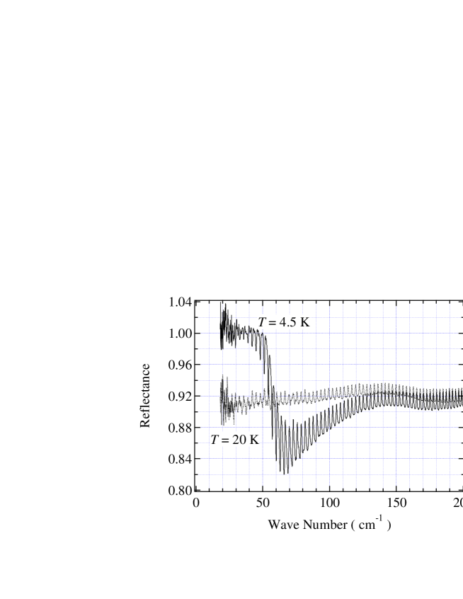
Figure 1: Reflectance spectra $R(\omega)$ of NbN_1-xC_x thin films deposited on MgO substrates at $T=4.3$ K (solid line) and $T=20$ K (dotted line).

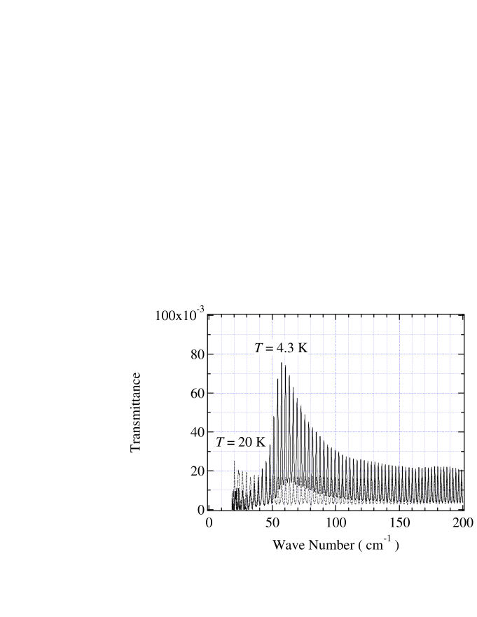
Figure 2: Transmittance spectra $T(\omega)$ of NbN_1-xC_x thin films deposited on MgO substrates at $T=4.3$ K (solid line) and 20 K (dotted line).

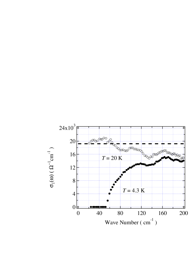
Figure 3: $\sigma_{1}(\omega)$ for NbN_1-xC_x calculated by the R-T method at $T=4.3$ K (solid circles) and $T=20$ K (open circles). The dashed line shows the results of calculations using the Drude formula at $T=20$ K.

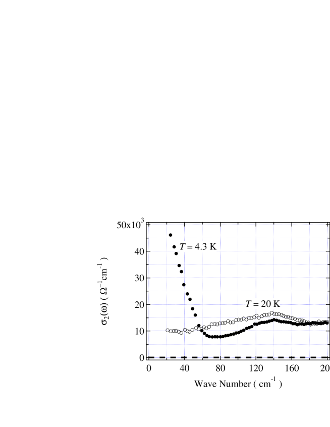
Figure 4: $\sigma_{2}(\omega)$ for NbN_1-xC_x calculated by the R-T method at $T=4.3$ K (solid circles) and $T=20$ K (open circles). The dashed line shows the results of calculations using the Drude formula at $T=20$ K.

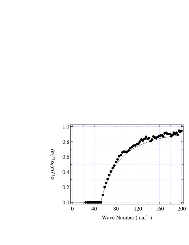
Figure 5: The relative conductivity ratio $\sigma_{1s}(\omega)/\sigma_{1n}(\omega)$ where $\sigma_{1}(\omega)$ at $T=4.3$ K is divided by $\sigma_{1}(\omega)$ at $T=20$ K. The solid line shows the results obtaned from the Mattis-Bardeen formula.

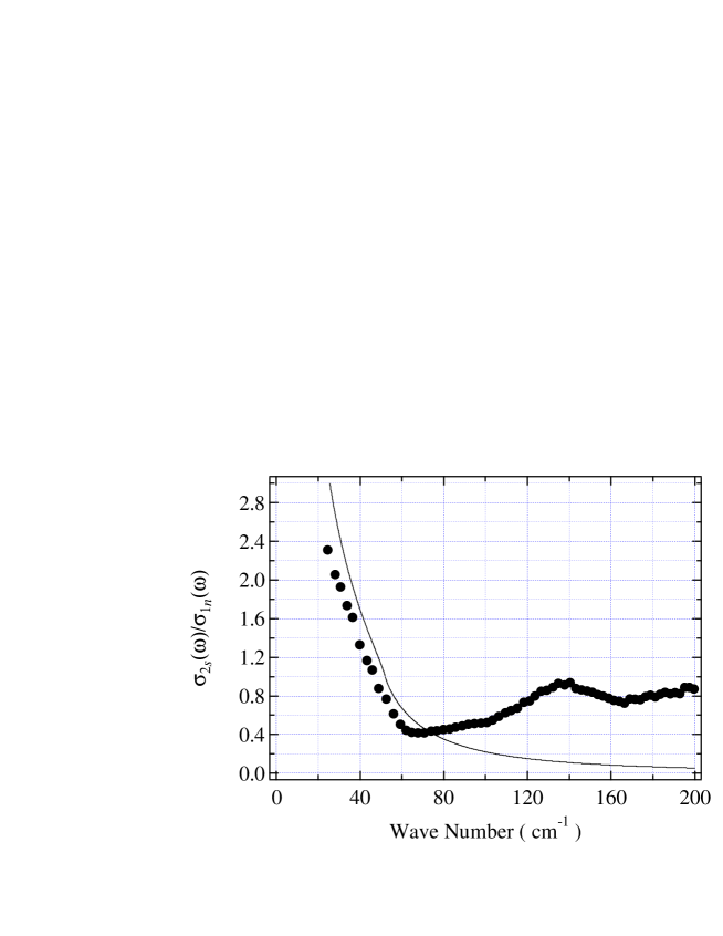
Figure 6: The relative conductivity ratio $\sigma_{2s}(\omega)/\sigma_{2n}(\omega)$ where $\sigma_{2}(\omega)$ at $T=4.3$ K is divided by $\sigma_{2}(\omega)$ at $T=20$ K. The solid line shows the results obtaned from the Mattis-Bardeen formula.

III.2 Experimental Results

In order to examine the feasibility of the R-T method, we report $R(\omega)$ and $T(\omega)$ of NbN_1-xC_x thin films deposited on MgO substrates in the far-infrared region. The substrates were 0.5 mm thick. The thickness of the NbN_1-xC_x layers was about 40 nm. The films were epitaxial and $T_{c}$ was estimated to be 17.5 K by electrical measurements. The value of $x$ was estimated to be less than 0.3.

The electrical resistivity measured by the four-probe method was $\rho=5.2\times 10^{-5}$ $\Omega$cm at $T=20$ K. The carrier density in the normal state $n$ was measured by the van der Pauw method: $n=1.29\times 10^{23}$ cm^-3 which is slightly lower than the value of $n=2.39\times 10^{23}$ cm^-3 reported previously for NbNmath72 . The carrier scattering rate $\Gamma$ at $T=20$ K was estimated as $\Gamma=\rho e^{2}n/m^{*}=1.9\times 10^{15}$ s^-1 = 6.3$\times 10^{4}$ cm^-1, where the effective mass $m^{*}$ is assumed to be equal to the electron rest mass. The superconducting gap has been estimated as $2\Delta\approx 50$ cm^-1. Thus NbN_1-xC_x is suggested to be a typical dirty-limit BCS superconductor.

$R(\omega)$ and $T(\omega)$ obtained at $T=4.3$ K and 20 K are shown in Figs. 1 and 2. The interference fringes due to multiple internal reflections within the MgO substrate are clearly visible in both figures because the MgO substrate is highly transparent in this $\omega$ region at $T=4.3$ K and 30 K, and because the NbN_1-xC_x film is thin enough to transmit far-infrared radiation. $R(\omega)$ at $T=4.3$ K exhibits an obvious reflectance edge at $\omega\sim 65$ cm^-1 and $R(\omega)\sim 1$ for $\omega$ less than the reflectance edge frequency, which is a special characteristic for superconductors. $T(\omega)$ at $T=4.3$ K exhibits a maximum at $\omega\sim 60$ cm^-1, which is related to the evolution of the reflectance edge in $R(\omega)$.

We show $\sigma_{1}(\omega)$ and $\sigma_{2}(\omega)$ spectra Figs. 3 and 4 for NbN_1-xC_x calculated by the R-T method using the experimental results shown in Figs. 1 and 2. The value of the dc conductivity $\sigma_{1}(0)$ at $T=20$ K is estimated to be $\sigma_{1}(0)\sim 2.0\times 10^{4}$ $\Omega^{-1}$cm^-1 from Fig. 3; this value agrees well with the value of $1/\rho=1.9\times 10^{4}$ $\Omega^{-1}$cm^-1 estimated from the electrical measurements.

We evaluated the relative conductivity ratio $\sigma_{1s}(\omega)/\sigma_{1n}(\omega)$ and $\sigma_{2s}(\omega)/\sigma_{1n}(\omega)$ from the results in Figs. 3 and 4, where $\sigma_{1n}$ is $\sigma_{1}$ at $T=20$ K and $\sigma_{1s}$ and $\sigma_{2s}$ are at $T=4.3$ K, respectively. The real and imaginary parts of the relative conductivity ratios are shown in Figs. 5 and 6, respectively. Here theoretical curves obtained using the Mattis-Bardeen theory are also shown by solid lines, where we set $2\Delta=52$ cm^-1 in accord with the value reported by the junction methodkoh99 . The ratio of $2\Delta$ to $T_{c}$ is given by $2\Delta/k_{B}T_{c}\sim 4.3$, suggesting the strong-coupling superconductivity in NbN_1-xC_x.

The experimental results for $\sigma_{1s}/\sigma_{1n}$ in Fig. 5 exhibit an excellent agreement with the Mattis-Bardeen theory, and $\sigma_{2s}/\sigma_{1n}$ also shows a good agreement for $\omega$ less than $\sim 60$ cm^-1 as shown in Fig. 6. The agreement is, however, poor for $\omega$ larger than $\sim 70$ cm^-1 in Fig. 6; this anomalous behavior may be due to impuritieszim91 .

Now we investigate the conductivity sum rule in eq.(91). From the integration of spectra $\sigma_{1n}$ and $\sigma_{1s}$, $\lambda_{L}$ was estimated to be $\sim 193$ nm, while the $\sigma_{2s}$ spectra in the superconducting state gives $\lambda_{L}\sim 200$ nm. These values show an excellent agreement, and also agrees well with the value reported previously.koh99 This indicates that the sum rule holds for NbN_1-xC_x.

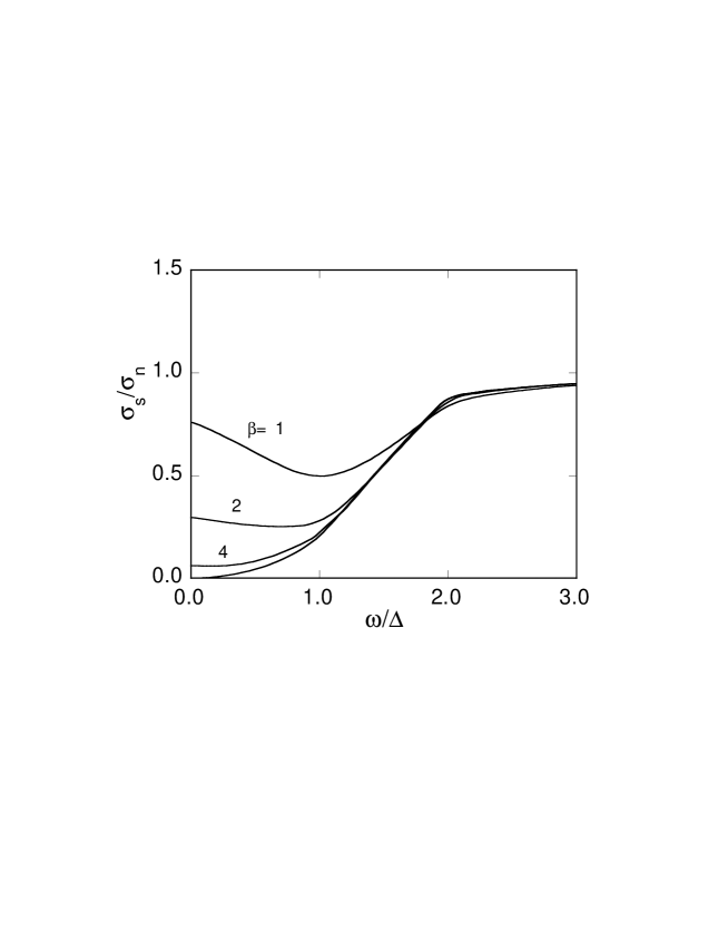
Figure 7: Real part of the optical conductivity as a function of $\omega$ for several values of temperature. From the top $T/\Delta=1/\beta=1,1/2,1/4$ and 0.

Figure 8: Optical conductivity calculated from the R-T method at $T=4.3$K (circles) and 30K (squares). The diamond indicates the DC value at $T=30$ K.

Figure 9: Optical conductivity (circles) by the R-T method and theoretical predictions at $T=0$ (solid curves). Form the left $2\Delta=50$cm^-1, 60$cm^{-1}$ and 70cm^-1

IV Electron-doped high-$T_{c}$ superconductor: London limit

Oxide high-$T_{c}$ superconductors have been investigated intensively over the last decade. The $d$-wave superconductivity is well established for hole-doped superconductors. However, there is a class of high-$T_{c}$ superconductors doped with electrons,tok89 ; tak89 for which both $s$-wavekas98 and $d$-wave pairingtsu00 ; kok00 ; pro00 have been reported. Nd_2-xCe_xCuO₄ is a typical example of electron-doped materials and the symmetry of Cooper pairs has been controversial. It is important to examine the symmetry of Cooper pairs in the study of high-$T_{c}$ superconductors.

Since the superconducting gap $\Delta$ in Nd_2-xCe_xCuO₄ is very small, there have been no reports on the study of the nature of the superconducting gap of Nd_2-xCe_xCuO₄ through such techniques, although there have been a number of reports on the FIR spectroscopy of Nd_2-xCe_xCuO₄.hom97 ; ono99

The purpose of this paper is to investigate FIR optical properties of Nd_2-xCe_xCuO₄ obtained by the R-T method from a viewpoint of unconventional superconductors. We will show that the available data for the optical conductivity and transmittance are well explained by $d$-wave pairing model in the clean limit. The value of superconducting gap is estimated as $2\Delta\sim 60-70$ cm^-1, which is consistent with the available value estimated by scanning tunneling spectroscopy.kas98

Figure 10: Observed Transmittance and the theoretical curves at $T=0$ (solid curve) for $2\Delta=60$cm^-1.

The frequency-dependent conductivity $\sigma(\omega)$ was calculated by Mattis and Bardeen,mat58 Abrikosov et al.abr59 and Skalski et al.ska64 for isotropic superconductors. The original Mattis-Bardeen theory was carried through for a conventional type-I $s$-wave superconductor, where the coherence length $\xi$ and magnetic penetration depth $\lambda$ satisfy $\xi\gg\lambda$. The opposite limit $\xi\ll\lambda$ (London limit) was also examined for $s$-wave pairing by field theoretical treatments.ska64 For the high-$T_{c}$ compounds of type-II superconductor with small coherence length, the formula in the London limit is appropriate for optical conductivity measurements. Recently the conductivity $\sigma(\omega)$ of an unconventional superconductor has been examined theoretically in the London limit.hir89 ; hir92 ; hir94 ; gra95 We use the current response function shown in Section II:

$$K_{\mu\nu}({\bf q},i\omega_{m})=\frac{e^{2}k_{F}^{2}}{m^{2}}\sum_{k}\hat{k}_{\mu}\hat{k}_{\nu}\frac{1}{\beta}\sum_{n}{\rm Tr}[G({\bf k}_{+},i\epsilon_{n}+i\omega_{m})G({\bf k}_{-},i\epsilon_{n})],$$ (114)

where ${\bf k}_{\pm}={\bf k}\pm{\bf q}/2$ and $\epsilon_{n}=(2n+1)\pi/\beta$. The single-particle matrix Green’s function is

$$G({\bf k},i\epsilon_{n})=\frac{i(\epsilon_{n}-\Sigma(\epsilon_{n}))\tau^{0}+\xi_{k}\tau^{3}+\Delta_{k}\tau^{1}}{(\epsilon_{n}-\Sigma(\epsilon_{n}))^{2}+\xi_{k}^{2}+\Delta_{k}^{2}},$$ (115)

where $\Delta_{k}$ is the anisotropic order parameter and $\Sigma(\epsilon_{n})$ is the self-energy due to impurity scattering. $\tau^{i}$ ($i=0,1,\cdots$) denote Pauli matrices. Since we consider the case where $\xi\ll\lambda$ holds, the real part of optical conductivity is well approximated by the formula in the London limit:

$$\sigma_{1s,\mu\nu}(\omega)=-\frac{1}{\omega}\lim_{q\rightarrow 0}{\rm Im}K_{\mu\nu}({\bf q},\omega).$$ (116)

Our focus is the collision less limit of the normalized conductivity to compare it with the data for Nd_2-xCe_xCuO₄ since $\xi\ll\ell$ holds for the mean-free path $\ell$. For anisotropic superconducting order parameter $\Delta_{k}$ such that the average over the Fermi surface vanishes $\langle\Delta_{k}\rangle=0$, the expression for $\sigma_{1s}\equiv\sigma_{1s,xx}(\omega)$ in the collision less limit on the plane is simply given byhir92

$$\frac{\sigma_{1s}(\omega)}{\sigma_{1n}(\omega)}=\frac{1}{2\omega}\int_{-\infty}^{\infty}dx\langle{\rm Re}\frac{|x|}{\sqrt{x^{2}-\Delta_{k}^{2}}}\rangle\langle{\rm Re}\frac{|x-\omega|}{\sqrt{(x-\omega)^{2}-\Delta_{k}^{2}}}\rangle[{\rm tanh}(\frac{\beta x}{2})-{\rm tanh}(\frac{\beta(x-\omega)}{2})],$$ (117)

which is an angle-dependent generalization of the Mattis-Bardeen formula. For the $d$-wave symmetry, the average over the Fermi surface denoted by the angular brackets is defined as

$$\langle{\rm Re}\frac{x}{\sqrt{x^{2}-\Delta_{k}^{2}}}\rangle={\rm Re}\int\frac{d\phi}{2\pi}\frac{x}{\sqrt{x^{2}-(\Delta{\rm cos}(2\phi))^{2}}},$$ (118)

where the order parameter is factorized as $\Delta_{k}=\Delta{\rm cos}(2\phi)$. In Fig.7 we show the behaviors of $\sigma_{1s}/\sigma_{1n}$ as a function of $\omega$ for several values of temperature $T$. The infrared behaviors reflect the lines of nodes on the Fermi surface.

FIR reflection $R(\omega)$ and transmission $T(\omega)$ measurements were performed for Nd_2-xCe_xCuO₄ ($x=0.15$) thin films deposited by laser ablation onto (001) MgO substrates. The thickness of Nd_2-xCe_xCuO₄ thin film was about 40 nm. $T_{c}$ was estimated to be $\sim$20K. The electric field of the FIR radiation was predominantly parallel to the $a$-$b$ plane. The conductivity spectra were evaluated by the R-T method from the data for $R(\omega)$ and $T(\omega)$ at $T=4.3$ and 30K.shi01

Figure 11: Transmission $T_{S}/T_{N}$ for anisotropic $s$-wave models. The solid curve without marks is the Mattis-Bardeen result. Squares, triangles and circles are for the prolate ($a=0.5$), ab-plane anisotropic ($c=0.5$), and oblate ($a=-0.5$) gaps, respectively. The oblate form shows a small increase compared to other types. For the oblate gap, $\Delta_{0}=\Delta_{max}$, and for other types, $\Delta_{0}=\Delta$.

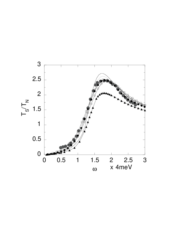
Figure 12: Transmission $T_{S}/T_{N}$ for the two-band model. The data points (large solid circles) are taken from ref.kai02 at $T=6$K. The solid line without marks shows the Mattis-Bardeen result with $2\Delta=5$meV. The dotted line is for the single gap of prolate type with $2\Delta_{max}=9$meV and $a=0.5$. Triangles are for the single-gap model of oblate form with $2\Delta_{max}=9$meV and $a=-0.33$. Others are for the two-band gap model where the ab-plane anisotropy for the $\sigma$-band and the prolate form for the $\pi$-band are assumed. The parameters are the following. Solid circles: $2\Delta_{max}=8.5$meV and $c=0.33$ ($\sigma$-band: weight 0.45); $2\Delta_{max}=6$meV and $a=0.33$ ($\pi$-band: weight 0.55). Open circles: $2\Delta_{max}=9$meV and $c=0.33$ ($\sigma$-band: weight 0.45); $2\Delta_{max}=6$meV and $a=0.33$ ($\pi$-band: weight 0.55). Squares: $2\Delta_{max}=10$meV and $c=0.5$ ($\sigma$-band: weight 0.4); $2\Delta_{max}=7.5$meV and $a=0.5$ ($\pi$-band: weight 0.6).

Figure 13: Specific-heat-jump ratio to the BCS value. From the top the ratios for the oblate, $ab$-anisotropy, and prolate gaps are shown, respectively.

Figure 14: Real part of the optical conductivity for the two-band anisotropic model. The data points (large solid circles) are taken from ref.kai02 The parameters for solid circles are $2\Delta_{max}=8.5$meV and $c=0.33$ ($\sigma$-band: weight 0.45); $2\Delta_{max}=6$meV and $a=0.33$ ($\pi$-band: weight 0.55). The parameters for open circles are $2\Delta_{max}=10$meV and $c=0.5$ ($\sigma$-band: weight 0.4); $2\Delta_{max}=7.5$meV and $a=0.5$ ($\pi$-band: weight 0.6). The dashed line indicates the results obtained using the Mattis-Bardeen formula with $2\Delta=5$meV. The dash-dotted line denotes the conductivity for the $d$-wave gap.yana01

Figure 15: Thermodynamic critical magnetic field $H_{c}(T)$ normalized by $H_{c}(T=0)_{BCS}$. The bold dashed curve indicates data from ref.bou01 and the bold solid curve indicates those obtained using the present two-band anisotropic model. The thin solid curve indicates the BCS results. The results for the $\sigma$-band (ab-plane anisotropic) and the $\pi$-band (prolate form) are also shown.

The R-T method provides us reliable data of spectroscopy in far-infrared region for which comparison between the experimental data and theoretical analysis is possible. In the R-T method both the reflectance spectra $R(\omega)$ and the transmittance spectra $T(\omega)$ are measured experimentally from which a set of coupled equations are followed describing the transmittance and reflectance of a thin film on a substrate. The coupled equations are solved numerically by the Newton method to determine the optical conductivity. This method is free from the difficulties in the infrared region which occur commonly in the conventional method employing a Kramers-Kronig transformation. In Fig.8, we show the real part of the optical conductivity obtained from the R-T method at $T=3.4$K and $T=30$K. In Fig.9 we show the observed data and theoretical curves at $T=0$ for $2\Delta=60$ and 70 cm^-1. The experimental data $\sigma(3.4K)/\sigma(30K)$ normalized by the normal state values at $T=30$K are shown in Fig.9. It is obvious from the experimental results that there is no evidence of a true gap, which is suggestive of anisotropic superconducting gap, since the spectral weight of conductivity should vanish for $\omega\leq 2\Delta$ at $T=0$ in conventional isotropic superconductors. It is also shown in Fig.9 that they are well fitted by the curve with $2\Delta=60$ cm^-1, which is consistent with the value estimated by scanning tunneling spectroscopy measurements.kas98

Transmission curve is also presented in Fig.10, where $T_{S}/T_{N}$, the ratio of the transmission in the superconducting to that in the normal state, is the experimentally measured quantity. The following expression for $T_{S}/T_{N}$ is employed to determine the transmission curve theoretically,glo57

$$\frac{T_{S}}{T_{N}}=\frac{1}{[T_{N}^{1/2}+(1-T_{N}^{1/2})(\sigma_{1}/\sigma_{n})]^{2}+[(1-T_{N}^{1/2})(\sigma_{2}/\sigma_{n})]^{2}},$$ (119)

where $\sigma_{1}$ and $\sigma_{2}$ are real and imaginary parts of the conductivity $-(c/\omega)K({\bf q},\omega)$ for ${\bf q}\rightarrow 0$, respectively. Here we use the formula obtained from the two-fluid model for $\sigma_{2}$. $T_{N}$ is determined as $T_{N}\simeq 0.05$ from the expression for the ratio of the power transmitted with a film to that with no film given as

$$T_{N}=1/[1+\sigma_{n}d\frac{Z_{0}}{n+1}]^{2}.$$ (120)

Here $d$ is the film thickness, $n$ is the index of refraction of the substrate, and $Z_{0}$ is the impedance of free space. We have assigned the following values; $d=4\times 10^{-6}$cm, $n=3.13$, $Z_{0}=377\Omega$ and $\sigma_{n}\approx 10^{4}\Omega^{-1}$cm^-1 and the Drude width is approximately equal to $\Delta$ $\sigma_{n}$ is approximately given by the value at $\omega=0$. Obviously the $\omega$-dependence of measured transmittance agrees with the theoretical curve for $2\Delta=60$cm^-1 as shown in Fig.10. An agreement between the observed quantities and theoretical curve is remarkable, which should be compared to the isotropic BCS prediction calculated from the Mattis-Bardeen equations.cho96

V Two-Band Anisotropic Superconductivity in Magnesium Diboride

After the discovery of 39 K superconductivity in MgB₂nag01 , much attention has been focused on the study of its nature. An $s$-wave superconductivity (SC) was established by experiments such as coherence peak in ¹¹B nuclear relaxation ratekot01 and its exponential dependence at low temperaturesyang01 ; man02 . An isotope effect has suggested phonon-mediated $s$-wave superconductivitybud01 .In contrast to its standard properties, there have been several reports indicating unusual properties of the superconductivity of MgB₂. Two different superconducting gaps have been reported: a gap much smaller than the expected BCS value and that comparable to the BCS value given by $2\Delta=3.53k_{B}T_{c}$. Their ratio is estimated to be $\Delta_{min}/\Delta_{max}\sim 0.3-0.4$ using several experimentsyang01 ; tsu01 ; sza01 ; che01 ; giu01 ; bou01 . It is also reported that the specific-heat jump and the critical magnetic field are reduced compared to the $s$-wave BCS theoryyang01 ; bou01 . A strongly anisotropic upper critical field in $c$-axis-oriented MgB₂ films and single crystals of MgB₂ is also observedlim01 ; xu01 ; ang02 .

Table 1: Anisotropic parameters in the SC gap function used to fit several physical quantities. The upper four rows are for the single-SC gap model and the last row is for the two-band anisotropic model for comparison. The cross indicates that we cannot fit experimental data by the corresponding $z$ factor. $\Delta$ in the column $H_{c2}$ indicates that experiments are explained qualitatively but not quantitatively.haa01 The big circle show that we can fit the data using the same parameters in the column $\sigma_{1}$. The effect of $\sigma$-band anisotropy is small.

	$z$	$\sigma_{1}$	$T_{S}/T_{N}$	$\Delta C$	$H_{c}(0)$	$H_{c2}$
Cigar-type	$1+a{\rm cos}(2\theta)$	$a\sim 0.5$	$\sim 0.3$	$\sim 0.3$	$\sim 0.07$	$\times$
Pancake	$1-a^{\prime}{\rm cos}(2\theta)$	$a^{\prime}\sim 0.6$	$\times$	$\sim 0.5$	$\times$	$\Delta$
Pancake	$1-b{\rm cos}^{2}(\theta)$	$b\sim 0.75$	$\times$	$\sim 0.66$	$\sim 0.08$	$\Delta$
In-plane	$1+c{\rm cos}(6\phi)$	$c\sim 0.5$	$\sim 0.3$	$\sim 0.3$	$\times$
Two-band	($\sigma$ band)	$c<0.3$	$\bigcirc$	$\bigcirc$	$\bigcirc$
	($\pi$ band)	$a\sim 0.3$

The unusual properties of MgB₂ suggest an anisotropic $s$-wave superconductivity or a two-band superconductivity. The band structure calculations predicted multibands originating from $\sigma(2p_{x,y})$ and $\pi(2p_{z})$ bands.kor01 In the ARPES measurements performed in single crystals of MgB₂ three distinct dispersions approaching the Fermi energy were reported.uch02

There have been several studies on the anisotropy of a superconducting gaphaa01 ; mir02 ; nak02 ; tew02 ; bou02 . The two-gap model is shown to consistently describe the specific heatnak02 ; bou02 and the upper critical field $H_{c2}$mir02 with the adoption of the effective mass approach.

Here we show that this material is described by two order parameters attached to $\sigma$- and $\pi$-bands. Two order parameters further must have different anisotropy to explain the experimental results consistently. In this paper, we examine optical properties and thermodynamics to determine the k-dependence of the gaps. We show that the optical transmittance, conductivity, specific-heat jump, and thermodynamic critical field $H_{c}$ are well described by a two-band superconductor model with different anisotropies in ${\bf k}$-space. The symmetry in ${\bf k}$-space is determined in order to explain these experiments consistently.

The optical conductivity for anisotropic s-wave SC is investigated and compared with available data for MgB₂. A simple angle-dependent generalization of the Mattis-Bardeen formulamat58 is used to calculate the optical conductivity. The density of states $N(\epsilon)=\epsilon/\sqrt{\epsilon^{2}-\Delta^{2}}$ is generalized to $N(\epsilon)=\langle{\rm Re}\epsilon/\sqrt{\epsilon^{2}-\Delta_{{\bf k}}^{2}}\rangle_{k}$, where the bracket indicates the average over the Fermi surface. We employed the following formula at T=0:

$$\frac{\sigma_{1s}}{\sigma_{1n}}(\omega)=\frac{1}{\omega}\int_{0}^{\omega}dE[N(E)N(\omega-E)-\langle{\rm Re}\frac{\Delta_{\bf k}}{\sqrt{E^{2}-\Delta_{\bf k}^{2}}}\rangle_{k}\langle{\rm Re}\frac{\Delta_{\bf k^{\prime}}}{\sqrt{(\omega-E)^{2}-\Delta_{{\bf k^{\prime}}}^{2}}}\rangle_{k^{\prime}}],$$ (121)

$$\frac{\sigma_{2s}}{\sigma_{1n}}(\omega) = -\frac{1}{\omega}\int^{\omega+\Delta_{max}}_{\Delta_{min}}dE[\langle{\rm Re}\frac{E}{\sqrt{E^{2}-\Delta_{k}^{2}}}\rangle_{k}\langle{\rm Re}\frac{\omega-E}{\sqrt{\Delta_{k^{\prime}}^{2}-(\omega-E)^{2}}}\rangle_{k^{\prime}}$$ (122)

$$- \langle{\rm Re}\frac{\Delta_{k}}{\sqrt{E^{2}-\Delta_{k}^{2}}}\rangle_{k}\langle{\rm Re}\frac{\Delta_{k^{\prime}}}{\sqrt{\Delta_{k^{\prime}}^{2}-(\omega-E)^{2}}}\rangle_{k^{\prime}}].$$

We here mention that if the samples are clean and belong to the category of London superconductors, we must use the formulas in the London limit. For a clean superconductor, it seems better to use $\sigma_{2s}$ for the two-fluid modelshi03 . The optical data that we will consider here exhibit behaviors explained by the conventional formulas of Mattis and Bardeen. The anisotropic order parameters considered in this paper are:

$$\Delta_{c1}({\bf k}) = \Delta(1+a{\rm cos}(2\theta)),$$

$$\Delta_{c2}({\bf k}) = \Delta(1-b{\rm cos}^{2}(\theta)),$$

$$\Delta_{ab}({\bf k}) = \Delta(1+c{\rm cos}(6\phi)).$$ (123)

Here, $\theta$ and $\phi$ are the angles in the polar coordinate where $\theta$ is the polar angle with respect to the c-axis. The parameters $a$, $b$ and $c$ determine the anisotropy. $\Delta_{c1}$ is a prolate form gap for $a>0$ and is oblate for $a<0$. $\Delta_{c2}$ ($b>0$) shows the same anisotropy as $\Delta_{c1}$ for $a<0$. $\Delta_{ab}({\bf k})$ indicates an anisotropy in the $ab$-plane; the SC gap may possibly be anisotropic in the plane since the 2D-like Fermi surface has a hexagonal symmetry.kor01 The integral in eq.(121) is evaluated numerically by writing the average over the Fermi surface with elliptic functions. For example, for $\Delta_{c1}({\bf k})=\Delta(1+a{\rm cos}(2\theta))$, the average over the Fermi surface for $0<a<1$ is given by

$$\langle{\rm Re}\frac{\omega}{\sqrt{\omega^{2}-\Delta_{c1}({\bf k})^{2}}}\rangle = \frac{1}{2}\sqrt{\frac{\omega}{a\Delta}}F\left(\frac{\pi}{2},k\right),~{}~{}(1-a)\Delta\leq\omega\leq(1+a)\Delta,$$ (124)

$$= \frac{1}{2}\sqrt{\frac{\omega}{a\Delta}}F\left(\gamma,k\right),~{}~{}(1+a)\Delta<\omega,$$

where $k^{2}=(\omega-(1-a)\Delta)/(2\omega)$, $\gamma={\rm sin}^{-1}\sqrt{4a\Delta\omega/[(\omega-(1-a)\Delta)(\omega+(1+a)\Delta)]}$ and $F(\gamma,k)$ is the elliptic integral of the first kind.

Table 2: Several physical quantities obtained by the two-band model with $c\sim 0.33$ ($\sigma$ band) and $a\sim 0.33$ ($\pi$ band).

	$w_{\sigma}/w_{\pi}$	$\Delta_{min}/\Delta_{max}$	$\frac{\Delta C(T_{c})}{\Delta C(T_{c})_{BCS}}$	$\frac{H_{c}(0)}{H_{c}(0)_{BCS}}$
Two-band	0.45/0.55	$\sim 0.35$	$\sim 0.82$	$\sim 0.95$
Exp.	0.45/0.55	$0.3-0.4$	$0.76-0.92$	0.96

First, we examine a one-band anisotropic model and show that the one-band model is insufficient to understand consistently optical and thermodynamic behaviors. In Fig. 11 the transmission $T_{S}$ at $T=0$ is shown as a function of the frequency $\omega$.yan03b We again employ the following phenomenological expression for $T_{S}/T_{N}$yana01 ; glo57 ,

$$\frac{T_{S}}{T_{N}}=\frac{1}{[T_{N}^{1/2}+(1-T_{N}^{1/2})(\sigma_{1}/\sigma_{n})]^{2}+[(1-T_{N}^{1/2})(\sigma_{2}/\sigma_{n})]^{2}},$$ (125)

where $\sigma_{1}$ and $\sigma_{2}$ are real and imaginary parts of the optical conductivity, respectively. $T_{N}$ is determined from the expression for the ratio of the power transmitted with a film to that transmitted without a film given as $T_{N}=1/[1+\sigma_{n}dZ_{0}/(n+1)]^{2}$. Here, $d$ is the film thickness, $n$ is the index of refraction of the substrate, and $Z_{0}$ is the impedance of free space. We have assigned the following values: $d=10^{-6}$ cm, $n\approx 3$, $Z_{0}=377\Omega$, and $\sigma_{n}\approx 8\times 10^{3}\Omega^{-1}$cm^-1. Then we obtain $T_{N}\simeq 0.014$. The theoretical curves for $T_{S}/T_{N}$ are shown in Fig. 11; they have peaks near $\omega\sim 2\Delta_{0}$. For the oblate, its peak shows an increase only twice the normal state value, while the prolate and ab-plane anisotropies show more than twofold increases. The experiments show an approximately 2.5-fold increasekai02 which supports the prolate or ab-plane anisotropic symmetry. However, the temperature dependence of the ratio $H_{c2}^{ab}/H_{c2}^{c}$, which increases as the temperature decreasesang02 , indicates that $\Delta({\bf k})$ has an oblate form instead of a prolate formhaa01 in contrast to $T_{S}/T_{N}$. It is also difficult to describe the thermodynamic quantities such as the specific-heat jump at $T=T_{c}$ and the thermodynamic critical magnetic field $H_{c}$ within the single-gap model consistently. The specific-heat jump at $T_{c}$ is given by

$$\frac{\Delta C(T_{c})}{\gamma_{C}T_{c}}=\frac{12}{7\zeta(3)}\frac{\langle z^{2}\rangle^{2}}{\langle z^{4}\rangle},$$ (126)

where $\gamma_{C}$ is the specific-heat coefficient and $z$ is an anisotropic factor of the gap function. $\langle z^{n}\rangle$ is the average of $z^{n}$ over the Fermi surface. In Fig. 13 the specific-heat-jump ratio vs anisotropy ($a$ or $c$) is shown. The experiments indicate that this value is in the range of 0.76$\sim$ 0.92yan01 ; bou01 ; the fitting parameters must be $a\sim 0.3$, $-a\sim 0.5$ and $c\sim 0.3$ for the prolate, oblate and ab-anisotropic types, respectively. We must assign different values to parameters $a$ and $c$ in order to explain the thermodynamic critical magnetic field $H_{c}$. The ratio of $H_{c}(T=0)$ to the BCS value is given as

$$\frac{H_{c}(T=0)^{2}}{\gamma_{C}T_{c}^{2}}=\frac{6\pi}{{\rm e}^{2\gamma}}\langle z^{2}\rangle=5.94\langle z^{2}\rangle.$$ (127)

Thus to be consistent with the experimental resultsbou01 , $\langle z^{2}\rangle$ should be less than 1; $a$ should be small, $a\sim 0.07$, for the prolate form, and the ab-plane anisotropic and oblate forms $(a<0$) are ruled out since $\langle z^{2}\rangle>1$. In Table I, we summarize the status for the single-gap anisotropic $s$-wave model applied to MgB₂. As shown here, it is difficult to understand the physical behaviors measured using several experimental methods consistently within the single-gap model.

Here, a two-band model with two different anisotropies is investigated. We assume that the hybridization between $\sigma$ and $\pi$ bands is negligible, and that the optical conductivity is given by

$$\sigma=w_{\sigma}\sigma_{\sigma}+w_{\pi}\sigma_{\pi},$$ (128)

where $\sigma_{\sigma}$ and $\sigma_{\pi}$ denote the contributions from $\sigma$- and $\pi$-bands, respectively. For the case of isotropic two gaps, $\sigma_{1}$ must have a shoulder-like structure which appear as an addition of two contributions from the two bands, if the magnitudes of two SC gaps are different. The experimental data of $\sigma_{1}$, however, does not have such a sharp structure (see Fig. 14).kai02 ; lee02 Therefore we must take account of anisotropies for the two-band model. We assume the in-plane anisotropy for the two-dimensional-like $\sigma$-band, while we assign the three-dimensional anisotropy to $\pi$-band where the prolate and oblate forms are examined.

The transmission $T_{S}/T_{N}$ in Fig. 12 shows that the theoretical curve is in good agreement with the experimental curve. The optical conductivity is also described well by the two-band model as shown in Fig. 14. We assign the following parameters to the best fit model in Figs. 12 and 14; the $\sigma$-band has ab-plane anisotropy with $c\approx$ or less than 0.33 and the $\pi$-band has the prolate form gap (cigar type) with $a\approx 0.33$. The ratio of the weight of the $\sigma$-band to that of the $\pi$-band is 0.45/0.55, which agrees with penetration depthman02 and band structure calculationsbel01 . The ratio of the minimum gap to the maximum gap is 0.35, which is in the range of previously reported experimental values.tsu01 ; giu01 Let us mention that the effect of $\sigma$-band anisotropy is small for the transmission $T_{S}/T_{N}$.

In Fig. 15 the thermodynamic critical magnetic field $H_{c}(T)$ is shown for the single-band and two-band models with available data.bou01 We have simply assumed that the total free energy is given by the sum of two contributions from $\sigma$- and $\pi$-bands: $\Omega=w_{\sigma}\Omega_{\sigma}+w_{\pi}\Omega_{\pi}$. The experimental behavior is well explained by the two-band anisotropic model using the same parameters as those for $T_{S}/T_{N}$ and $\sigma_{1s}/\sigma_{1n}$. We show several characteristic values obtained from the two-band model in Table II.

Let us mention here that the two-gap model shows consistency concerning other physical quantities. Results of analyses of $H_{c2}$ and specific heat using the effective mass approach are consistent with those obtained using the two-band model.mir02 ; nak02 ; bou02 It has been reported that the increasing nature of $H_{c2,ab}/H_{c2,c}$ with decreasing temperature is explained by the two-Fermi surface model.mir02 The specific-heat coefficient $\gamma$ in magnetic fields seems consistent with that of the multiband superconductor.nak02 ; bou02

VI Summary

We have discussed the optical properties in unconventional superconductors. Theoretical aspects of the conductivity were discussed in detail from the linear response theory to the formula in the London limit. We have presented a new method (R-T method) to measure $\sigma(\omega)$ in the far-infrared region from reflectance and transmittance data without the use of the Kramers-Kronig transformations. This method provides a method to obtain the far-infrared properties more precisely compared to the conventional method. The conductivity sum rule is discussed briefly. It has been reported that the sum rule is satisfied for the optical conductivity spectra of NbN_1-xC_x that is a typical conventional superconductor.

We have successfully made a comparison between experiments and theory for the optical conductivity of Nd_2-xCe_xCuO₄ in the far-infrared region. We have shown that there is a reasonable agreement between the optical conductivity $\sigma_{1}(\omega)$ observed by the R-T method and theoretical analysis without adjustable parameters except the superconducting gap. An estimate of 60$\sim$70 cm^-1 for the superconducting gap is consistent from both the experimental and theoretical aspects. The far-infrared optical conductivity suggests that the superconducting gap of electron-doped Nd_2-xCe_xCuO₄ is unconventional one with nodes on the Fermi surface. The anisotropic nature of electron-doped superconductors is consistent with the recent research performed for the one-band and three-band Hubbard models.yam98 ; kur99 ; yan01 ; yan02 ; yan03 If the superconducting gap is anisotropic for the electron-doped superconductors, there is a possibility that both the hole-doped and electron-doped cuprates superconductors are governed by a same superconductivity mechanism.

We have also examined the transmittance, optical conductivity, specific-heat jump and thermodynamic critical magnetic field $H_{c}$ of MgB₂ based on the two-band anisotropic $s$-wave model. This material is described by two order parameters attached to $\sigma$- and $\pi$-bands, respectively, which, moreover, have further anisotropy. We have shown that the two-gap model with different anisotropy in ${\bf k}$-space can explain the experimental results consistently.

VII acknowledgment

We express our sincere thanks to our coworkers: E. Kawate, S. Kimura, S. Kashiwaya, A. Sawa and S. Kohjiro. We thank Professor K. Maki for comments on the London superconductor.

References

- (1) A. A. Abrikosov, Fundamentals of the Theory of Metals (North-Holland, Amsterdam, 1988).
- (2) A. A. Abrikosov, L.P. Gorkov, and I.M. Khalatnikov, JETP 8, 1090 (1959) .
- (3) M. Angst, R. Puzniak, A. Wisniewski, J. Jun, S. M. Kazakov, J. Karpinski, J. Roos and H. Keller, Phys. Rev. Lett. 88, 167004 (2002).
- (4) D. N. Basov et al., Science 283, 49 (1999).
- (5) K. D. Belashchenko, M. van Schilfgaarde and V. P. Antropov, Phys. Rev. B64, 092503 (2001).
- (6) F. Bouquet, R. A. Fisher, N. E. Philips, D. G. Hinks and J. D. Jorgensen, Phys. Rev. Lett. 87, 047001 (2001).
- (7) F. Bouquet, Y. Wang, I. Sheikin, T. Plackowski, A. Junod, S. Lee and S. Tajima, Phys. Rev. Lett. 89, 257001 (2002).
- (8) S. L. Bud’ko, G. Lapertot, C. Petrovic, C. E. Cunningham, N. Anderson and P. C. Canfield, Phys. Rev. Lett. 86, 1877 (2001).
- (9) X. K. Chen, M. J. Konstantinovic, J. C. Irwin, D. D. Lawrie and J. P. Frank, Phys. Rev. Lett. 87, 157002 (2001).
- (10) E-J. Choi, K.P. Stewart, S.K. Kaplan, H.D. Drew, S.N. Mao, and T. Venkatessan, Phys. Rev. B53, 8859 (1996).
- (11) B. Dora, K. Maki and A. Virosztek, cond-mat/0012198.
- (12) B. Dora, K. Maki and A. Virosztek, Euro. Phys. Lett. 62, 426 (2003).
- (13) F. Gao, D.B. Romero, D.B. Tanner, J. Talvacchio, M.G. Forrester, Phys. Rev. B47, 1036 (1993).
- (14) F. Giubileo, D. Roditchev, W. Sacks, R. Lamy, D.X. Thanh, J. Klein, S. Miraglia, D. Fruchart, J. Marcus and Ph. Monod, Phys. Rev. Lett. 87, 177008 (2001).
- (15) R.E. Glover and M. Tinkham, Phys. Rev. 108, 243 (1957).
- (16) M.J. Graf, M. Mario, D. Rainer, and J.A. Sauls, Phys. Rev. B52, 10588 (1995).
- (17) S. Haas and K. Maki, Phys. Rev. B65, 020502 (2001).
- (18) P.J. Hirschfeld, P. Wölfle, J.A. Sauls, D. Einzel, and W.O. Putikka, Phys. Rev. B40, 6695 (1989).
- (19) P.J. Hirschfeld, W.O. Putikka, P. Wölfle, and Y. Campbell, J. Low Temp. Phys. 88, 395 (1992).
- (20) P.J. Hirschfeld, W.O. Putikka, and D.J. Scalapino, Phys. Rev. B50, 10250 (1994).
- (21) C.C. Homes, B.P. Clayman, J.L. Peng, and R.L. Greene, Phys. Rev. B56, 5525 (1997).
- (22) J. R. Jasperse, A. Kahan, J. N. Plendl and S. S. Mitra, Phys. Rev. 146, 146 (1966).
- (23) T. R. Yang, S. Perkowitz, G. L. Carr, R. C. Budhani, G. P. Williams and C. J. Hirschmugl, Appl. Opt. 29, 332 (1990).
- (24) R. A. Kaindl, M. A. Carnahan, J. Orenstein and D. S. Chemla, Phys. Rev. Lett. 88, 027003 (2002).
- (25) S. Kashiwaya, T. Ito, K. Oka, S. Ueno, H. Takashima, M. Koyanagi, Y. Tanaka, and K. Kajimura, Phys. Rev. B57, 8680 (1998).
- (26) E. Kawate, Physica B329-333, 1431 (2003).
- (27) M. Koguchi et al., Meeting Abstracts of the 53rd Annual Meeting of the Physical Society of Japan 53, 614 (1998).
- (28) S. Kohjiro and A. Shoji, Inst. Phys. Conf. Ser. No. 167, 655 (1999).
- (29) J.D. Kokales, P. Fournier, L.V. Mercaldo, V.V. Talanov, R.L. Greene, and S.M. Anlage, Phys. Rev. Lett. 85, 3696 (2000).
- (30) J. Kortus, I. I. Mazin, K. D. Belashchenko, V. P. Antropov and L. L. Boyer, Phys. Rev. Lett. 86, 4656 (2001).
- (31) H. Kotegawa, K. Ishida, Y. Kitaoka, T. Muranaka and J. Akimitsu, Phys. Rev. Lett. 87, 127001 (2001).
- (32) K. Kuroki, R. Arita, and H. Aoki, J. Low Temp. Phys. 117, 247 (1999).
- (33) H.J. Lee, J.H. Jung, K.W. Kim, M.W. Kim, T.W. Noh, Y.J. Wang, W.N. Kang, E.-M. Choi, H.-J. Kim, and S.-I. Lee, Phys. Rev. B65, 224519 (2002).
- (34) O. F. de Lima, C. A. Cardoso, R. A. Ribeiro, M. A. Avilla and A. A. Coelho, Phys. Rev. B64, 144517 (2001).
- (35) F. Manzano, A. Carrington, N. E. Hussey, S. Lee, A. Yamamoto and S. Tajima, Phys. Rev. Lett. 88, 047002 (2002).
- (36) D.C. Mattis and J. Bardeen, Phys. Rev. 111, 412 (1958).
- (37) M. P. Mathur, D. W. Deis and J. R. Gavaler, J. Appl. Phys. 43, 3138 (1972).
- (38) P. Miranovic, K. Machida and V.G. Kogan, J. Phys. Soc. Jpn. 72, 221 (2003).
- (39) J. Nagamatsu, N. Nakagawa, T. Muranaka, Y. Zenitani and J. Akimitsu, Nature 410, 63 (2001).
- (40) N. Nakai, M. Ichioka and K. Machida, J. Phys. Soc. Jpn. 71, 23 (2002).
- (41) M. R. Norman and C. Pepin, Phys. Rev. B66, 100506 (2002).
- (42) P. Nozieres and D. Pines, Theory of Quantum Liquids ( Advanced Book Classics, Harpercollins, 1999).
- (43) Y. Onose, Y. Taguchi, T. Ishikawa, S. Shinomori, K. Ishizuka, and Y. Tokura, Phys. Rev. Lett. 82, 5120 (1999).
- (44) R. Prozorov, R.W. Gianetta, P. Fournier, and R.L. Greene, Phys. Rev. Lett. 85, 3700 (2000).
- (45) S. Skalski, O. Betbeder-Matibet, and P.R. Weiss, Phys. Rev. 136, A1500 (1964).
- (46) H. Shibata, K. Shinji, S. Kashiwaya, S. Ueno, M. Koyanagi, N. Terada, E. Kawate and Y. Tanaka, Jpn. J. Appl. Phys. 40, 3163 (2001).
- (47) H. Shibata, S. Kimura, S. Kashiwaya, S. Kohjiro, A. Sawa, K. Mitsugi and Y. Tanaka, Physica C367, 337 (2002).
- (48) H. Shibata et al., in Proceedings of The 23rd International Conference on Low Temperature Physics (Hiroshima, 2002).
- (49) P. Szabo, P. Samuely, J. Kacmarcik, T. Klein, J. Marcus, D. Fruchart, S. Miraglia, C. Marcenat and A. G. M. Jansen, Phys. Rev. Lett. 87, 137005 (2001) .
- (50) H. Takagi, S. Uchida, and Y. Tokura, Phys. Rev. Lett. 62, 1197 (1989).
- (51) L. Tewordt and D. Fay, Phys. Rev. Lett. 89, 137003 (2002).
- (52) T. Timusk and D.B. Tanner, in Physical Properties of High-Temperature Superconductivity I, edited by D.M. Ginsberg (World Scientific, Singapore, 1989).
- (53) M. Tinkham and R. A. Ferrell, Phys. Rev. Lett. 2, 331 (1959).
- (54) Y. Tokura, H. Takagi, and S. Uchida, Nature 337, 345 (1989).
- (55) S. Tsuda, T. Yokoya, T. Kiss, Y. Takano, K. Togano, H. Kito, H. Ihara and S. Shin, Phys. Rev. Lett. 87, 177006 (2001).
- (56) C.C. Tsuei and J.R. Kirtley, Phys. Rev. Lett. 85, 182 (2000).
- (57) M. Xu, H. Kitazawa, Y. Takano, J. Ye, K. Nishida, H. Abe, A. Matsushita, N. Tsuji and G. Kido, Appl. Phys. Lett. 79, 2779 (2001).
- (58) H. Uchiyama, K. M. Shen, S. Lee, A. Damascelli, D. H. Lu, D. L. Feng, Z. X. Shen, and S. Tajima, Phys. Rev. Lett. 88, 157002 (2002).
- (59) K. Yamaji, T. Yanagisawa, T. Nakanishi and S. Koike, Physica C 304, 225 (1998).
- (60) T. Yanagisawa, S. Koike, and K. Yamaji, Phys. Rev. B64, 184509 (2001).
- (61) T. Yanagisawa, S. Koikegami, H. Shibata, S. Kimura, S. Kashiwaya, A. Sawa, N. Matsubara and K. Takita, J. Phys. Soc. Jpn. 70, 2833 (2001).
- (62) T. Yanagisawa, S. Koike, M. Miyazaki, and K. Yamaji, J. Phys. Condens. Matter 14, 21 (2002).
- (63) T. Yanagisawa, M. Miyazaki, S. Koikegami, S. Koike, and K. Yamaji, Phys. Rev. B67, 132408 (2003).
- (64) T. Yanagisawa and H. Shibata, J. Phys. Soc. Jpn. 72, 1619 (2003).
- (65) H.D. Yang, J.Y. Lin, H.H. Li, F.H. Hsu, C.J. Liu, S.C. Li, R.C. Yu, and C.Q. Jin, Phys. Rev. Lett. 87, 167003 (2001).
- (66) W. Zimmermann, E. H. Brandt, M. Bauer, E. Seider and L. Genzel, Physica C183, 99 (1991).