Quantifying signals with power-law correlations: A comparative study of
detrended fluctuation analysis and detrended moving average techniques

Abstract

Detrended fluctuation analysis (DFA) and detrended moving average (DMA) are two scaling analysis methods designed to quantify correlations in noisy non-stationary signals. We systematically study the performance of different variants of the DMA method when applied to artificially generated long-range power-law correlated signals with an a-priori known scaling exponent $\alpha_{0}$ and compare them with the DFA method. We find that the scaling results obtained from different variants of the DMA method strongly depend on the type of the moving average filter. Further, we investigate the optimal scaling regime where the DFA and DMA methods accurately quantify the scaling exponent $\alpha_{0}$, and how this regime depends on the correlations in the signal. Finally, we develop a three-dimensional representation to determine how the stability of the scaling curves obtained from the DFA and DMA methods depends on the scale of analysis, the order of detrending, and the order of the moving average we use, as well as on the type of correlations in the signal.

I introduction

There is growing evidence that output signals of many physical Robinson03 ; Ivanova03 ; Siwy02 ; Varotsos1 ; Varotsos2 ; Bundeatm ; talknertem2000 ; Eichner03 ; Fraedrich ; Pattantyus04 ; Montanari2000 ; Matsoukas2000 ; Moret ; Kavasseri ; Zebende , biological CKDFA1 ; SVDFA1 ; mantegnaprl1996 ; CarpenaNature02 , physiological  iyengaramjphsiolreg ; suki2002 ; plamenuropl1999 ; Pikkujamsaheartcir1999 ; crossoverCK ; toweillheartmed2000 ; bundesleep2000 ; Yosef2001 ; plamenchaos2001 ; janpresleep02 ; Karasik ; Echeverria ; KantelhardtEurophy03 ; huphysica04 ; suki2004 ; Hwa and economic systems vandewallepre1998 ; Liu99 ; janosiecopha1999 ; ausloosphsa1999_12 ; robertoecopha1999 ; grau-carles2000 ; ausloospre2001 ; Ivanovpre2004 , where multiple component feedback interactions play a central role, exhibit complex self-similar fluctuations over a broad range of space and/or time scales. These fluctuating signals can be characterized by long-range power-law correlations. Due to nonlinear mechanisms controlling the underlying interactions, the output signals of complex systems are also typically non-stationary, characterized by embedded trends and heterogeneous segments (patches with different local statistical properties) kunpre2001 ; zhipre2002 ; zhipre2004 . Traditional methods such as power-spectrum and auto-correlation analysis non ; hurst1 ; mandelbrot1 are not suitable for non-stationary signals.

Recently, new methods have been developed to address the problem of accurately quantifying long-range correlations in non-stationary fluctuating signals: (a) the detrended fluctuation analysis (DFA) CKDFA1 ; crossoverCK ; taqqu95 , and (b) the detrended moving average method (DMA) ANNApre2004 ; ANNADMA2 ; Spie2 ; BBak ; Annaphysica2004 . An advantage of the DFA method  kunpre2001 ; zhipre2002 ; zhipre2004 ; Wilson is that it can reliably quantify scaling features in the fluctuations by filtering out polynomial trends. However, trends may not necessarily be polynomial, and the DMA method was introduced to estimate correlation properties of non-stationary signals without any assumptions on the type of trends, the probability distribution, or other characteristics of the underlying stochastic process.

Here, we systematically compare the performance of the DFA and different variants of the DMA method. To this end we generate long-range power-law correlated signals with an a-priori known correlation exponent $\alpha_{0}$ using the Fourier filtering method MFFM . Tuning the value of the correlation exponent $\alpha_{0}$, we compare the scaling behavior obtained from the DFA and different variants of the DMA methods to determine: (1) how accurately these methods reproduce $\alpha_{0}$; (2) what are the limitations of the methods when applied to signals with small or large values of $\alpha_{0}$. Based on single realization as well as on ensemble averages of a large number of artificially generated signals, we also compare the best fitting range (i.e. the minimum and the maximum scales) over which the correlation exponent $\alpha_{0}$ can be reliably estimated by the DFA and DMA methods.

The outline of this paper is as follows. In Sec. II, we review the DFA method and we introduce variants of the DMA method based on different types of moving average filters. In Sec. III we compare the performance of DFA and DMA on correlated and anti-correlated signals. We also test and compare the stability of the scaling curves obtained by these methods by estimating the local scaling behavior within a given window of scales and for different scaling regions. In Sec. IV we summarize our results and discuss the advantages and disadvantages of the two methods. In Appendix I we consider higher order weighted detrended moving average methods, and in Appendix II we discuss moving average techniques in the frequency domain.

II Methods

II.1 Detrended Fluctuation Analysis

The DFA method is a modified root-mean-square (rms) analysis of a random walk. Starting with a signal $u(i)$, where $i=1,...,N$, and $N$ is the length of the signal, the first step of the DFA method is to integrate $u(i)$ and obtain

$$y(i)=\sum_{j=1}^{i}(u(j)-\bar{u}),$$ (1)

where

$$\bar{u}\equiv\frac{1}{N}\sum_{j=1}^{N}u(j)$$ (2)

is the mean.

The integrated profile $y(i)$ is then divided into boxes of equal length $n$. In each box $n$, we fit $y(i)$ using a polynomial function $y_{n}(i)$, which represents the local trend in that box. When a different order of a polynomial fit is used, we have a different order DFA-$\ell$ (e.g., DFA-1 if $\ell=1$, DFA-2 if $\ell=2$, etc).

Next, the integrated profile $y(i)$ is detrended by subtracting the local trend $y_{n}(i)$ in each box of length $n$:

$$Y_{n}(i)\equiv y(i)-y_{n}(i).$$ (3)

Finally, for each box $n$, the rms fluctuation for the integrated and detrended signal is calculated:

$$F(n)\equiv\sqrt{\frac{1}{N}\sum_{i=1}^{N}[Y_{n}(i)]^{2}}.$$ (4)

The above calculation is then repeated for varied box length $n$ to obtain the behavior of $F(n)$ over a broad range of scales. For scale-invariant signals with power-law correlations, there is a power-law relationship between the rms fluctuation function $F(n)$ and the scale $n$:

$$F(n)\sim n^{\alpha}.$$ (5)

Because power-laws are scale invariant, $F(n)$ is also called the scaling function and the parameter $\alpha$ is the scaling exponent. The value of $\alpha$ represents the degree of the correlation in the signal: if $\alpha=0.5$, the signal is uncorrelated (white noise); if $\alpha>0.5$, the signal is correlated; if $\alpha<0.5$, the signal is anti-correlated.

II.2 Detrended Moving Average Methods

The DMA method is a new approach to quantify correlation properties in non-stationary signals with underlying trends ANNApre2004 ; ANNADMA2 . Moving average methods are widely used in fields such as chemical kinetics, biological processes, and finance IJOPR_talluri2002 ; IJOCIM_cai2001 ; JOAS_yeh2003 ; AFE_mcmillan2002 ; BBak to quantify signals where large high-frequency fluctuations may mask characteristic low-frequency patterns. Comparing each data point to the moving average, the DMA method determines whether data follow the trend, and how deviations from the trend are correlated.

Step 1: The first step of the DMA method is to detect trends in data employing a moving average. There are two important categories of moving average: (I) simple moving average and (II) weighted moving average.

(I) Simple moving average. The simple moving average assigns equal weight to each data point in a window of size $n$. The position to which the average of all weighted data points is assigned determines the relative contribution of the “past” and “future” points. In the following we consider the backward and the centered moving average.

(a) Backward moving average. For a window of size $n$ the simple backward moving average is defined as

$$\tilde{y}_{n}(i)\equiv\frac{1}{n}\sum_{k=0}^{n-1}y(i-k).$$ (6)

where $y(i)$ is the integrated signal defined in Eq.(1). Here, the average of the signal data points within the window refers to the last datapoint covered by the window. Thus, the operator $\tilde{y}_{n}$ in Eq.(6) is “causal”, i.e., the averaged value at each data point $i$ depends only on the past $n-1$ values of the signal. The backward moving average is however affected by a rather slow reaction to changes in the signal, due to a delay of length $n/2$ (half thewindow size) compared to the signal.

(b) Centered moving average This is an alternative moving average method, where the average of the signal data points within a window of size $n$ is placed at the center of the window. The moving average function is defined as

$$\tilde{y}_{n}(i)=\frac{1}{n}\sum_{k=-[\frac{n+1}{2}]+1}^{[\frac{n}{2}]}y(i+k),$$ (7)

where $y(i)$ is the integrated signal defined in Eq.(1) and $[x]$ is the integer part of $x$. The function $\tilde{y}_{n}$ defined in Eq.(7) is not “causal”, since the centered moving average performs dynamic averaging of the signal by mixing data points lying to the left and to the right side of $i$. In practice, while the dynamical system under investigation evolves with time $i$ according to $y(i)$, the output of Eq.(7) mix past and future values of $y(i)$. However, this averaging procedure is more sensitive to changes in the signal without introducing delay in the moving average compared to the signal.

(II) Weighted moving average. In dynamical systems the most recent data points tend to reflect better the current state of the underlying “forces”. Thus, a filter that places more emphasis on the recent data values may be more useful in determining reversals of trends in data. A widely used filter is the exponentially weighted moving average, which we employ in our study. In the following we consider the backward and the centered weighted moving average.

(a) Backward moving average. The weighted backward moving average is defined as

$$\tilde{y}_{n}(i)\equiv(1-\lambda)y(i)+\lambda\tilde{y}_{n}(i-1),$$ (8)

where the parameter $\lambda=n/(n+1)$, $n$ is the window size, $i=2,3,...,N$ and $\tilde{y}_{n}(1)\equiv y(1)$. Expanding the term $\tilde{y}_{n}(i-1)$ in Eq.( 8), we obtain a recursive relation of step one with previous data points weighted by increasing powers of $\lambda$. Since $\lambda<1$, the contribution of the previous data points becomes exponentially small. The weighted backward moving average of higher order $\ell>~{}1$ (WDMA-$\ell$) where $\ell$ is the step size in the recursive Eq.(8) is defined in Appendix I.

(b) Centered moving average. The weighted centered moving average is defined as

$$\tilde{y}_{n}(i)=\frac{1}{2}[\tilde{y}^{L}_{n}(i)+\tilde{y}^{R}_{n}(i)],$$ (9)

where $\tilde{y}^{L}_{n}(i)$ is defined by Eq.(8), and $\tilde{y}^{R}_{n}(i)=(1-\lambda)y(i)+\lambda\tilde{y}^{R}_{n}(i+1)$, where $i=N-1,N-2,...,1$ and $\tilde{y}^{R}_{n}(N)\equiv y(N)$. The term $\tilde{y}^{R}_{n}(i)$ is the weighted contribution of all data points to the right of $i$ (from $i+1$ to the end of the signal $N$), and $\tilde{y}^{L}_{n}(i)$ is the weighted contribution of all data points to the left of $i$.

The exponentially weighted moving average reduces the correlation between the current data point at which the moving average window is positioned and the previous and future points.

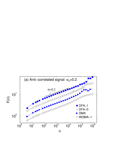
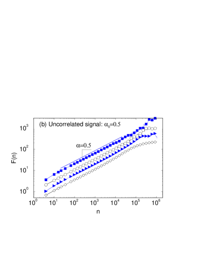
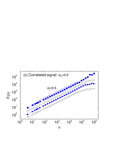
Figure 1: A comparison of the scaling behavior obtained from the DMA, WDMA-1, DFA-0, and DFA-1 methods for artificially generated power-law correlated signals with a scaling exponent $\alpha_{0}$. The length of the signals is $N=2^{20}$. Scaling curves $F(n)$ versus. scale $n$ for (a) an anti-correlated signal with $\alpha_{0}=0.2$, (b) an uncorrelated signal with $\alpha_{0}=0.5$ and (c) a positively correlated signal with $\alpha_{0}=0.8$. At small scales, all methods exhibit a weak crossover, which is more pronounced for anti-correlated signals. At large scales, the $F(n)$ curves obtained from DMA, WDMA-1, and DFA-0 exhibit a clear crossover to a flat region for all signals, independent of the type of correlations. No such crossover is observed for the scaling curves obtained from the DFA-1 method, suggesting a more accurate estimate of the scaling exponent $\alpha_{0}$ at large scales.

Figure 2: A comparison of the performance of the different scaling methods (DMA, WDMA-1, DFA-0, DFA-1, and DFA-2) when applied to artificially generated signals with long-range power-law correlations. Here $\alpha_{0}$ is the correlation exponent of the generated signals and $\alpha$ is the exponent value estimated using different methods. For all methods we obtain $\alpha$ by fitting the corresponding scaling curves $F(n)$ in the range $n\epsilon[10^{2},10^{4}]$. Flat regions indicate the limitations of the methods in accurately estimating the degree of correlations in the generated signals, as the “output” exponent $\alpha$ remains unchanged when the “input” exponent $\alpha_{0}$ is varied.

Figure 3: A comparison of the local scaling exponent $\alpha_{\rm loc}$ as a function of the scale $n$ for the DMA, WDMA-1, DFA-0, and DFA-1 methods. We consider signals of length $N=2^{20}$ and varying values of the correlation exponent $\alpha_{0}$. The local scaling exponent $\alpha_{\rm loc}$ quantifies the stability of the scaling curves $F(n)$ (see Fig. 1) and is expected to exhibit small fluctuations around a constant value $\alpha_{0}$ if $F(n)$ is well fitted by a power-law function. $\alpha_{0}$ is denoted by horizontal dotted lines. Symbols denote the estimated values of $\alpha_{\rm loc}$ and represent average results from $50$ realizations of artificial signals for each value of the “input” scaling exponent $\alpha_{0}$. Deviations from the horizontal lines at small or at large scales indicate limitations of the methods to accurately quantify the build-in correlations in different scaling ranges.

Figure 4: Values of the local scaling exponent $\alpha_{\rm loc}$ as a function of the scale $n$ obtained from 20 different realizations of artificial anti-correlated signals with an identical scaling exponent $\alpha_{0}~{}=~{}0.2$.

Figure 5: Values of the local scaling exponent $\alpha_{\rm loc}$ as a function of the scale $n$ obtained from 20 different realizations of artificial uncorrelated signals with an identical scaling exponent $\alpha_{0}=0.5$.

Figure 6: Values of the local scaling exponent $\alpha_{\rm loc}$ as a function of the scale $n$ obtained from 20 different realizations of artificial positively correlated signals with an identical scaling exponent $\alpha_{0}=0.8$.

Figure 7: Probability density of the estimated values of $\alpha_{0}-\delta<\alpha_{\rm loc}<\alpha_{0}+\delta$, where $\delta=0.02$ for a varying scale range $n$ and for different values of the “input” correlation exponent $\alpha_{0}$. Separate panels show the performance of the DMA, WDMA-1, DFA-0 and DFA-1 methods, respectively, based on 50 realizations of correlated signals for each value of $\alpha_{0}$. The probability density values $p$ are presented in color, with the darker color corresponding to higher values as indicated in the vertical columns next to each panel. A perfect scaling behavior would correspond to dark-colored columns spanning all scales $n$ for each value of $\alpha_{0}$.

Step 2: Once the moving average $\tilde{y}_{n}(i)$ is obtained, we next detrend the signal by subtracting the trend $\tilde{y}_{n}$ from the integrated profile $y(i)$

$$C_{n}(i)\equiv y(i)-\tilde{y}_{n}(i).$$ (10)

For the backward moving average, we then calculate the fluctuation for a window of size $n$ as

$$F(n)=\sqrt{\frac{1}{N-n+1}\sum_{i=n}^{N}[C_{n}(i)]^{2}}.$$ (11)

For the centered moving average the fluctuation for a window of size $n$ is calculated as

$$F(n)=\sqrt{\frac{1}{N-n+1}\sum_{i=[\frac{n+1}{2}]}^{N-[\frac{n}{2}]}[C_{n}(i)]^{2}},$$ (12)

Step 3: Repeating the calculation for different $n$, we obtain the fluctuation function $F(n)$. A power law relation between the fluctuation function $F(n)$ and the scale $n$ (see Eq.(5)) indicates a self-similar behavior.

When the moving average $\tilde{y}_{n}$ is calculated as in Eq.(6), Eq.(7), Eq.(8) and Eq.(9), we have the detrended moving method (DMA), the centered detrened moving average (CDMA), the weighted detrended moving average with order $\ell$ (WDMA-$\ell$) and the weighted centered detrended moving average (WCDMA) respectively.

III Analysis and comparison

Using the modified Fourier filtering method MFFM , we generate uncorrelated, positively correlated, and anti-correlated signals $u(i)$, where $i=1,2,...,N$ and $N=2^{20}$, with a zero mean and unit standard deviation. By introducing a designed power-law behavior in the Fourier spectrum MFFM ; zhipre2002 , the method can efficiently generate signals with long-range power-law correlations characterized by an a-priori known correlation exponent $\alpha_{0}$.

III.1 Detrended moving average method and DFA

In this section we investigate the performance of the DMA and WDMA-1 methods when applied to signals with different type and degree of correlations, and compare them to the DFA method. Specifically, we compare the features of the scaling function $F(n)$ obtained from the DMA and WDMA-1 methods with the DFA method, and how accurately these methods estimate the correlation properties of the artificially generated signals $u(i)$. Ideally, the output scaling function $F(n)$ should exhibit a power-law behavior over all scales $n$, characterized by a scaling exponent $\alpha$ which is identical to the given correlation exponent $\alpha_{0}$ of the artificial signals. Previous studies kunpre2001 ; zhipre2002 ; zhipre2004 show that the scaling behavior obtained from the DFA method depends on the scale $n$ and the order $\ell$ of the polynomial fit when detrending the signal. We investigate if the results of the DMA and WDMA-1 method also have a similar dependence on the scale $n$. We also show how the scaling results depend on the order $\ell$ when using WDMA-$\ell$ with $\ell=2,3,4,5$ are applied to the signals (See Appendix I).

To compare the performance of different methods, we first study the behavior of the scaling function $F(n)$ obtained from DFA-0, DFA-1, DMA, and WDMA-1. In Fig. 1 we show the rms fluctuation function $F(n)$ obtained from the different methods for an anti-correlated signal with correlation exponent $\alpha_{0}=0.2$, an uncorrelated signal with $\alpha_{0}=0.5$, and a positively correlated signal with $\alpha_{0}=0.8$. We find that in the intermediate regime $F(n)$ (obtained from all methods) exhibits an approximate power-law behavior characterized by a single scaling exponent $\alpha$. At large scales $n$ for DFA-0, DMA, and WDMA-1, we observe a crossover in $F(n)$ leading to a flat regime. With increasing $\alpha_{0}$ this crossover becomes more pronounced and moves to the intermediate scaling range. In contrast, such a crossover at large scales is not observed for DFA-1, indicating that the DFA-1 method can better quantify the correlation properties at large scales. At small scales $n$ the scaling curves $F(n)$ obtained from all methods exhibit a crossover which is more pronounced for anti-correlated signals ($\alpha_{0}=0.2$) and becomes less pronounced for uncorrelated ($\alpha_{0}=0.5$) and positively correlated signals ($\alpha_{0}=0.8$).

We next systematically examine the performance of the DFA-0, DFA-1, DMA and WDMA-1 methods by varying $\alpha_{0}$ over a very broad range of values ($0.1\leq\alpha_{0}\leq 3.5$) [Fig. 2]. For all four methods, we compare $\alpha_{0}$ with the exponent $\alpha$ obtained from fitting the rms fluctuation function $F(n)$ in the scaling range $10^{2}<n<10^{4}$, i.e., the range where all methods perform well according to our observations in Fig. 1. If the methods work properly, for each value of the “input” exponent $\alpha_{0}$ we expect the estimated “output” exponent to be $\alpha=\alpha_{0}$. We find that the scaling exponent $\alpha$, obtained from different methods, saturates as the “input” correlation exponent $\alpha_{0}$ increases, indicating the limitation of each method. The saturation of scaling exponent at $\alpha=1$ indicates that DMA and WDMA-1 do not accurately quantify the correlation properties of signals with $\alpha_{0}>1$.

In contrast, the DFA-$\ell$ method can quantify accurately the scaling behavior of strongly correlated signals if the appropriate order $\ell$ of the polynomial fit is used in the detrending procedure. Specifically, we find that the values of the scaling exponent $\alpha$ obtained from the DFA-$\ell$ are limited to $\alpha\leq\ell+1$. Thus the DFA-$\ell$ can quantify the correlation properties of signals characterized by exponent $\alpha_{0}\leq\ell+1$. For signals with $\alpha_{0}>\ell+1$ we find that the output exponent $\alpha$ from the DFA-$\ell$ method remains constant at $\alpha=\ell+1$. These findings suggest that in order to obtain a reliable estimate of the correlations in a signal one has to apply the DFA-$\ell$ for several increasing orders $\ell$ until the obtained scaling exponent $\alpha$ stops changing with increasing $\ell$.

Since the accuracy of the scaling exponent obtained from the different methods depends on the range of scales $n$ over which we fit the rms fluctuation function $F(n)$ (as seen in Fig. 1), and since different methods exhibit different limitations for the range of scaling exponent values (as demonstrated in Fig. 2), we next investigate the local scaling behavior of the $F(n)$ curves to quantify the performance of the different methods in greater details. To ensure a good estimation of the local scaling behavior, we calculate $F(n)$ at scales $n=4\times 2^{i/64}$, $i=0,1,2,...$, which in log scale provides $64$ equidistant points for $F(n)$ per bin of size $\log{2}$. To estimate the local scaling exponent $\alpha_{\rm loc}$, we locally fit $F(n)$ in a window of size $w=3\log{2}$, e.g, $\alpha_{\rm loc}$ is the slope of $F(n)$ in a window containing $3\times 64$ points. To quantify the detailed features of the scaling curve $F(n)$ at different scales $n$, we slide the window $w$ in small steps of size $\Delta=\frac{1}{4}\log{2}$ starting at $n=4$, thus obtaining approximately $70$ equidistant $\alpha_{\rm loc}$ in log scale per each scaling curve. We consider the average value of $\alpha_{\rm loc}$ obtained from $50$ different realizations of signals with the same correlation exponent $\alpha_{0}$.

In Fig. 3, we compare the behavior of $\alpha_{\rm loc}$ as a function of the scale $n$ to more accurately determine the best fitting range in the scaling curves $F(n)$ obtained from the DMA, WDMA-1, DFA-0, and DFA-1. A rms fluctuation function exhibiting a perfect scaling behavior would be characterized by $\alpha_{\rm loc}=\alpha_{0}$ for all scales $n$ and for all values of $\alpha_{0}$ denoted by horizontal lines in Fig. 3. A deviation of the $\alpha_{\rm loc}$ curves from these horizontal lines indicates an inaccuracy in quantifying the correlation properties of a signal and the limitation of the methods. Our results show that the performance of different methods depends on the “input” $\alpha_{0}$ and scale $n$. At small scales and for $\alpha_{0}<0.8$ we observe that $\alpha_{\rm loc}$ for all methods deviates up from the horizontal lines suggesting an overestimation of the real correlation exponent $\alpha_{0}$. This effect is less pronounced for uncorrelated and positively correlated signals. At intermediate scales $\alpha_{\rm loc}$ exhibits a horizontal plateau indicating that all methods closely reproduce the input exponent for $\alpha_{0}<0.8$. This intermediate scaling regime changes for different types of correlations and for different methods. At large scales of $n>10^{4}$, the DMA, WDMA-1, and DFA-0 methods strongly underestimate the actual correlations in the signal, with $\alpha_{\rm loc}$ curves sharply dropping for all values of $\alpha_{0}$ [Fig. 3(a),(b),(c)]. In contrast, the DFA-1 method accurately reproduces $\alpha_{0}$ at large scales with $\alpha_{\rm loc}$ following the horizontal lines up to approximately $N/10$ [Fig. 3(d)]. In addition, the DFA-1 method accurately reproduces the correlation exponent at small and intermediate scales even when $\alpha_{0}>1$ [Fig. 3(d)], while the DMA, WDMA-1 and DFA-0 are limited to $\alpha_{0}<0.8$.

For a certain “input” correlation exponent $\alpha_{0}$, we can estimate the good fitting regime of $F(n)$ to be the length of the plateau in Fig. 3. For example, for $\alpha_{0}=0.2$ the calculated scaling exponent $\alpha_{loc}$ obtained from the DMA method is approximately equal to the expected value $\alpha_{0}=0.2$ within a range of two decades ($10^{2}<n<10^{4}$). Similarly, the good fitting range of $F(n)$ obtained from the DFA-0 for $\alpha_{0}=0.2$ is about three decades ($10^{2}<n<10^{5}$). However, the calculated local scaling exponent $\alpha_{loc}$ can fluctuate for different realizations of correlated signals. Although the mean value obtained from many independent realizations is close to the expected value, the fluctuation of the estimated scaling exponent can be very large. Thus, it is possible for $\alpha_{loc}$ to deviate from $\alpha_{0}$ and the scaling range estimated from Fig. 3 may not be a good fitting range. Therefore, it is necessary to study the dispersion of the local scaling exponent to determine the reliability of the “good” fitting range estimated from Fig. 3. In Fig. 4, 5, 6 we show the results for $\alpha_{\rm loc}$ from 20 different realizations of the correlated signal with $\alpha_{0}=0.2$, $\alpha_{0}=0.5$, and $\alpha_{0}=0.8$ respectively. For all methods, we observe that there is a large dispersion of $\alpha_{\rm loc}$, indicating strong fluctuations in the scaling function $F(n)$ at large scales $n$ ($n\sim 10^{3}$ for DMA and WDMA-1 and $n\sim 10^{4}$ for DFA-0 and DFA-1) [Fig. 4, 5, 6]. This suggests that the good fitting range obtained only from the mean value of $\alpha_{loc}$, as shown in Fig. 3, may be overestimated.

To better quantify the best fitting range for different methods and for different types of correlations we develop a three-dimensional representation [Fig. 7]. Based on 50 realizations of correlated signals with different values of $0.1<\alpha_{0}<1.1$, for each scale $n$ we define the probability $p$ (normalized frequency) to obtain values for $\alpha_{0}-\delta<\alpha_{\rm loc}<\alpha_{0}+\delta$, where $\delta=0.02$ (arguments supporting this choice of $\delta$ are presented in section III(B)). Again, as in Fig. 3, for each realization of correlated signals with a given $\alpha_{0}$, we calculate $\alpha_{\rm loc}$ by fitting the rms fluctuation function $F(n)$ in a window of size $w=3\log{2}$ sliding in steps of $\Delta=\frac{1}{4}\log{2}$. Vertical color bars in Fig. 7 represent the value of the probability $p$ — darker colors corresponding to higher probability to obtain accurate values for $\alpha_{loc}$. Thus dark-colored columns in the panels of Fig. 7 represent the range of scales $n$ where the methods perform best.

For the DMA and WDMA-1 methods, we find that with high probability $(p>0.7)$, accurate scaling results can be obtained in the scaling range of two decades for $0.4\leq\alpha_{0}\leq 0.6$. However, WDMA-1 performs better at small scales compared to DMA. For explanation why the WDMA-1 performs better at small scales compared to DMA, see Appendix II. In contrast, DFA-0 exhibits an increased fitting range of about three decades for $0.4\leq\alpha_{0}\leq 0.8$, while for the DFA-1 we find the best fitting range to be around three decades for $\alpha_{0}>0.5$. For strongly anti-correlated signals ($\alpha_{0}<0.2$), all methods do not provide an accurate estimate of the scaling exponents $\alpha_{0}$. However, by integrating anti-correlated signals with $\alpha_{0}<0.3$ and applying the DFA-1 method, we can reliably quantify the scaling exponent, since DFA-1 has the advantage to quantify signals with $\alpha_{0}>1$ [Fig. 7(d)]. This can not be obtained by the other three methods [Fig. 7(a),(b),(c)].

Figure 8: A comparison of the local scaling exponent $\alpha_{\rm loc}$ as a function of the scale $n$ for the DMA, CDMA, DFA-0, and DFA-1 methods. We consider signals of length $N=2^{20}$ and varying values of the correlation exponent $\alpha_{0}$. The local scaling exponent $\alpha_{\rm loc}$ quantifies the stability of the scaling curves $F(n)$ and is expected to exhibit small fluctuations around a constant value $\alpha_{0}$ if $F(n)$ is well fitted by a power-law function. $\alpha_{0}$ is denoted by horizontal dotted lines. Symbols denote the estimated values of $\alpha_{\rm loc}$ and represent average results from $50$ realizations of artificial signals for each value of the “input” scaling exponent $\alpha_{0}$. Deviations from the horizontal lines at small or at large scales indicate limitations of the methods to accurately quantifying the build-in correlations in different scaling ranges. Error bars represent the standard deviation for each average value of $\alpha_{loc}$ at different scales $n$, and determine the accuracy of each method.

III.2 Centered moving average method and DFA

Figure 9: Probability density of the estimated values of $\alpha_{0}-\delta<\alpha_{\rm loc}<\alpha_{0}+\delta$, where $\delta=0.02$ for a varying scale range $n$ and for different values of the “input” correlation exponent $\alpha_{0}$. The two panels show the performance of the DMA and CDMA methods, respectively, based on 50 realizations of correlated signals for each value of $\alpha_{0}$. The probability density values $p$ are presented in color, with the darker color corresponding to higher values, as indicated in the vertical columns next to each panel. A perfect scaling behavior would correspond to dark-colored columns spanning all scales $n$ for each value of $\alpha_{0}$.

Figure 10: Local scaling exponent $\alpha_{\rm loc}$ as a function of the scale $n$ for the WCDMA method. We consider signals of length $N=2^{20}$ and varying values of the correlation exponent $\alpha_{0}$. The expected value of the exponent $\alpha_{0}$ is denoted by horizontal dotted lines. Symbols denote the estimated values of $\alpha_{\rm loc}$ and represent average results from $50$ realizations of artificial signals for each value of the “input” scaling exponent $\alpha_{0}$. Deviations from the horizontal lines at small or at large scales indicate limitations of the methods to accurately quantify the build-in correlations in different scaling ranges. Error bars represent the standard deviation for each average value of $\alpha_{loc}$ at different scales $n$, and determine the accuracy of the method.

Figure 11: A comparison of the local scaling exponent $\alpha_{\rm loc}$ as a function of the scale $n$ obtained from (a) the WCDMA method and (b) the DFA-1 method. Symbols denote the estimated values of $\alpha_{\rm loc}$ calculated as in Fig.10 for different “input” scaling exponents $\alpha_{0}>1$. Error bars representing the standard deviation around the average $\alpha_{loc}$ are smaller for the DFA-1 method at all scales $n$, indicating that the DFA-1 method provides more reliable results.

Figure 12: Probability density of estimated values of $\alpha_{0}-\delta<\alpha_{\rm loc}<\alpha_{0}+\delta$, where $\delta=0.01$ for varying scale range $n$ and for different values of the “input” correlation exponent $\alpha_{0}$. The two panels show the performance of the DMA and DFA-1 methods, respectively, based on 50 realizations of correlated signals for each value of $\alpha_{0}$. The probability density values $p$ are presented in color, with darker color corresponding to higher values as indicated in the vertical columns next to each panel. A perfect scaling behavior would correspond to dark-colored columns spanning all scales $n$ for each value of $\alpha_{0}$.

Figure 13: A comparison of the local scaling exponent $\alpha_{\rm loc}$ as a function of the scale $n$ for the WDMA-$\ell$ method with different order $\ell=2,...,5$ of the weighted moving average. We consider signals of length $N=2^{20}$ and varying values of the correlation exponent $\alpha_{0}$. The local scaling exponent $\alpha_{\rm loc}$ quantifies the stability of the scaling curves $F(n)$ (see Fig. 1), and is expected to exhibit small fluctuations around a constant value $\alpha_{0}$ if $F(n)$ is well fitted by a power-law function. $\alpha_{0}$ is denoted by horizontal dotted lines. Symbols denote the estimated values of $\alpha_{\rm loc}$ and represent average results from $50$ realizations of artificial signals for each value of the “input” scaling exponent $\alpha_{0}$. For small values of $\ell$ at small and intermediate scales $n$, WDMA-$\ell$ accurately reproduces the scaling behavior of signals with $0.4<\alpha_{0}<0.8$, while for large $\ell$ , the scaling behavior of anti-correlated signals with $\alpha_{0}<0.4$ are better reproduced at small scales.

Figure 14: Probability density of estimated values of $\alpha_{0}-\delta<\alpha_{\rm loc}<\alpha_{0}+\delta$, where $\delta=0.02$ for the varying scale range $n$ and for different values of the “input” correlation exponent $\alpha_{0}$. Separate panels show the performance of the WDMA-2, WDMA-3, WDMA-4, and WDMA-5 methods, respectively, based on 50 realizations of correlated signals for each value of $\alpha_{0}$. The probability density values $p$ are presented in color, with the darker color corresponding to higher values, as indicated in the vertical columns next to each panel. A perfect scaling behavior would correspond to dark-colored columns spanning all scales $n$ for each value of $\alpha_{0}$.

To test the accuracy of the CDMA method we perform the same procedure as shown in Fig.3. We calculate the local scaling exponent $\alpha_{loc}$ for signals with different “input” correlation exponent $\alpha_{0}$ and for a broad range of scales $n$ [Fig.8]. We find that for $0.3<\alpha_{0}<0.8$ the CDMA method performs better than the DMA for all scales $n$, and the average value of $\alpha_{loc}$ follows very closely the expected values of $\alpha$ indicated by horizontal lines in Fig.8. For anti-correlated signals with $\alpha_{0}\leq 0.3$, both DMA and CDMA overestimate the value of $\alpha_{0}$ at small scales $n<10^{2}$. For strongly correlated signals with $\alpha_{0}>0.8$, CDMA underestimates $\alpha_{0}$ at small scales $n<10^{2}$, in contrast to DMA which overestimates $\alpha_{0}$. For correlated signals with $\alpha_{0}>1.1$ (not shown in Fig.8(c)) the deviation of $\alpha_{loc}$ from the expected value $\alpha_{0}$ for the CDMA method becomes even more pronounced and spreads to large scales. At intermediate and large scales CDMA performs much better — $\alpha_{loc}$ closely follows the horizontal lines [Fig.8 (a),(c)]. These differences in the performance of the DMA and CDMA methods are also clearly seen in the probability density plots shown in Fig.9.

Next, we compare the stability of the DMA, CDMA, DFA-0, and DFA-1 methods in reproducing the same “input” value of $\alpha_{0}$ for different realizations of correlated signals. We generate 50 realizations of signals for each $\alpha_{0}$, and we obtain the average value and the standard deviation of $\alpha_{loc}$ for a range of scales $n$. The values of the standard deviation are represented by error bars in Fig.8 for each value of $\alpha_{loc}$ at all scales $n$. We find that with increasing scales $n$, the standard deviation gradually increases, and that for DMA the standard deviation is less than $0.02$ while for DFA the standard deviation is less than $0.01$ in the range of scales $n$ up to $N/100$ ($N$ is the signal length). For all methods at scales $n>N/100$, the standard deviation increases more rapidly, and thus the stability of the methods in reproducing the same value of the exponent for different realizations decreases.

In Fig.10 we present the dependence of $\alpha_{loc}$ on the scale $n$ for the weighted centered detrended moving average method. Compared to the CDMA method, the WCDMA method weakens the overestimation of $\alpha_{loc}$ at small scale for anti-correlated signals and provides accurate results of $\alpha_{loc}$ at small scales for positively correlated signals with $0.5<\alpha_{0}<1$. Compared to the DFA method, the WCDMA performs better at small scales for $0.5<\alpha_{0}<1.0$. However, at larger scales $n>10^{2}$, the standard deviation of DFA-1 is smaller than that of WCDMA (Figs.8(d), 10 and 11), indicating more reliable results for the local scaling exponent $\alpha_{loc}$ obtained from DFA-1.

Finally, we test how the choice of the parameter $\delta$ will affect the probability density plots shown in Fig.7 and Fig.9. To access the precision of the methods one has to increase the confidence level by decreasing $\delta$. In Fig.7 and Fig.9 we have chosen $\delta=0.02$ to correspond to the value of the standard deviation for $\alpha_{loc}$ at scales $n<10^{4}$ as estimated by the DMA method [Fig.8]. We demonstrate that the distribution plot for DMA with $\delta=0.02$ (shown in Fig.7) changes dramatically when we chose $\delta=0.01$ (as shown in Fig.12(b)). This result confirms the observation from Fig.8(a) and (d) that the DFA-1 method is more stable (smaller standard deviation) and more accurate (average of $\alpha_{loc}$ closer to the theoretically expected value $\alpha_{0}$) than the DMA method.

IV discussion

We have systematically studied the performance of the different variants of DMA method when applied to signals with long-range power-law correlations, and we have compared them to the DFA method. Specially, we have considered two categories of detrended moving average methods — the simple moving average and the weighted moving average — in order to investigate the effect of the relative contribution of data points included in the moving average window when estimating correlations in signals. To investigate the role of “past” and “future” data points in the dynamic averaging process for signals with different correlations, we have also considered the cases of backward and centered moving average within each of the above two categories. Finally, we have introduced a three-dimensional representation to compare the performance of different variants of the DMA method and the DFA methods over different scaling ranges based on an ensemble of multiple signal realizations.

We find that the simple backward moving average DMA method and the weighted backward moving average method WDMA-$\ell$ have limitations when applied to signals with very strong correlations characterized by scaling exponent $\alpha_{0}>0.8$. A similar limitation is also found for the $\ell=0$ order of the DFA method. However, for higher order $\ell$, the DFA-$\ell$ method can accurately quantify correlations with $\alpha_{0}<{\ell}+1$. We also find that at large scales the DMA, WDMA-$\ell$, and DFA-0 methods underestimate the correlations in signals with $0.5<\alpha_{0}<1.0$, while the DFA-$\ell$ method can more accurately quantify the scaling behavior of such signals. Further, we find that the scaling curves obtained from the DFA-1 method are stable over a much broader range of scales compared to the DMA, WDMA-1, and DFA-0 methods, indicating a better fitting range to quantify the correlation exponent $\alpha_{0}$. In contrast, we find that WDMA-$\ell$ with a higher order $\ell$, more accurately reproduce the correlation properties of anti-correlated signals ($\alpha_{0}<0.5$) at small scales. Accurate results for anti-correlated signals can also be obtained from the DFA-1 method after first integrating the signal and thus reducing the value of the estimated correlation exponent by 1.

In contrast to the simple backward moving average (DMA) and DFA-0 methods, the centered moving average CDMA provides a more accurate estimate of the correlations in signals with $0.3<\alpha_{0}<0.7$ at small scales $n<10^{2}$, and in signals with $\alpha_{0}>0.7$ at intermediate scales $10^{2}<n<10^{4}$. However, the CDMA method strongly underestimates correlations in signals with $\alpha_{0}>0.7$ at small scales $(n<10^{2})$, while the DFA-1 method reproduces quite accurately the correlations of signals with $\alpha_{0}>0.7$ at both small and intermediate scales. We also find that by introducing weighted centered moving average WCDMA, one can overcome the limitation of the CDMA method in estimating correlations in signals with $\alpha_{0}>0.5$ at small scales $(n<10^{2})$. On the other hand, the WCDMA method is characterized by larger error bars for $\alpha_{loc}$ at intermediate scales compared to the CDMA method. Further, we find that the performance of the WCDMA is comparable to the DFA-1 method for signals with $0.5<\alpha_{0}<1$. At small scales the WCDMA performs better than the DFA-1 method, while at the intermediate scales $10^{2}<n<10^{4}$, DFA-1 provides more reliable local scaling exponent with smaller standard deviation based on 50 independent realizations for each $\alpha_{0}$. For very strongly correlated signals with $\alpha_{0}>1$, we find that the DFA-1 method performs much better at all scales compared to WCDMA and all other variants of the DMA method.

V APPENDIX I

Higer order weighted moving average

To account for different types of correlations in signals, we consider the $\ell$-order weighted moving average (WDMA-$\ell$), defined as

$$\tilde{y}_{n}(i)\equiv\frac{(1-\lambda)}{\ell}\sum_{k=0}^{{\ell}-1}y(i-k)+\lambda\tilde{y}_{n}(i-{\ell}),$$ (13)

where $\lambda=n/(n+\ell)$, $\ell$ is the order of the moving average, $y(i)$ is defined in Eq.(1). The relative importance of the two terms entering the function in Eq.(13), can be further understood by analyzing the properties of the transfer function $H(f)$ in the frequency domain (see Appendix II).

Compared to the traditional exponentially weighted moving average (of order $\ell=1$ ) where the terms in Eq.(13) decrease exponentially, the higher order $\ell>1$ allows for a slower, step-size decrease of the terms in Eq.(13) with a “step” of size $\ell$. The fluctuation function $F(n)$ is obtained following Eq.(10) and Eq.(11). The WDMA-$\ell$ allows for a more gradual decrease in the distribution of weights in the moving average box, and thus may be more appropriate when estimating the scaling behavior of anti-correlated and uncorrelated signals.

We apply the WDMA-$\ell$ method for increasing values of $\ell$ to correlated signals with varied values of the scaling exponent $\alpha_{0}$. To study the performance of the WDMA-$\ell$ methods, we estimate the scaling behavior of the rms fluctuation function $F(n)$ at different scales $n$ by calculating the local scaling exponent $\alpha_{\rm loc}$ in the same way as discussed in Fig. 3. We find that at large scales for $\ell=2,...,5$, the $\alpha_{\rm loc}$ curves deviate significantly from the expected values $\alpha_{0}$ — presented with horizontal dashed lines in Fig. 13. This indicates that the WDMA-$\ell$ method significantly underestimates the strength of the correlations in our artificially generated signals. Further, as for $\ell=1$, we find that for higher order $\ell>1$ the WDMA-$\ell$ methods exhibit an inherent limitation to accurately quantify the scaling behavior of positively correlated signals with $\alpha_{0}>0.7$. This behavior is also clear from our three-dimensional presentation in Fig. 14. For anti-correlated signals, however, the WDMA-$\ell$ performs better at small and intermediate scales for increasing order $\ell$ as $\alpha_{0}$ decreases [Fig. 13] (see Appendix II). These observations are also confirmed from the three-dimensional probability histograms in Fig. 14, where it is clear that the scaling range for the best fit shrinks for positively correlated signals $(\alpha_{0}>0.5$) for increasing order $\ell$, while for anti-correlated signals $(\alpha_{0}<0.5)$, there is a broader range of scales over which a best fit (with a probability of $p>0.7$) is observed.

VI APPENDIX II

Moving average methods in frequency domain

Figure 15: Plot of the moving average filter kernel in the time (a) and in the frequency domain (b) respectively.

Figure 16: Plot of the function $|H(f)|^{2}$ for the simple moving average with $n=4$, $|H_{4}(f)|^{2}$; for the weighted moving average, with $n=4$ and $\ell=2$, $|H_{4,2}(f)|^{2}$ respectively ; for the weighted moving average with $n=4$ and $\ell=4$ $|H_{4,4}(f)|^{2}$ respectively.

In this appendix, the performance of the DMA algorithm is discussed in the frequency domain. The interest of the frequency domain derives from the simplification designed to describe the effect of the detrending function $\tilde{y}_{n}(i)$ in terms of the product of the square modulus of the transfer function $H_{n}(f)$ and of $S(f)$, the power spectral density of the noisy signal $y(i)$.

The simple moving average $\tilde{y}_{n}(i)$ of window size $n$ is defined as

$$\tilde{y}_{n}(i)\equiv\frac{1}{n}\sum_{k=0}^{n-1}y(i-k)\hskip 5.0pt,$$ (14)

corresponding to the discrete form of the causal convolution integral, where the convolution kernel introduces the memory effect. Eq.(14) is a sum with a constant memory kernel $h(t)$, i.e., a step function with an amplitude $1/n$ [Fig.15(a)]. The function $h(t)$ uniformly weights the contribution of all the past events in the window $[0,n)$, thus it works better for random paths with a correlation exponent centered around $0.5$. For higher degrees of correlation/anti-correlation, it should be taken into account (as already explained in the section describing the DMA function) that each data point is more correlated to the most recent points than to the points further away.

In the frequency domain, $\tilde{y}_{n}(i)$ is characterized by the transfer function $H_{n}(f)$ (the Dirichlet kernel), which is

$$H_{n}(f)=\frac{\sin(n\pi f)}{n\pi f}\cdot e^{-in\pi f}.$$ (15)

$H_{n}(f)$ takes the values $H_{n}(0)=1$ and $H_{n}(kf_{0})=0$ for $k=1,2,...n$.

The transfer function $H(f)$ of any filter should ideally be a window of constant amplitude, going to zero very quickly above the cut-off frequency $1/n$. By observing the curves of Fig.15(b) and Fig.16, it is clear that the filtering performance of $H_{n}(f)$ is affected by the presence of the side lobes at frequency higher than $1/n$.

As observed in Fig.16, $|H_{4}(f)|^{2}$ presents a side lobe allowing the components of the signal $y(i)$, with a frequency between $1/n$ and $2/n$ (i.e., time scales between $n/2$ and $n$) to pass through the filter, thus giving a spurious contribution to $\tilde{y}_{n}(i)$. These components contribute to the rms $F(n)$ (defined in Eq.(11)) less than what should correspond to $n$ on the basis of the scaling law $F(n)\sim n^{\alpha}$ , with the consequence of increasing the slope $F(n)$ at small scales.

We next discuss the reasons why the weighted moving average might reduce this effect. The exponentially weighted moving average (WDMA-$\ell$) weights recent data more than older data. It is defined as

$$\tilde{y}_{n,\ell}(i)\equiv\frac{(1-\lambda)}{\ell}\sum_{k=0}^{\ell-1}y(i-k)+\lambda\tilde{y}_{n,\ell}(i-\ell)\hskip 8.0pt.$$ (16)

The coefficients are commonly indicated as weights of the filter and are given by

$$\lambda=\frac{n}{\ell+n}\hskip 8.0pt.$$ (17)

Taking the Fourier transform on Eq. (16), we obtain

$$\tilde{Y}_{n,\ell}(f)=(1-\lambda)H_{\ell}(f)\cdot Y(f)+\lambda\tilde{Y}_{n,\ell}(f)\cdot e^{-i2\pi\ell f},$$ (18)

where $Y(f)$, $\tilde{Y}_{n,\ell}(f)$ are the Fourier transforms of $y(i)$ and $\tilde{y}_{n,\ell}(i)$ respectively. Further, we have

$$\tilde{Y}_{n,\ell}(f)=\frac{1-\lambda}{1-\lambda e^{-i2\pi\ell f}}\cdot H_{\ell}(f)\cdot Y(f).$$ (19)

Thus the transfer function is

$$H_{n,\ell}(f)=\frac{1-\lambda}{1-\lambda e^{-i2\pi\ell f}}\cdot H_{\ell}(f).$$ (20)

From Eq.(20), one can find that the cutoff frequency for $|H_{n,\ell}(f)|^{2}$ is $min$[$1/(2\pi\sqrt{n(n+\ell)}),1/\ell$]. In Fig. 16, the transfer function of the weighted moving averages with $n=4$ and $\ell=2$ and with $n=4$ and $\ell=4$ respectively are shown. It can be observed that the effect of the side lobe to the performance of $|H_{4,2}(f)|^{2}$ and $|H_{4,4}(f)|^{2}$ has become negligible compared to that of $|H_{4}(f)|^{2}$ , with the consequence of reducing the high frequency components in the detrended signal and thus reducing the deviation of the $\alpha_{\rm loc}$, as discussed in the paper.

References

- (1) P. A. Robinson,Phys. Rev. E 67, 032902 (2003).
- (2) K. Ivanova, T. P. Ackerman, E. E. Clothiaux, P. Ch. Ivanov, H. E. Stanley, and M. Ausloos, J. Geophys. Res. 108,4268 (2003).
- (3) Z. Siwy, M. Ausloos, and K. Ivanova, Phys. Rev. E 65, 031907 (2002).
- (4) P. A. Varotsos, N. V. Sarlis, and E. S. Skordas, Phys. Rev. E 67, 021109 (2003).
- (5) P. A. Varotsos, N. V. Sarlis, and E. S. Skordas, Phys. Rev. E 68, 031106 (2003).
- (6) E. Koscielny-Bunde, A. Bunde, S. Havlin, H. E. Roman, Y. Goldreich, and H. J. Schellnhuber, Phys. Rev. Lett. 81, 729 (1998).
- (7) P. Talkner and R. O. Weber, Phys. Rev. E 62, 150 (2000).
- (8) J. F. Eichner, E. Koscielny-Bunde, A. Bunde, S. Havlin, and H. J. Schellnhuber, Phys. Rev. E 68, 046133 (2003).
- (9) K. Fraedrich and R. Blender, Phys. Rev. Lett. 90, 108501 (2003).
- (10) M. Pattantyus-Abraham, A. Kiraly, and I. M. Janosi, Phys. Rev. E69, 021110 (2004).
- (11) A. Montanari, R. Rosso, and M. S. Taqqu, Water Resour. Res, 36, (5) 1249 (2000).
- (12) C. Matsoukas, S. Islam, and I. Rodriguez-Iturbe,J. Geophys. Res, [Atmos.] 105, 29165 (2000).
- (13) M. A. Moret, G. F. Zebende, E. Nogueira, and M. G. Pereira, Phy. Rev. E 68, 041104 (2003).
- (14) R.G. Kavasseri, R. Nagarajan, IEEE Trans.Cir.Sys. 51(11), 2255 (2004).
- (15) G.F. Zebende, M.V.S. da Silva, A.C.P. Rosa, A.S. Alves, J.C.O. de Jesus, M.A. Moret, Physca A 342, 322 (2004).
- (16) C. -K. Peng, S. V. Buldyrev, S. Havlin, M. Simons, H. E. Stanley, and A. L. Goldberger, Phys. Rev. E 49, 1685 (1994).
- (17) S. V. Buldyrev, A. L. Goldberger, S. Havlin, C.-K. Peng, H. E. Stanley, and M. Simons, Biophys. J. 65, 2673 (1993).
- (18) R. N. Mantegna, S. V. Buldyrev, A. L. Goldberger, S. Havlin, C.-K. Peng, M. Simons, and H. E. Stanley, Phys. Rev. Lett. 76, 1979 (1996).
- (19) P. Carpena, P. Bernaola–Galván, P. Ch. Ivanov, and H. E. Stanley, Nature (London) 418, 955 (2002).
- (20) N. Iyengar, C. -K. Peng, R. Morin, A. L. Goldberger, and L. A. Lipsitz, Am. J. Physiol. 40, R1078 (1996).
- (21) P. Ch. Ivanov, A. Bunde, L. A. Nunes Amaral, S. Havlin, J. Fritsch-Yelle, R. M. Baevsky, H. E. Stanley, and A. L. Goldberger, Europhys. Lett. 48, 594 (1999).
- (22) S. M. Pikkujamsa, T. H. Makikallio, L. B. Sourander, I. J. Raiha, P. Puukka, J. Skytta, C.-K. Peng, A. L. Goldberger, and H. V. Huikuri, Circulation 100, 393 (1999).
- (23) C. -K. Peng, S. Havlin, H. E. Stanley, and A. L. Goldberger, Chaos 5, 82 (1995).
- (24) D. Toweill, K. Sonnenthal, B. Kimberly, S. Lai, and B. Goldstein, Crit. Care Med. 28, 2051 (2000).
- (25) A. Bunde, S. Havlin, J. W. Kantelhardt, T. Penzel, J. H. Peter, and K. Voigt, Phys. Rev. Lett. 85, 3736 (2000).
- (26) Y. Ashkenazy, P. Ch. Ivanov, S. Havlin, C.-K. Peng, A. L. Goldberger, and H. E. Stanley, Phys. Rev. Lett. 86, 1900 (2001).
- (27) P. Ch. Ivanov, L. A. Nunes Amaral, A. L. Goldberger, M. G. Rosenblum, H. E. Stanley, and Z. R. Struzik, Chaos 11, 641 (2001).
- (28) M. Cernelc, B. Suki, B. Reinmann, Graham L. Hall, and Urs Frey , J. Appl. Physiol. 92, 1817 (2002).
- (29) J. W. Kantelhardt, Y. Ashkenazy, P. Ch. Ivanov, A. Bunde, S. Havlin, T. Penzel, J.-H. Peter, and H. E. Stanley, Phys. Rev. E 65, 051908 (2002).
- (30) R. Karasik, N. Sapir, Y. Ashkenazy, P. Ch. Ivanov, I. Dvir, P. Lavie, and S. Havlin, Phys. Rev. E 66, 062902 (2002).
- (31) J. C. Echeverria, M. S. Woolfson, J. A. Crowe, B. R. Hayes-Gill, G. D. H. Croaker, and H. Vyas, Chaos 13, 467 (2003).
- (32) K. Hu, P. Ch. Ivanov, Z. Chen, M. F. Hilton, H. E. Stanley, and S. A. Shea, Physica A 337, 307 (2004).
- (33) D. N. Baldwin, B. Suki, J. J. Pillow, H. L. Roiha, S. Minocchieri, and U. Frey, J. Appl. Physiol. 97, 1830 (2004).
- (34) J. W. Kantelhardt, S. Havlin, and P. Ch. Ivanov, Europhys. Lett. 62, 147 (2003).
- (35) R.C. Hwa, T.C. Ferree, Physica A, 338, 246 (2004).
- (36) N. Vandewalle and M. Ausloos, Phy. Rev. E 58, 6832 (1998).
- (37) Y. Liu, P. Gopikrishnan, P. Cizeau, M. Meyer, C. -K. Peng, and H. E. Stanley, Phys. Rev. E 60, 1390 (1999).
- (38) I. M. Janosi, B. Janecsko, and I. Kondor, Physica A 269, 111 (1999).
- (39) M. Ausloos, N. Vandewalle, P. Boveroux, A. Minguet, and K. Ivanova, Physica A 274, 229 (1999).
- (40) M. Roberto, E. Scalas, G. Cuniberti, and M. Riani, Physica A 269, 148 (1999).
- (41) P. Grau-Carles, Physica A 287, 396 (2000).
- (42) M. Ausloos and K. Ivanova, Phys. Rev. E 63, 047201 (2001).
- (43) P. Ch. Ivanov, A. Yuen, B. Podobnik, and Y. Lee, Phys. Rev. E 69, 056107 (2004).
- (44) K. Hu, P. Ch. Ivanov, Z. Chen, P. Carpena and H.E. Stanley, Phys. Rev. E 64, 011114 (2001).
- (45) Z. Chen, P. Ch. Ivanov, K. Hu, and H. E. Stanley, Phys. Rev. E 65, 041107 (2002).
- (46) Z. Chen, K. Hu, P. Carpena, P. Bernaola, H. E. Stanley, and P. Ch. Ivanov, Phys. Rev. E 71, 011104 (2005).
- (47) P.S. Wilson, A.C. Tomsett, R. Toumi, Phys. Rev. E 68, 017103 (2003).
- (48) R. L. Stratonovich, Topics in the Theory of Random Noise Vol. 1 (Gordon & Breach, New York, 1981).
- (49) H. E. Hurst, Trans. Am. Soc. Civ. Eng. 116, 770 (1951).
- (50) B. B. Mandelbrot and J. R. Wallis, Water Resources Res. 5, No. 2, 321 (1969).
- (51) M. S. Taqqu, V. Teverovsky, and W. Willinger, Fractals 3, 785 (1995).
- (52) E. Alessio, A. Carbone, G. Castelli, and V. Frappietro, Eur. Phys. Jour. B 27, 197 (2002).
- (53) A. Carbone, G. Castelli, and H. E. Stanley, Phys. Rev. E 69, 026105(2004).
- (54) A. Carbone and H. E. Stanley,Noise in Complex Systems and Stochastic Dynamics (Proceedings of SPIE), 5471, 45 (2004).
- (55) A. Carbone, G. Castelli and H. E. Stanley, Physica A 340, 540 (2004).
- (56) A. Carbone and H. E. Stanley, Physica A 344, 267 (2004).
- (57) H. A. Makse, S. Havlin, M. Schwartz, and H. E. Stanley, Phys. Rev. E 53, 5445-5449 Part B (1996).
- (58) K. Kwon and R. J. Kish, App. Fin. Econ. 12, 273 (2002).
- (59) S. Talluri and J. Sarkis, Int. J. Prod. Res. 74, 47 (2004).
- (60) D. Q. Cai, M. Xie and T . N. Goh, Int. J. Comp. Integ. M. 14, 206 (2001).
- (61) A. B. Yeh, D. K. J. Lin and H. Zhou and C. Renkataramani, J. App. Stat. 30, 507 (2003).