Magnetic relaxation of type II superconductors
in a mixed state of entrapped and shielded flux

Abstract

The magnetic relaxation has been investigated in type II superconductors when the initial magnetic state is realized with entrapped and shielded flux (ESF) contemporarily. This flux state is produced by an inversion in the magnetic field ramp rate due to for example a magnetic field overshoot. The investigation has been faced both numerically and by measuring the magnetic relaxation in BSCCO tapes. Numerical computations have been performed in the case of an infinite thick strip and of an infinite slab, showing a quickly relaxing magnetization in the first seconds. As verified experimentally, the effects of the overshoot cannot be neglected simply by cutting the first 10-100 seconds in the magnetic relaxation. On the other hand, at very long times, the magnetic states relax toward those corresponding to field profiles with only shielded flux or only entrapped flux, depending on the amplitude of the field change with respect to the full penetration field of the considered superconducting samples. In addition, we have performed numerical simulations in order to reproduce the relaxation curves measured on the BSCCO(2223) tapes; this allowed us to interpret correctly also the first seconds of the $M(t)$ curves.

I Introduction

In type II superconductors, at temperatures $T\neq 0$, the magnetization relaxes approximately logarithmically on time ($t$) because of the thermally activated motion of vortices (flux creep). This behaviour can be understood, at first sight, within the Anderson Kim model (AKM) Kim et al. (1963); Anderson (1962); Anderson and Kim (1964); Beasley et al. (1969). In conventional superconductor the experimental results are well reproduced in the framework of the AKM, whereas in high temperature superconductors (HTS), deviations from the logarithmic decay are observed, especially in Bi-based materials Safar et al. (1989); Xu et al. (1989); Kopelevich et al. (1995); Nugroho et al. (2000). Several models have been proposed in order to explain the non-logarithmic relaxation Blatter et al. (1994); Fisher (1989); Feiglḿan et al. (1989); Griessen et al. (1990); Yeshurun et al. (1996). The theory of collective creep, extensively reviewed by Blatter et al. Blatter et al. (1994), predicts that the current density ($J$) relaxes according to the so called $``$interpolation formula”. As in the case of the Bean fully penetrated critical state, the magnetization can be assumed proportional to the persistent current, leading to:

$$M(t,T)=\frac{M_{i}}{\left[1+\frac{\mu k_{B}T}{U_{0}}\ln\left(\frac{t}{t_{0}}\right)\right]^{1/\mu}}$$ (1)

where $M_{i}$ is the initial value of the magnetization, $k_{B}$ is the Boltzmann constant and $U_{0}$ is the pinning activation energy. The exponent $\mu$ is a parameter and its value depends on the different creep regimes; $t_{0}$ is a characteristic time depending on temperature, magnetic field, sample geometry and the fluxon attempt frequency for jumping out the pinning centres. By defining the normalized creep rate ($S$):

$$S=\frac{1}{M}\frac{dM}{d\ln t}$$ (2)

the equation (1) immediately leads to:

$$S=\frac{-k_{B}T}{\left[U_{0}+\mu k_{B}T\ln\left(t/t_{0}\right)\right]}$$ (3)

The equation (3) is employed to evaluate experimentally the pinning activation energy and the exponent $\mu$. For this reason, magnetic relaxation measurements are extensively used to investigate the flux creep in superconductors (for a review, see Yeshurun et al., 1996 and references therein).
Usually, in magnetic relaxation measurements ($M(t)$), an external magnetic field $H_{a}$ ramps up to a fixed value $H_{0}$ with finite sweep rate $dH_{a}/dt$, then the magnetization is measured as function of time (typically for about $10^{3}$ seconds) keeping the external field at the fixed value. Ramping the external field up to $H_{0}$, that is chosen higher than the full penetration field $H_{p}$ of the superconductor, screening persistent currents (clockwise with respect to the external field versus) flow everywhere in the superconductor. If the magnetic field is firstly increased and then slightly reduced, both clockwise and counterclockwise persistent currents flow in the sample. In this case, the measured magnetization results from a region with entrapped flux close to the surface and a region with shielded flux in the inner part of the superconductor (ESF state).
This complicated state can be easily generated when the external field ramp is stopped and a magnetic field overshoot occurs. This means that, at the nominal stop of the external field ramp, the field exceeds the target value $H_{0}$, reaching it usually after few seconds. This overshoot can produce an entrapped flux zone close to the surface, which can appreciably affect the relaxation process. In particular, Jirsa et al. Jirsa et al. (1993); Pust et al. (1990) showed that, for a superconducting slab of thickness $10^{-4}$ m in a parallel field $H_{0}$ = 0.5 T, an overshoot of only 1.5 mT leads to an initial magnetization $M_{i}^{ov}$, whose value is about one third of the one computed in the absence of the overshoot. However, the depressed magnetization $M_{ov}(t)$ relaxes with time converging to the ideal $M_{id}(t)$ curve computed in absence of overshoot. Therefore, the initial value of the magnetization, occurring in the absence of the overshoot, is determined approximately by extrapolating it from the long time $M(t)$ curve.
However, starting from the ESF state, the field profile evolution that leads to the joint of the two curves is still unclear. On the other hand, it is not possible to determine experimentally when the $M(t)$ curve approaches to the ideal relaxation and, thus, it is usually adopted the experimental procedure of cutting the first 10-100 seconds in the experimental $M(t)$.
In order to justify this experimental procedure, we can consider a slab of thickness $2\,d$ and critical current density $J_{c}$ analyzed in the framework of the Bean model. If an overshoot occurs after the application of an external field higher than the full penetration field ($H_{p}=J_{c}d$), the magnetization of the slab in the framework of the Bean model, is:

$$M = M_{en}+M_{sh}$$ (4)

$$M_{en} = (1/4)(H_{ov}^{2}/H_{p})$$ (5)

$$M_{sh} = -(1/2)((H_{p}^{2}-H_{ov}^{2})/H_{p})$$ (6)

where $M_{en}$ is the magnetization due to the entrapped flux, $M_{sh}$ is the magnetization due to the shielded flux and $H_{ov}$ is the amplitude of field overshoot. If $H_{ov}\ll H_{p}$, the magnetization due to the entrapped flux is small and thus it can be considered negligible after a long enough time. In a low T_c superconducting slab, with $d=0.1$ mm and $J_{c}=10^{10}$A/m², the full penetration field is $H_{p}=$ 0.63 T and the usual characteristic time $t_{0}$ is about 10 seconds. Therefore, for a few mT overshoot, it is commonly believed that the experimental $M(t)$ measured 100 seconds after the nominal stop of the external magnetic field resembles the relaxation from a fully shielded state (or a fully entrapped state). Nevertheless, depending on the temperature and the applied magnetic field, $H_{p}$ can become comparable with $H_{ov}$, drastically affecting also the long-time magnetic relaxation.
To extend the relaxation analysis to the time window affected by the overshoot, Jirsa et al.Jirsa et al. (1993); Pust et al. (1990) have shown that it is possible to use magnetic hysteresis loop data measured at different field sweep rates. They have shown how the magnetization measured at different sweep rates can be converted into magnetic relaxation data, substantially extending the time window to the short times, typically down to 10^-2 s.
Other complications in the analysis of relaxation measurements can also arise from the sample geometry and the anisotropic properties of the material. In fact, in HTS samples, magnetic relaxations are usually measured with the field orientation perpendicular to the largest face of the sample. In this geometry, the demagnetization effects could be neglected only for measurements performed at fields much higher than $H_{p}$. Since an overshoot changes the direction of the current and the magnetic field value on the edge of a flat superconductor, geometry effects are supposed to be significatively altered in the magnetic relaxation measurement.
In this work we have investigated the magnetic relaxation starting from a state with entrapped and shielded flux.
In the next section, we will discuss the integro-differential equation employed in the numerical computation of the $M(t)$ curves. In the Section III, we show the numerical simulations of the magnetic relaxation and the time evolution of the field profiles for samples in shape of slab and thick strip.
The magnetic relaxations in BSCCO(2223) have been experimentally investigated when the effects of a magnetic field overshoot in the $M(t)$ are not negligible. Finally, in the Section IV, the experimental measurements are analyzed and compared with the numerically computed results.

II Numerical computations

In order to analyze the magnetic relaxation of a superconductor in an external magnetic field $H_{0}$, we numerically solved an integro-differential equation for the current density $J$ in a slab in parallel field and in a thick strip in perpendicular fieldBrandt (1996). As developed by Brandt in a series of works Brandt (1996); Yazawa et al. (1998); Brandt (1998a, b); Sanchez and Navau (2001), in a long strip of width 2$a$ (along $y$ axis) and thickness 2$d$ (along $z$ axis) placed into a homogeneous magnetic field, perpendicular to the largest face of the strip, the applied field induces surface and bulk currents. The current flows along the sample length (i.e. $x$ axis) due to the symmetry of the strip. The induced current density $\mathbf{J}=J(y,z)\mathbf{i}$ generates a magnetic field $\mathbf{H}$ which has $y$ and $z$ components. In this model it is assumed that $\mathbf{B}=\mu_{0}\mathbf{H}$ and thus, $H_{c1}$ and the reversible magnetization ($M_{rev}$) are neglected. Since $\mathbf{B}=\mathbf{\nabla}\times\mathbf{A}$, where $\mathbf{A}$ is the vector potential, it is possible to write for this geometry a 2D Poisson equation in the Coulomb gauge

$$\mu_{0}J=-\nabla^{2}A$$ (7)

The current density flows only in the strip and thus the vector potential could be written as a sum of two terms $A=A_{a}+A_{J}$, where $A_{a}$ is the vector potential related to the applied magnetic field, ($A_{a}=\left[\mathbf{r}\times\mathbf{B}\right]_{x}=yB_{a}$), and $A_{J}$ is related to the current induced in the strip. Since $B_{a}$ is constant in the specimen, the general solution of the (7) is:

$$A(\mathbf{r})=-\mu_{0}\int_{S}d^{2}r^{\prime}Q(\mathbf{r},\mathbf{r}^{\prime})J(\mathbf{r}^{\prime},t)-yB_{a}$$ (8)

where $\mathbf{r}=(x,y)$, $\mathbf{r}^{\prime}=(x^{\prime},y^{\prime})$ and $Q(\mathbf{r},\mathbf{r}^{\prime})$ is the integral kernel defined as:

$$Q(\mathbf{r},\mathbf{r}^{\prime})=\frac{1}{2\pi}\log\left|\frac{\mathbf{r}-\mathbf{r}^{\prime}}{r_{0}}\right|,$$ (9)

in which $r_{0}$ is an arbitrary constant length that can be chosen equal to 1. The integration is performed on the cross section of the strip $S$. The current density, is obtained formally from Brandt (1996):

$$J(\mathbf{r},t)=-\frac{1}{\mu_{0}}\int_{S^{\prime}}d^{2}r^{\prime}Q^{-1}(\mathbf{r},\mathbf{r}^{\prime})\left[A(\mathbf{r}^{\prime},t)-y\dot{B}_{a}\right].$$ (10)

Here $Q^{-1}(\mathbf{r},\mathbf{r}^{\prime})$ is the inverse kernel defined by:

$$\int_{S}d^{2}r^{\prime}Q^{-1}(\mathbf{r},\mathbf{r}^{\prime})Q(\mathbf{r}^{\prime},\mathbf{r}^{\prime\prime})=\delta(\mathbf{r}-\mathbf{r}^{\prime\prime}).$$ (11)

By using the relation $\mathbf{E}=-\mathbf{\nabla}_{x}\phi-\dot{\mathbf{A}}$ where $\phi$ is the scalar potential, we obtain

$$\dot{J}(\mathbf{r},t)=\frac{1}{\mu_{0}}\int_{S^{\prime}}d^{2}r^{\prime}Q^{-1}(\mathbf{r},\mathbf{r}^{\prime})\left[E(J)-y^{\prime}B_{a}(t)\right]$$ (12)

In the limit $d\gg a$ (slab geometry), the previous equation becomes an one-dimensional equation:

$$\dot{J}(\mathbf{r},t)=\frac{1}{\mu_{0}}\int_{0}^{a}dy^{\prime}Q^{-1}_{slab}(y,y^{\prime})\left[E(J)-y^{\prime}B_{a}(t)\right]$$ (13)

Taking into account the symmetry of the strip and slab geometries, the kernel in the case of the strips is given by:

$$Q_{strip}=\frac{1}{4\pi}\ln\frac{\left(y_{-}^{2}+z_{-}^{2}\right)\left(y_{-}^{2}+z_{+}^{2}\right)}{\left(y_{+}^{2}+z_{-}^{2}\right)\left(y_{+}^{2}+z_{+}^{2}\right)}$$ (14)

where $y_{\pm}=y\pm y^{\prime}$ and $z_{\pm}=z\pm z^{\prime}$. For the slab it results

$$Q_{slab}=\frac{1}{2}(|y-y^{\prime}|-|y+y^{\prime}|)=-\min(y,y^{\prime})$$ (15)

In our simulations, we do not consider a transport current but only an external magnetic field and for this reason the term $\mathbf{\nabla}_{x}\phi$ has been dropped out. To solve the integral equation for $\dot{J}$ we choose the widely used relation E. Zeldov et al. (1990):

$$E=E_{c}\left(\frac{J}{J_{c}}\right)^{n}$$ (16)

where $J_{c}$ is the critical current density. However, the Brandt method can be used with different $E-J$ relationship Brandt (1996).
The current density profiles in the strip has been obtained by integrating the equation (12), whereas for the slab the equation (13) has been solved. For the strip, the functions $J$, $E$ have been tabulated on a 2D grid with equidistant points $y_{k}=(k-1/2)a/N_{y}\quad(k=-N_{y}+1,\cdots,0,\cdots,N_{y})$ and $z_{l}=(l-1/2)d/N_{z}\quad(l=-N_{z}+1,\cdots,0,\cdots,N_{z}$), where $N_{z}=d/aN_{y}$ is chosen. Labelling the points $(y_{k},z_{l})$ by an index $i$, with $i=1,2,\cdots,N$ and $N=N_{y}N_{z}$, the function $J(y,z,t)$ becomes the time dependent vector $J_{i}(t)$ with $N$ coordinates and $E(y,z,t)=E_{c}(J/J_{c})^{n}$ becomes a vector with $N$ coordinates. Moreover, the integral kernel $Q(y,z,y^{\prime},z^{\prime})$ becomes an $N\times N$ matrix $Q_{i,j}$.
The numerical form of the equation (10) is

$$J_{i}(t+\Delta t) = J_{i}(t)+\frac{\Delta t}{\mu_{0}\Delta y\Delta z}\sum_{j}^{N}Q^{-1}_{i,j}\left[E_{j}(t)-y\dot{B}_{z}\right]$$

$$\textrm{for}\quad i=1,{}\cdots{},N$$ (17)

where $\Delta y=a/N_{y}$ and $\Delta z=d/N_{z}$ are respectively the steps in the 2D grid used to tabulate the cross section of the thick strip. The numerical integration of the 1D equation for a slab follows similar rules.
The time integration of this system of non-linear differential equations for $J_{i}(t)$ has to follow some prescriptions. First of all, the integration starts with the initial condition $J_{i}(0)=0$; in addition, the time step $\Delta t$ is chosen inversely proportional to the maximum value of the resistivity $\rho_{i}=E_{i}/J_{i}$. BrandtBrandt (1996) uses the following relation in his computations: $\Delta t=c_{1}/[\max(\rho_{i}(t))+c_{2}]$ with $c_{1}=0.3/(N_{y}^{2}n)$, $n$ is the exponent in the $E-J$ law and $c_{2}=0.01$. In our computations we do not use normalized quantity and we have observed that this choice depends on the value of $J_{c}$ and the time derivative of the external magnetic field. In our computations we used different values for $c_{1}$ and $c_{2}$ in order to make stable the numerical algorithm: $c_{1}=0.003/[(N_{x}^{2}n)\sqrt{\overline{\dot{B_{a}}^{2}}}$ where $\overline{\dot{B_{a}}^{2}}$ is the temporal mean value of $\dot{B}_{a}$ and $c_{2}=1$.
Finally, $Q_{i,j}=\ln|\mathbf{r}_{i}-\mathbf{r}_{j}|$ has a logarithm divergence when $\mathbf{r}_{i}$ approaches $\mathbf{r}_{j}$. In order to avoid this singularity for $i=j$ the expression for the kernel is changed with $(1/2)\ln[(\mathbf{r}_{i}-\mathbf{r}_{j})^{2}+\epsilon^{2}]$ where Brandt (1998a):

$$\epsilon^{2} = \exp[\ln(\Delta y^{2}+\Delta z^{2})-\ln(4)-3+$$

$$+ \frac{\Delta y}{\Delta z}\arctan(\frac{\Delta z}{\Delta y})+(\frac{\Delta z}{\Delta y})\arctan(\frac{\Delta y}{\Delta z})].$$

In our computations, the magnetization is calculated by

$$M = 4\int_{0}^{a}dy\int_{0}^{d}dzJ(y,z)y\qquad\textrm{for a strip}$$ (18)

$$M = 2\int^{a}_{0}dyJ(y)y\qquad\qquad\qquad\textrm{for a slab}$$ (19)

Since the magnetic relaxation is simulated on $10^{5}\div 10^{6}$ seconds, we reduce the number of computed points calculating the $(t_{i},M_{i})$ data accordingly to the relation:

$$t_{i} = t_{i-1}+\exp(\log(t_{R})/N_{R})$$ (20)

$$M_{i} = M(t_{i})$$ (21)

where $t_{R}$ is the total time of the computed relaxation and $N_{R}$ is the total number of the computed data.

III Numerical results

Figure 1: Time dependence of the external magnetic field during the field overshoot. The time origin corresponds to the nominal field stop. A triangular overshoot (dashed-dotted line) and an overshoot given by the function $\Delta H_{ov}=H_{ov}(t/t_{ovm})^{2}\exp(2(1-t/t_{ovm}))$ (dotted line) are shown. In the inset, the time derivatives of the two overshoot functions are shown.

In this section we discuss the numerical results obtained for the slab and the thick strip. In our computations we have used a strip with aspect ratio $(a/d)$ equal to 10 and $2a=10^{-3}$ m and a slab with $2a=10^{-4}$ m, with the critical current density ($J_{c}$) ranging from 10⁶ A/m² to 10⁹ A/$m^{2}$. The current-voltage characteristic is the usual power law given by $E=E_{c}(J/J_{c})^{n}$, where $E_{c}=10^{-4}$ V/m and the employed exponent $n$ is chosen equal to 15 for the large creep case and $n=105$ in the Bean limit case.
In order to study the relaxation from a ESF state, different magnetic field ramps have been taken in account. For each ramp, the external magnetic field $H_{a}$ increases linearly on time, with a sweep rate ($\dot{H}_{a}$) of 1 mT/s, up to a nominal fixed value $H_{0}$. The time when $H_{a}$ has nominally reached $H_{0}$ is taken as time origin of the magnetic relaxation. As the external magnetic field reaches $H_{0}$ different situations are taken into account:

• $H_{a}$ is stopped immediately (ideal case);

• $H_{a}$ has a triangle overshoot (triangle overshoot);

• $H_{a}$ has an overshoot with a smoothed field stop (exponential overshoot).

In the case b), the magnetic field increases in $t_{ovm}$ seconds by an amplitude $H_{ov}$, then it decreases by the same quantity in the subsequent $t_{ov}$ seconds (triangle overshoot). After this, the external field is immediately stopped and the magnetic relaxation starts. In the case c), the overshoot has been simulated by means of the function $F_{ov}(t)=H_{ov}(t/t_{ovm})^{c}\exp(c(1-t/t_{ovm}))$; for $t=t_{ovm}$ the overshoot reaches the maximum value. The two different functions employed to simulate an overshoot are shown in Fig. 1 a). For the triangular overshoot, we set $H_{ov}=1$ mT, $t_{ovm}=1$ s, $t_{ov}=5$s. In the case of exponential overshoot, we used $H_{ov}=1$ mT, $t_{ovm}=1$ s, $c=2$. In the inset of the same figure, the time derivative of the overshoot functions are plotted, since the field ramp derivative is actually used in the integration of the diffusion equation.

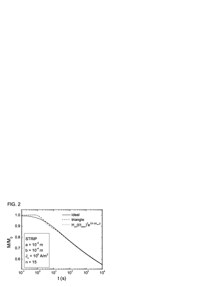
Figure 2: Magnetic relaxation curves computed for different magnetic field ramps in a thick strip.

We have initially computed the magnetic relaxations for a strip in perpendicular magnetic field (perpendicular geometry) by simulating a case analogous to the one discussed in the work of Jirsa et al Jirsa et al. (1993). In our computation $J_{c}=10^{9}$ A/m² and the critical exponent is $n=15$. We are considering a superconductor with large critical current density but with large creep. The external field ramps with a sweep rate of 1 mT/s up to 0.2 T, which is a value well above the full penetration field of the strip. Indeed, looking at the field profile we have verified that the strip is fully penetrated for fields higher than 0.10 T. As shown in Fig. 2, also if the overshoot does not occur in the field ramp, the magnetization decays non-logarithmically, especially at short time ($\leq$ 10 s). This result is expected due to the power law in the $E-J$ relationship which involves a logarithmic dependence of the pinning energy on the current density. In the same figure, a magnetic relaxation curve is shown as computed for a field ramp which has a triangular overshoot. In this case, the external magnetic field ramps up to 0.2 T. After this, the field overshoot occurs with an amplitude of $H_{ov}=1$ mT. The field overshoot reaches its maximum one second after the external field should have been stopped at the nominal target value. The external field goes down to the nominal value of 0.2 T after 5 seconds. Also in this case, when the magnetic field is stopped at the fixed value of 0.2 T the time derivative of $H_{a}$ is instantaneously zero. A more realistic situation have been considered by computing the magnetic relaxation for the case c) where $H_{ov}=1$ mT, $t_{ovm}=1$ s and $c=2$. The case c) is effectively realized in experiments, where the field cannot be stopped instantaneously and the overshoot shape is rounded.
As shown in Fig. 2, the magnetization curves in the cases b) and c)have an initial values $M_{i}$ larger than in the ideal case. In fact, when the overshoot occurs, the magnetization does not relax during the first seconds, since the magnetic field continues to increase. The largest value of the initial magnetization is obtained in the case of an exponential overshoot; indeed, the electrical field induced in the superconductor in the first seconds is larger than in the other cases (see also Fig. 1). When the external magnetic field rate reverses, the magnetization quickly decreases, because of the flux coming out from the surface, and after 5 seconds $M$ has lost the 12% of the initial value. The decay during the first 5 seconds depends on the shape of the field overshoot as function of the time. In the triangular case, the magnetization curve shows a convex concavity, whereas in the case c) the curvature is concave. After 5 seconds, the external field is practically constant and the magnetic relaxation effectively starts; for $t$ larger than 100 seconds the three curves join together. These computations confirm also in perpendicular geometry, the results found for parallel geometry in Ref.Jirsa et al., 1993. However in this case the field overshoot amplitude is 1% of the full penetration field. In the next section we will consider situations where the induced ESF state strongly affects the magnetic relaxation.

III.1 ESF state in slab

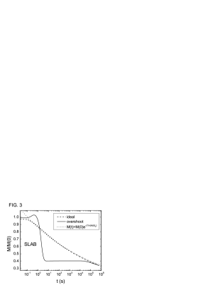
Figure 3: Magnetic relaxation curves computed for different magnetic field ramps in a slab. The dotted line is the relaxation given by the analytical formula reported in the text.

Figure 4: Time evolution of the magnetic field profiles in a slab; the initial field profile is achieved without field overshoot.

Figure 5: Time evolution of the magnetic field profiles in a slab, when a field overshoot occurs. The dotted lines represent the flux profiles which fully resemble the ideal profiles. The dashed lines represent the profile during field ramp rate reversing. Continuous lines show the field profiles in the time windows where the magnetization is nearly constant. In the inset a detail of the profile close to the slab surface is shown.

Here, we discuss the magnetic relaxation starting from an ESF state in the case of a slab in parallel field. In Fig. 3, two computed $M(t)$ curves are shown; the initial magnetic state is obtained by ramping the external field both in the ideal way (without overshoot) and with an overshoot of 1 mT (dashed curve) In the same figure, it is shown the magnetic relaxation (dotted line) for a superconducting slab, according to the relation given in Ref. Yeshurun et al., 1996, where it is assumed that the pinning energy depends logarithmically on the current density:

$$M(t)=M(0)\exp\left(-\frac{1}{n}\ln\left(\frac{t}{t_{0}}\right)\right)$$ (22)

The dimension of the slab used for the computations is $2a=10^{-4}$m, the critical current density $J_{c}=10^{8}$ A/m² and the exponent $n=15$. In this case the full penetration field of the slab is $H_{p}=6.3$ mT and thus it is of the same order of magnitude with respect to the overshoot (1 mT). As shown in Fig. 3, the computed ideal curve is approximated quite well by the analytical relation in the time range from 10 to 10⁴ seconds, whereas it wanders off each other at very short and very long times. On the other hand, we observe as the overshoot has effects on long time up to $10^{5}$ s (dashed curve). In the first 5 seconds, the magnetization looses 60% of the initial value due to the inversion of the flux profile close to the slab surface. In the subsequent 10⁴ seconds the magnetization practically does not relax, and after this time the relaxation rate increases. After 10⁶ seconds the magnetization computed with an ideal ramp and the curve computed with a field overshoot take the same value.
At this point, it is necessary to investigate if the magnetization computed for time larger than $3.0\ 10^{5}$ s in both the cases, corresponds to the same magnetic state. In order to answer this question, we have computed the magnetic field profiles as a function of time. In Fig. 4 and in Fig. 5, the field profiles computed for both the cases are shown. In particular, in Fig. 4, the profiles of the relaxation in a slab are shown, reproducing the usual Bean results. On the other hand, the profiles computed in the case of a relaxation from an ESF state, obtained by using the exponential overshoot, (Fig. 5 show that during the first 5 seconds the profile changes (dashed line) as a consequence of the field decreasing. The evolution of the profiles during the first 5 seconds has some difference in comparison with the classic Bean profile, where $J_{c}$ is constant and independent on the applied electrical field. In our case, while the flux is expelled on the surface, in the inner part of the slab the profile relaxes. This occurs because of the finite exponent $n$ which leads to a large creep. On the contrary, for the Bean model, the field profile, in the inner part of the slab, remains frozen during the field decreasing.
Starting from the fifth second the field profile relaxes overall in the slab and after $10^{5}$ seconds the magnetic profile becomes the ideal one. In Fig. 5 the field profiles which resemble the ideal ones are shown by dotted line. By means of our numerical simulations we have shown that the same magnetization value found in the two $M(t)$ curves corresponds to the same magnetic state. In Fig. 5, we observe also that the maximum of the field profile, due to the field ramp rate reversing, moves towards the slab edges during the relaxation. At the same time, the entrapped magnetization is reduced down to zero. Therefore the ESF state has relaxed towards a fully shielded state.
Increasing the amplitude of the overshoot, we expect that the ideal relaxation and the relaxation from a ESF state will coincide at longer times. Nevertheless, as the region with entrapped flux prevails on the shielded region, the flux profile relaxes towards a fully entrapped state.

III.2 ESF state in strip

Figure 6: Evolution field on time for a thick strip. The field profiles computed in the ideal case are shown on the upper frame. The field profiles computed when an overshoot occurs in the field ramp are shown on the lower frame.

Figure 7: zoom of the previous figures, in the region close to the strip edge.

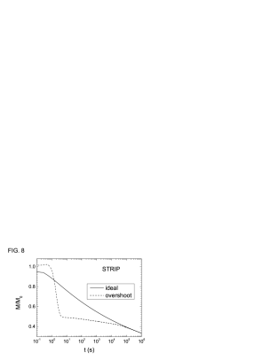
Figure 8: Magnetic relaxation curves computed from different magnetic field ramps in a thick strip.

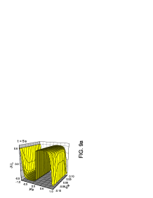
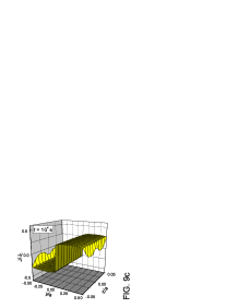
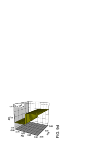
Figure 9: Current density distribution at different times for a strip. The current density is computed in the case of an overshoot in the field ramp.

In order to analyze the effect of the sample geometry on the relaxation, we considered the case of a strip in perpendicular field for which the main effect of the overshoot arises on the surface, where the demagnetizing field is more intense. In Fig. 6 the magnetic field profiles for a thick strip ($2a=$1 mm, $2b=$0.1 mm) are reported; a critical current density of $10^{8}$ A/m² and an $E-J$ exponent $n=15$ are set. In the upper part of the figure we can see the field profile relaxations in the ideal case. We can observe that the demagnetizing field relaxes towards lower magnetic fields on the surface. At the same time, the field increases in the inner region and there is a boundary, known as the neutral line, where the field remains constant; it divides the region with entrapped flux from the one with shielded flux. If an overshoot of a 1 mT occurs the flux, as expected, is strongly reduced on the strip edge and the field maximum is located inside the strip. In the next 10⁶ seconds the maximum relaxes and moves towards the strip edge where, at the same time, the field increases. On the contrary, in the ideal case the field on the border always decreases during the relaxation. When the maximum reaches the edge, the field profile in the strip fully resembles the profile computed in the ideal case and the relaxation continues as in the ideal case. Also in this case, as shown in the magnetization curves in Fig. 8, the $M(t)$ with and without overshoot join together at long times. Also in the perpendicular geometry the evolution of the magnetic state is directed to rebuild a shielded state. In Fig. 9, the time evolution of the current density is shown . During the relaxation the current changes sign and after long time the current distribution in the cross section of the strip rebuilds the distribution of a full shielded state. Except for the time evolution of the magnetic field on the border of the strip, in the perpendicular geometry there are not substantial differences respect to the parallel geometry. In fact, our computations have shown that in the perpendicular geometry, for $H_{a}>H_{p}$, the demagnetizing effects do not affect the time evolution of the magnetic relaxation.

IV Experimental Results and Discussion

Figure 10: Magnetic field ramp with a sweep rate of 3.3 mT/s in the time window where a field overshoot occurs, as measured by a hall-probe (square and line), and $H_{a}(t)$ employed in our computation (dotted line).

Magnetic relaxation measurements have been performed by means of a Vibrating Sample Magnetometer (VSM) equipped with a 16 T magnet. The external magnetic field can be ramped with a maximum sweep rate of 7 mT/s. When the field is nominally stopped the magnetic field has an overshoot of around 1$\div$5 mT depending on the sweep rate used for ramping the field and this unwanted feature has been used to induce a ESF state in our samples. We used a hall probe to measure the time dependence of the external field and in the inset of the Fig. 10 the measured overshoot for our magnet is shown.
In order to check of validity of our numerical results, we have measured the magnetic relaxation on monofilamentary BSCCO(2223)/Ag tapes prepared by the standard PIT technique. We have chosen this kind of samples because they allow us to study bulk rectangular samples with full penetration fields which can be in the order of 10 mT even at the lowest temperature i.e. 4.2 K. The dimensions of the superconducting region in the measured sample are 3.02 $\times$ 0.14 $\times$ 4.6 mm³ and the estimated critical current density ranges from $10^{7}$ to $10^{9}$ A/m², depending on the temperature. In this way we can study experimentally the overshoot effects as $H_{p}$ decreases.
$M(t)$ measurements have been performed with the field perpendicular to the sample surface ($H\parallel c$-axis) in the 4.2 - 45 K temperature range, cooling the sample in zero-field (ZFC) for each temperature. The initial magnetic state is obtained by increasing $H_{a}$ with a sweep rate of 3.3 mT/s, up to 2 T. After this, the field is decreased with the same sweep rate down to a measuring field $\mu_{0}H_{0}=1$ T. The field variation of 1 T is chosen to be, for any measuring temperature, well above $H_{p}$, which is evaluated by taking the value of the field corresponding to the maximum (in absolute value) in the virgin magnetization curves at 4.2 K. In this way, in absence of a field overshoot, a full critical state, with entrapped flux, is realized in the superconductors Yeshurun et al. (1996). As the final field $H_{0}$ is nominally achieved, the $M(t)$ data are acquired each second for 5000 seconds.

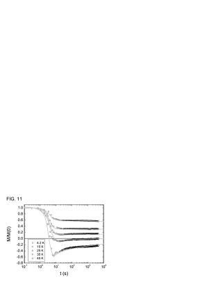
Figure 11: Magnetic relaxations measured at different temperatures for a magnetic field $H_{0}=$ 1 T (points) and computed curves (continuous lines).

Table 1: critical current densities and exponent $n$ used for the fit of the experimental curves.

$T$ (K)	$J_{c}$ (A/m2)	$\ n$
4.2	$2.40\ 10^{8}$	20
15	$1.15\ 10^{8}$	19
25	$9.70\ 10^{7}$	13
35	$8.70\ 10^{7}$	9
45	$4.00\ 10^{7}$	8

The $M(t)$, normalized at the initial magnetization value $M(0)$, measured at different temperatures, are shown in Fig. 11. In all the curves, a large drop in the magnetization occurs during the first 11 seconds and this time corresponds to time interval during which the external field has an overshoot. The behaviour of the magnetization in the subsequent 5000 seconds depends on the value of the temperature. At 4.2 K the magnetization decreases slightly, but the relaxation after 5000 seconds does not exhibit the behaviour expected for a fully entrapped state. At 15 K and 25 K, the magnetization remains nearly constant, whereas at 35 K and 45 K the magnetization first takes negative values and then increases on time. The effect of the overshoot increases as the full penetration field decreases with the temperature. These measurements show that the magnetic relaxation can be still affected by the field overshoot after at list 100 s. The negative values measured in the $M(t)$ at 45 K mean that the shielded flux region in the sample is larger than the entrapped one, although the initial condition was a fully entrapped state.

Figure 12: Field profiles computed for the relaxation at 45 K. The profile in the direction of the arrow are computed at $t=$100, 1000, 5000 s.

In order to reproduce our experimental results, we have computed the magnetic relaxation for a superconducting strip with the cross section of our sample. In the computations, the field ramp reproduces the experimental field ramp, with a sweep rate of 0.0033 T/s. The overshoot has been simulated by using the exponential function discussed in the Section III. As shown in Fig. 10, this function reproduces quite well the experimental overshoot with $H_{ov}=0.029$ mT, $t_{ovm}=1.7$ s and $c=1.3$. In our computation we have to set both $n$ and $J_{c}$. The exponent $n$ has been evaluated by measuring the hysteresis loop at different sweep rate. Taking the $M$ values measured at 1 T for different sweep rate ($\dot{B_{a}}$), $n$ is given by means of a linear fit of $\log(\dot{B_{a}})$ as function of $\log(M)$; the $n$ values reported in Tab. 1 have been rounded to the nearest integer. On the other hand, the critical current density is a free parameter chosen in order to obtain the best fit. From our computations, it results $J_{c}=2.4\ 10^{8}$ A/m² at 4.2 K and $4.0\ 10^{7}$ A/m² at 45 K. As shown in Fig. 11, the numerical computations reproduce well the experimental behaviour. In Fig. 12, the profile computed at T=45 K are shown. In particular, at t=10 s, when $H_{a}$ is practically constant, it results that the magnetic state in the superconductor has both the regions with entrapped and shielded flux. In the next 5000 seconds, the profile relaxes toward a shielded state, which is practically fulfilled at t=5000 s, when the simulation is stopped.
Our work shows that the first seconds of the relaxation have to be analyzed very carefully in order to estimate correctly the creep rate and, thus, extract information about the pinning properties of the sample. In fact, our results show that it is not appropriate just to cut the first seconds of the relaxation curves and extract information from the remanent data if the presence of an overshoot in the magnet has not been previously considered.

V Conclusion

In this work, we have studied the magnetic relaxation from a state with shielded and entrapped flux, generated by a field overshoot after the nominal stop of the external field. The magnetic relaxations have been computed in parallel and perpendicular geometry. The computed magnetization shows a large drop in the first seconds due to the flux expulsion from the samples boundary. After long time, the $M(t)$ curves computed with and without field overshoot (having, thus, as initial condition an ESF and a full shielded or entrapped flux state, respectively) join together. Moreover, our simulations show that, during the relaxation, the same value of the magnetization corresponds to the same magnetic state. In addition, the experimental relaxation curves, measured on BSCCO(2223) tapes, are well reproduced by our numerical computations, allowing us to correctly analyze the $M(t)$ from the instant when the external field is nominally stopped.