Nonlinear ac conductivity of interacting 1d electron systems

Abstract

We consider low energy charge transport in one-dimensional (1d) electron systems with short range interactions under the influence of a random potential. Combining RG and instanton methods, we calculate the nonlinear ac conductivity and discuss the crossover between the nonanalytic field dependence of the electric current at zero frequency and the linear ac conductivity at small electric fields and finite frequency.

I Introduction

In 1d electron systems, the effect of both interactions and random potentials is very pronounced, and a variety of unusual phenomena can be observed Giamarchi ; Gruner . The linear dc conductivity shows a power law dependence on temperature $T$ at higher temperatures Giamarchi+Schulz ; KaneFisher , but is exponentially small at low temperatures and vanishes at zero temperature Mott ; Shklovskii-Efros . The ac conductivity vanishes like MoHa68 $\sim\omega^{2}(\ln(1/\omega))^{2}$ and shows several cross-overs to other power laws at higher frequencies Fogler02 .

Much less is known about the non-linear conductivity. At zero temperature and frequency charge transport is only possible by tunneling of charge carriers, which can be described by instanton formation. The nonlinear dc-conductivity is characterized by S73 ; NaGiDo03 ; MaNaRo04 ; FoKe05 $I\sim\exp(-\sqrt{E_{0}/E})$ provided the system is coupled to a dissipative bath. Without such a coupling, the current was recently suggested to vanish below a critical temperature GoMiPo05 ; BaAlAl05 .

In this work, we calculate the low energy non- linear ac conductivity for systems with random pinning potentials and discuss the crossover between linear ac response at small fields and nonlinear dc response at large fields. To be specific, we consider a charge density wave (CDW) or spinless Luttinger liquid (LL) pinned by a random lattice potential which can be described by the quantum sine-Gordon model with random phases. We first scale the system to its correlation length, where the influence of the potential is strong and a semiclassical instanton calculation becomes possible. The response is dominated by energetically low lying two level systems (TLS), whose dynamics is described by a Bloch equation.

Microfabrication of quantum wires or 1d CDW systems slot+04 should allow to test our predictions experimentally. Indeed there is a number of recent experiments on carbon nanotubes TaSuWa00 ; CuZe04 ; TzChYi04 and polydiacetylen AlLeCh04 which seem to confirm the variable range hopping prediction for the dc-conductivity made in NaGiDo03 ; MaNaRo04 .

II AC conductivity of 1d disordered systems

In the following, we present a heuristic derivation Mott of the Mott–Halperin result MoHa68 for the ac conductivity of a one-dimensional disordered electron system without interactions. In the end of the section, we indicate how this result can be generalized to interacting electrons.

In one spatial dimension, all electron states are localized and wave function envelopes decay on the scale of the localization length $\xi_{\rm loc}$. We divide the system into segments with size $\xi_{loc}$. The typical energy separation of states within one segment is the mean level spacing $\Delta=1/(\rho_{F}\xi_{\rm loc})$, where $\rho_{F}$ is the density of states at the Fermi level per unit length. Levels in neighboring segments are coupled by the Thouless energy $t(\xi_{loc})=\Delta$. When we consider the coupling between more distant segments of separation $L$ the coupling is reduced to $t(L)=\Delta\exp(-L/\xi_{loc})$. The coupling splits (almost) degenerate energy levels in different segments by an amount $\Delta E=2t(L)$. Due to the coupling, the eigenstates of the Hamiltonian are even and odd linear combinations of states localized in segments a distance $L$ apart. A spatially constant ac electric field $E(t)=E_{0}\cos\omega t$ causes transitions between levels with a separation $\Delta E=\hbar\omega$, hence we demand $2t(L)=\hbar\omega$ and therefore

$$L_{x}(\omega)=\xi_{loc}\ln(2\Delta/\hbar\;\omega)\ .$$ (2.1)

According to Fermi’s golden rule, the transition rate for exciting the even linear combination to the odd one is given by $1/\tau={2\pi\over\hbar}\ {1\over 4}e_{0}^{2}E_{0}^{2}|\hat{x}_{\epsilon,\epsilon+\hbar\omega}|^{2}\ \rho_{F}\ \xi_{loc}$. Here, the matrix element $\hat{x}_{\epsilon,\epsilon+\hbar\omega}$ of the position operator has to be calculated between the ground state with energy $\epsilon$ and the excited state with energy $\epsilon+\hbar\omega$, it is found to be equal to the spatial separation $L_{x}(\omega)$ of the two localized states. When calculating the rate of energy absorption ${1\over 2}\sigma_{\rm ac}(\omega)E_{0}^{2}$ due to the excitations of such two level systems, one has to take into account that each photon carries the energy $\hbar\omega$, that only transitions from unoccupied states to occupied states are possible, and that the occupation probability for a state with energy $\epsilon$ is determined by the Fermi function $f(\epsilon)$. In this way, one finds

$$\sigma_{\rm ac}(\omega) = \int d\epsilon\rho_{F}\hbar\omega f(\epsilon)[1-f(\epsilon)]{2\pi\over\hbar}{e_{0}^{2}\over 2}L_{x}(\omega)^{2}\xi_{loc}\rho_{F}$$ (2.2)

$$\approx \sigma_{0}\ L_{x}^{2}(\omega)\ (\hbar\omega\rho_{F})^{2},\,\,\,\ \sigma_{0}=\frac{e^{2}_{0}}{\hbar}\xi_{loc}.$$

This result can be generalized to an interacting electron system FeVi81 by remembering the basic idea of bosonization: the charge density is defined as the derivative of a displacement field, and a localized electronic state corresponds to a localized kink in the displacement field. In addition, the density of states $\rho_{F}$ at the Fermi level has to be replaced by the compressibility $\kappa={\partial\rho\over\partial\mu}$. With these modifications, the above derivation can be repeated and one obtains an result analogous to Eq. (2.2).

It is worthwhile to remark that the ac-conductivity (2.2) can be rewritten as

$$\sigma_{\rm ac}(\omega)\sim\sigma_{0}\ e^{-2L_{x}(\omega)/\xi_{loc}}\ \left(\frac{L_{x}(\omega)}{\xi}\right)^{2},\,\,\,\$$ (2.3)

where $\xi$ is the correlation length of the system. This result resembles the form of the result for the non-linear dc-conductivity

$$\sigma_{\rm dc}(E)\sim\sigma_{0}\ \frac{\hbar\omega_{\rm e-ph}}{\Delta}\ e^{-2L_{x}(E)/\xi_{\rm loc}}\ \left(\frac{L_{x}(E)}{\xi}\right)^{2}\,\,\,\ \ .$$ (2.4)

Here $L_{x}(E)=\xi_{\rm loc}\sqrt{\frac{\Delta}{e_{0}E_{0}\xi_{\rm loc}}}$ denotes the spatial distance of the energy levels between which the tunneling events take place, it follows from a variational treatment S73 ; NaGiDo03 . The prefactor $\hbar\omega_{\rm e-ph}/e_{0}E_{0}\xi_{\rm loc}$ takes into account that the dissipation rate is controlled by the typical frequency for electron phonon coupling $\omega_{\rm e-ph}$ and that the current is hence of the order FoKe05 $\sim e_{0}\omega_{\rm e-ph}e^{-2L_{x}(E)/\xi_{\rm loc}}\,\,\,\,\,$. We note that depending on the details of the electron phonon coupling, $\omega_{\rm e-ph}$ may depend on the external electric field.

Finally, at finite temperatures, Mott variable range hopping gives a linear dc-conductivity which follows from (2.4) by replacing $L_{x}(E)$ by $L_{x}(T)=\sqrt{\Delta/k_{B}T}$, i.e.Mott ; Teber

$$\sigma_{\rm dc}(T)\sim\sigma_{0}\ \frac{\hbar\omega_{\rm ph}}{\Delta}\ e^{-2L_{x}(T)/\xi_{\rm loc}}\ \left(\frac{L_{x}(T)}{\xi}\right)^{2}\,\,\,\ \ .$$ (2.5)

The cross-over between the three expressions (2.3)-(2.5) can most easily be understood by the dominance of a shortest tunneling distance, as will be discussed further below.

III The Model

The models we analyze are defined by the euclidean action

$${S\over\hbar} = {1\over 2\pi K}\int dx\int_{0}^{v\hbar\beta}dy\left[\left({\partial\varphi\over\partial x}\right)^{2}+\left({\partial\varphi\over\partial y}\right)^{2}\right.$$

$$\left.-2u\cos(p\varphi+2\pi\zeta(x))+{2Ke_{0}\over\pi v}\varphi E(y)\right]\ +{S_{\rm diss}\over\hbar},$$

where we have rescaled time according to $v\tau\to y$, and $\beta=1/k_{B}T$. The dissipative part of the action describes a weak coupling of the electron system to a dissipative bath, for example phonons. It is needed for energy relaxation in variable range hopping processes MaNaRo04 and for equilibration in the presence of a strong ac field. We assume it to be so small that it does not influence the RG equations for the other model parameters significantly. The smooth part of the density is given by ${1\over\pi}\partial_{x}\varphi$, and $p=1,2$ for CDWs and LLs, respectively. We consider a CDW or LL with Gaussian disorder, which is described by $\zeta(x)$ equally distributed in the interval $[0,1]$ with correlation length equal to the lattice spacing $a$.

For $K>K_{c}(u)$ the potential is RG irrelevant and decays under the RG flow, while for $K<K_{c}(u)$ the potential is relevant and grows, here Giamarchi+Schulz $K_{c}(0)=6/p^{2}$ . We assume $K<K_{c}(u)$ and scale the system to a length $\xi=ae^{l^{\ast}}$, on which the potential is strong. After the scaling process, the parameters $K$, $v$, and $u$ in Eq. (III) are replaced by the effective, i.e. renormalized but not rescaled, parameters $K_{\rm eff}$, $v_{\rm eff}$, and $u_{\rm eff}$.

We note that the ratio $K/v$ and hence the compressibility $\kappa={K\over v\hbar\pi}$ is not renormalized due to a statistical tilt symmetry Schultz+88 . The compressibility $\kappa={\partial\rho\over\partial\mu}$ is used as a generalized density of states for interacting systems. Our calculations are valid for energies below the generalized mean level spacing $\Delta_{0}={1\over\kappa\xi}$.

In this RG calculation, we do not attempt to treat a possible nonlinear dependence of coupling parameters on the external electric field. The full inclusion of the external field in an equilibrium theory is not possible as it renders the ground state of the system unstable. The quantum sine-Gordon model has an infinite number of ground states connected by a shift of the phase field by $2\pi/p$. Here, we concentrate on renormalizing each of these ground states separately and take into account the coupling between different ground states due to the external electric field in the framework of an instanton approach.

IV Disordered LL or CDW

The wall width $1/\sqrt{p^{2}u_{\rm eff}}\approx\xi$ of an instanton solution to the action Eq. (III) is for weak external fields much smaller than the extension of the instanton. Hence, the instanton action can be expressed in terms of the domain wall position $X(y)$. The discussion of instantons in the case of random pinning is more involved than e.g. for periodic pinning Maki77 and the calculation of closed form instanton solutions is not possible. For this reason, we look for approximate instanton solutions with a rectangular shape and extensions $L_{x}$, $L_{y}$ in $x$– and $y$–direction, respectively. As the disorder is correlated in time but not in space, instanton walls in $x$– and $y$–direction contribute $L_{x}s_{y}$ and $L_{y}s_{x}(x)$ to the action, respectively. While the surface tension $s_{y}={2\pi\over p^{2}\xi K_{\rm eff}}$ is essentially constant, the surface tension $s_{x}$ has a strong and random position dependence. To calculate the statistical properties of $s_{x}$, we make use of the exact solution Glatz01 of the classical ground state of a LL or CDW with random pinning in the following.

In the limit $K_{\rm eff}\ll 1$, quantum fluctuations are strongly suppressed and the (classical) ground state of the model Eq. (III) can be determined exactly NaGiDo03 . After renormalization to the scale $\xi$, the effective action can be rewritten as a discrete model on a lattice with grid size $\xi$, and the integration over $x$ can be replaced by a summation over discrete lattice sites $i=x/\xi$. In the classical ground state, the solution $\varphi(x,y)$ does not depend on $y$ any more and the $y$–integral in Eq. (III) simply yields an overall factor $v_{\rm eff}\hbar\beta$. Dividing the action by $\hbar\beta$, one obtains the classical Hamiltonian NaGiDo03

$$H_{\rm class}={\Delta_{0}\over 2\pi^{2}}\sum_{i=1}^{L_{0}/\xi}[(\phi_{i+1}\!-\!\phi_{i})^{2}-2\xi^{2}u_{\rm eff}\cos(p\phi_{i}\!-\!2\pi\zeta_{i})]\;.$$ (4.1)

Here, $u_{\rm eff}$ is the disorder strength with $u_{\rm eff}\;\xi^{2}\gg 1$ and $\zeta_{i}\in[0,1]$ is a random phase. In the effective Hamiltonian Eq. (4.1), the disorder term dominates the kinetic term and the classical ground state of the system can be explicitly constructed Glatz01 . One minimizes the cosine potential for each lattice site by letting $p\phi_{i}=2\pi(\zeta_{i}+n^{0}_{i})$ with integer $n^{0}_{i}$. The set of integers $\{n^{0}_{i}\}$ is chosen in such a way that the elastic term in Eq. (4.1) is minimized,

$$n^{0}_{i}=m+\sum_{i<j}\left[\zeta_{i+1}-\zeta_{i}\right]_{G}\ \ .$$ (4.2)

Here, $[\zeta]_{G}$ denotes the closest integer to $\zeta$, and $m$ is an integer parameterizing the infinitely many equivalent ground states. Excitations of the ground state change $n_{i}^{0}\rightarrow n_{i}^{0}\pm 1$ for sites with $i_{0}<i<i_{0}+L_{x}/\xi$, they bifurcate from one ground state characterized by $m=m_{0}$ to another ground state with $m=m_{0}\pm 1$. The potential energy necessary for a bifurcation at position $i$ is according to Eq. (4.1)

$$\Delta H(i)\! = \!{\Delta_{0}\over 2\pi^{2}}(2\pi/p)^{2}\left\{1\pm 2\left((\zeta_{i}-\zeta_{i-1})-\left[\zeta_{i}-\zeta_{i-1}\right]_{G}\right)\right\}$$ (4.3)

$$\equiv \hbar v_{\rm eff}s_{y}g_{i}$$

with a random $g_{i}\in[0,2]$. Defining the localization length $\xi_{\rm loc}={p^{2}K_{\rm eff}\xi\over 2\pi}$, one has $s_{y}={1\over\xi_{\rm loc}}$.

Quantum effects are due to the time derivative in the action Eq. (III) and give rise to tunneling between the ground state and excited states in the presence of an external electric field. Similar to the case of periodic pinning Maki77 , these tunneling events are described by instantons. In the following, we describe how the action of a quadratic instanton can be calculated.

The action of a bifurcation with extension $L_{y}$ is just $\Delta H(i_{0})L_{y}/v_{\rm eff}$. The action of a wall with constant $y$ and length $L_{x}$ can be calculated by an analogous consideration if one introduces a lattice of grid size $\xi$ in $y$–direction. As the disorder is correlated in time direction, one needs not consider random phases $\zeta_{i}$ and finds an action $\hbar s_{y}L_{x}$. Adding up the contributions from all four walls of an instanton, one finds the action of a rectangular $L_{x}\times L_{y}$–instanton NaGiDo03

$${\Delta S\over\hbar}=\left(s_{x}(i_{0})+s_{x}(i_{0}+L_{x})\right)L_{y}+2s_{y}L_{x},\,\,\,\ s_{x}(i)=s_{y}g_{i}.$$ (4.4)

In a noninteracting electron system, a pair of sites with $g_{i}\ll 1$ corresponds to an electron with energy $-\epsilon_{1}=-g_{1}\Delta_{0}$ just below the Fermi level at position $i_{0}$, which can hop to an unoccupied level with energy $\epsilon_{2}=g_{2}\Delta_{0}$ just above the Fermi level at position $i_{0}+L_{x}$. The translation between the language of noninteracting elctrons and the bosonic language used in this calculation is summarized in Table 1.

Typically, the two lowest $g_{i}$ in an interval of length $L_{x}$ are of the order $1/L_{x}$, and the boundaries of a typical instantons will be at positions with a small surface tension $s_{x}\approx s_{y}\xi/L_{x}$. Taking into account the contribution of a dc external electric field, the total action of a typical instanton is

$${S(L_{x},L_{y})\over\hbar}=2s_{y}{\xi\over L_{x}}L_{y}+2s_{y}L_{x}-{2e_{0}E_{0}\over p\pi v_{\rm eff}\hbar}L_{x}L_{y}\ \ .$$ (4.5)

Extremizing the action with respect to $L_{x}$, $L_{y}$ one finds NaGiDo03

$$L_{x}(E)=\sqrt{2\pi\over p\kappa e_{0}E_{0}}\ ,\ \ \ L_{y}={\pi\over p\kappa\xi e_{0}E_{0}}\ \ .$$ (4.6)

The creation rate of these instantons is

$$P_{\rm random}\sim e^{-2L_{x}(E_{0})/\xi_{\rm loc}}\ \ ,$$ (4.7)

leading to the result Eq. (2.4) for the conductivity.

Table 1: Translation between boson and electron language.

electron language	boson language
particle	kink
hole	antikink
$\rho(x)$	${1\over\pi}\partial_{x}\varphi$
surface tension $s_{x}(i_{0})$	energy $-\epsilon_{1}(i_{0})$
surface tension $s_{x}(i_{0}+L_{x})$	energy $\epsilon_{2}(i_{0}+L_{x})$

Next we consider an ac field $E(t)$, which upon analytical continuation $it\to\tau$ turns into a field $E(\tau)$. In imaginary time, the electric field has to obey the same periodic boundary condition $E(\tau+\beta)=E(\tau)$ as other bosonic fields, e.g. the displacement field $\varphi(\tau)$. This boundary condition is respected by a discrete Fourier representation NeOr88

$$E(\tau)=T\sum_{\omega_{n}}E(\omega_{n})e^{-i\omega_{n}\tau},\ \ \ \omega_{n}={n2\pi k_{B}T\over\hbar}$$ (4.8)

with Matsubara frequencies $\omega_{n}$. A monochromatic external field is hence described by $E(y)=E_{0}\cos\tilde{\omega}_{n}y$, where time is rescaled as $y=v_{\rm eff}\tau$ and frequency as $\tilde{\omega}_{n}=\omega_{n}/v_{\rm eff}$. In the end of our calculation, we analytically continue Matsubara frequencies to retarded real frequencies $i\tilde{\omega}_{n}v_{\rm eff}\to\omega+i\eta$.

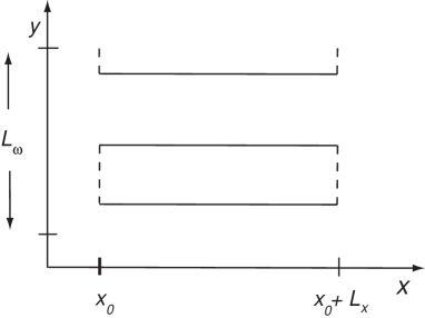
Figure 1: Hopping of kinks from position $x_{0}$ to $x_{0}+L_{x}$ or back (full lines) in a time interval of length $L_{y}$. The lines parallel to the $y$–axis do not contribute to the action if the line tensions $s_{x}$ are neglected.

Which type of instantons determines the current in the presence of an ac field with period $L_{\omega}=2\pi/\tilde{\omega}_{n}$? In the limit of a very small external electric field, the only external length scale in the problem is the ac period $L_{\omega}$, and the contribution of typical instantons to the linear response can be estimated by assuming that $L_{y}$ has to be of order $L_{\omega}$. A typical instanton obtained from minimizing Eq. (4.5) with respect to $L_{x}$ for a fixed $L_{y}=L_{\omega}$ and for vanishing $E_{0}$ has $L_{x}=\sqrt{\xi L_{\omega}}$. For this solution, the current would be proportional to $\exp[-{8\pi\over p^{2}}(1+i)\sqrt{\Delta_{0}/\hbar\omega}]$ and vanish nonanalytically for small frequencies. However, according to the Mott-Halperin law, the true frequency dependence should be proportional to MoHa68 $\omega^{2}\ln^{2}(1/\omega)$ . We conclude that typical instantons do not yield the leading contribution to the current and that a discussion of rare instantons is needed.

Indeed, besides typical instantons with $s_{x}\approx s_{y}\xi/L_{x}$, there are rare instantons with an exceptionally low $s_{x}(i)+s_{x}(i+L_{x})$. Such a pair of sites $i$ and $i+L_{x}$ allows for the hopping of a kink without changing the kink’s potential energy much. The potential energy difference $\epsilon_{1}+\epsilon_{2}$ between two sites can become arbitrarily small in sufficiently large samples. For the following considerations, we will set it to zero in the sense that it is much smaller than any other energy scale in the system. In the discussion of the dc electric field, quantum fluctuations, i.e. spontaneous creation of typical instantons in the absence of an external field, were unimportant. For pairs of sites with exceptionally low surface tensions, quantum fluctuations are important and have to be taken into account. Here, the spontaneous formation of instantons describes the physics of level repulsion NeOr88 . In our approximation of vanishing $s_{x}$, the instanton action does not depend on the extension $L_{y}$ in time direction any more, hence the occurrence of single domain walls of length $L_{x}$ with constant $y$ is possible. Such a domain wall describes the hopping of a kink across the distance $L_{x}$, and its action is

$$S_{single}/\hbar=s_{y}L_{x}\ .$$ (4.9)

To obtain the partition function for this tunneling degree of freedom, we must sum over all possible domain wall configurations in the interval $L_{\omega}$. A configuration with three hopping events is displayed in Fig. 1. Summation over all possible configurations yields

$$Z(L_{\omega}) = \sum_{n=0}^{\infty}{1\over n!}\prod_{i=1}^{n}\left(\int_{0}^{L_{\omega}}{dy_{i}\over\xi K_{\rm eff}}\right)e^{-ns_{y}L_{x}}$$

$$= \sum_{n=0}^{\infty}{1\over n!}\left({L_{\omega}\over\xi K_{\rm eff}}e^{-s_{y}L_{x}}\right)^{n}$$

$$= \exp\left({L_{\omega}\over\xi K_{\rm eff}}\ e^{-s_{y}L_{x}}\right)\ .$$

The integration measures in the $y_{i}$–integrals are normalized by $\xi K_{\rm eff}$ rather than by $\xi$ because the short time cutoff $\hbar/\Delta_{0}$ is determined by the high energy cutoff $\Delta_{0}$ and not by the short distance cutoff $\xi$. We note that the exponent of the outer exponential function is positive, indicating a lowering of the ground state energy due to frequent tunneling between the degenerate states. The summation over all possible instanton configurations describes the quantum mechanical effect of level repulsion. Coupled energy levels repel each other and are separated at least by

$$t_{0}(L_{x})=-\frac{\hbar v_{eff}}{L_{\omega}}\ln Z(L_{\omega})=\Delta_{0}\exp(-L_{x}/\xi_{\rm loc})\ .$$ (4.11)

The probability to have exactly one instanton (hopping of a kink forth and back) within the time interval $L_{\omega}$ is given by

$$p_{1}(L_{x}) = e^{-2s_{y}L_{x}}/Z(L_{\omega})$$

$$= \exp\left(-{L_{\omega}\over\xi K_{\rm eff}}e^{-s_{y}L_{x}}-2s_{y}L_{x}\right)\ .$$

The optimal length $L_{x}$ for such an instanton is found by minimizing the exponent in Eq. (IV) with respect to the tunneling length. We find

$$L_{x}={1\over s_{y}}\ln{L_{\omega}\over 2\xi K_{\rm eff}}\ .$$ (4.13)

Using this expression for $L_{x}$, we find the probability for having exactly one instanton of length $L_{\omega}$

$$p_{1}=e^{-2}\;\left({2\xi K_{\rm eff}\over L_{\omega}}\right)^{2}=\left({\tilde{\omega}_{n}\xi K_{\rm eff}\over e\;\pi}\right)^{2}\ \ .$$ (4.14)

This proportionality of the tunneling probability to frequency squared is the essence of the Mott–Halperin conductivity Eq. (2.2).

With the knowledge of the probability Eq. (4.14) for an instanton in resonance with the external field, we can now set up a calculation of the ac current. It is calculated as a derivative $I(x,\omega_{n})=-\hbar{\delta\over\delta a(x,-\omega_{n})}\ln Z$ of the partition function with respect to the vector potential $a(x,\omega_{n})=E(x,\omega_{n})/\omega_{n}$. The field $\phi$ couples to the vector potential via

$$S_{E}/\hbar={e_{0}\over\pi\hbar}\int dx\;{1\over\beta v_{\rm eff}}\;\sum_{\tilde{\omega}_{n}}a(x,-\tilde{\omega}_{n})(-\tilde{\omega}_{n})\phi(x,\tilde{\omega}_{n})\ ,$$ (4.15)

where $\beta$ denotes the inverse temperature. Hence, the current is given by

$$I(x,\tilde{\omega}_{n})=-e_{0}\;\tilde{\omega}_{n}v_{\rm eff}{\int D[\phi]\phi(\tilde{\omega}_{n})e^{-S[\phi]/\hbar}\over\int D[\phi]e^{-S[\phi]}}\ .$$ (4.16)

In the low energy regime, we do not perform the full functional integral over $\phi$ in order to evaluate the partition function. Instead, we sum over the relevant tunneling degrees of freedom. We label such a degree of freedom by the position $i_{0}$ of the first weak link and by the distance $L_{x}$ between the first and the second weak link. The field $\phi(i_{0})\;=\;\phi(i_{0}+1)\;=...=\phi(i_{0}+L_{x})$ takes the values $\phi_{0}$ and $\phi_{0}+2\pi/p$, respectively. Furthermore, we make use of the self averaging properties of the current. Instead of averaging it over the position $x$ in the system and let all different types of TLSs contribute to it, we calculate the contribution of one TLS and average over the parameters $L_{x}$, $s_{x}(i_{0})$, and $s_{x}(i_{0}+L_{x})$. So far we considered instantons with vanishing surface tension $s_{x}=0$. We now extend these considerations to instantons with surface energies smaller than $\hbar\omega$, i.e. we are concentrating on sites with $g_{i}<K_{\rm eff}\xi\tilde{\omega}_{n}$, where $s_{x}(i_{0})=s_{y}g_{1},\,s_{x}(i_{0}+L_{x})=s_{y}g_{2}$. The probability that the position $x$, for which we want to evaluate the current, is inside an active instanton is $L_{x}/\xi$ times the probability for finding a weak tunneling link at a given site. In this way, we obtain for the average current

$$\langle I\rangle(\tilde{\omega}_{n}) = -e_{0}\tilde{\omega_{n}}v_{\rm eff}\int{dg_{1}}{dg_{2}}{dL_{x}\over\xi}\ {L_{x}\over\xi}\ p_{1}(L_{x})\cdot$$ (4.17)

$$\cdot\int{dy_{1}\over\xi K_{\rm eff}}{dy_{2}\over\xi K_{\rm eff}}\ \phi_{0}(\tilde{\omega}_{n};y_{1},y_{2})\ e^{-S_{E}[\phi_{0}]}$$

Here, we evaluate the current under the approximation that there is exactly one instanton (two tunneling events at times $y_{1}$ and $y_{2}$) in the interval of length $L_{\omega}$. The two $g_{i}$ integrals contribute a factor $(K_{\rm eff}\xi\tilde{\omega}_{n})^{2}$ as we neglect the dependence of $S_{E}$ on the $g_{i}$. The integral over $L_{x}$ is evaluated by the saddle point method just taking into account instantons of the optimal length $L_{x}={1\over s_{y}}\ln{L_{\omega}\over 2\xi K_{\rm eff}}$. As $p_{1}$ is a function of $L_{x}/\xi_{\rm loc}$, we have to use the same variable in the integration measure to perform a saddle point approximation and obtain a factor $\xi_{\rm loc}/\xi$ from this transformation. If $y_{1}$ is the time of the first tunneling event and $y_{2}$ the time of the second tunneling event, we define the new variables $\tilde{y}=(y_{1}+y_{2})/2$ and $L_{y}=y_{2}-y_{1}$. The Fourier transform of the displacement field $\phi$ for such an instanton is given by

$$\phi(\tilde{\omega}_{n};L_{y},\tilde{y})={1\over\pi}\ e^{i\tilde{\omega_{n}}\tilde{y}}\ \sin{\tilde{\omega}_{n}L_{y}\over 2}\ .$$ (4.18)

For this field configuration, the coupling to the external electric field contributes the action

$$S_{E}(L_{y},\tilde{y})/\hbar = {e_{0}E_{0}L_{x}\over\pi\hbar v_{\rm eff}}{2\over\tilde{\omega}_{n}}\sin(\tilde{\omega}_{n}\tilde{y})\ \sin(\tilde{\omega}_{n}L_{y}/2)\ .$$

The barrier size is not fixed by the electric field as in the dc limit, and one has to consider both forward and backward jumps as for the standard thermally assisted flux flow argument AnKi64 . Hence, the probability for the instanton to be in phase with the external field is given by $2\sinh[S_{E}(L_{\omega},L_{x})/\hbar]$. Expanding to linear order in $S_{E}$ and integrating over $L_{y}$ and $\tilde{y}$, we find for the current

$$\langle I\rangle(\tilde{\omega}_{n}) = -e_{0}v_{\rm eff}\tilde{\omega}_{n}\ \ ({\tilde{\omega}_{n}\xi K_{\rm eff}\over e\;\pi})^{2}\ \ (\tilde{\omega}_{n}\xi K_{\rm eff})^{2}\ \ {L_{x}\over\xi}{\xi_{\rm loc}\over\xi}$$ (4.20)

$$\int_{0}^{L_{\omega}/2}\!\!\!\!{d\tilde{y}\over\xi K_{\rm eff}}\int_{0}^{L_{\omega}}\!\!\!\!{dL_{y}\over\xi K_{\rm eff}}\ \phi(\tilde{\omega}_{n};L_{y},\tilde{y})\ {2S_{E}(L_{y},\tilde{y})\over\hbar}$$

$$= -{8\over e^{2}}\;{e_{0}^{2}\over\hbar}\;\xi_{\rm loc}\;L_{x}^{2}\;\;\tilde{\omega}_{n}^{2}\;K_{\rm eff}^{2}\ E_{0}\ \ .$$

After the analytical continuation $\tilde{\omega}_{n}v_{\rm eff}\to-i\omega$ the real part of the conductivity agrees with formula Eq. (2.2) up to a numerical factor. As both $\xi_{\rm loc}$ and $L_{x}$ are proportional to $K_{\rm eff}$, the conductivity contains a factor of $K_{\rm eff}^{5}$ in agreement with the result FeVi81 ; Fogler02 .

V Description by Bloch equation

The instanton calculation presented in the last section needs to be improved upon in two respects: first, the classical level separation parameterized by the $g_{i}$ was not fully taken into account, and second, nonlinear correction in the strength of the external field are not considered yet. To achieve these goals, we use the concepts developed in the last section in a real time quantum mechanical calculation. Instantons in the imaginary time formalism correspond to the hopping of kinks from one level just below the chemical potential to another level just above the chemical potential. The localized states of a 1d disordered system can be modeled by an ensemble of these TLSs, and the average properties of the system can be calculated by averaging over the parameters of the TLSs.

We consider a TLS with spatial extension $L_{x}$ and on site energies $-\epsilon_{1}$ and $\epsilon_{2}$ with $\epsilon_{i}=g_{i}\Delta_{0}$. In a system of noninteracting electrons, the negative energy $-\epsilon_{1}$ corresponds to a particle below the Fermi level, and the positive energy $\epsilon_{2}$ to an unoccupied site above the Fermi level. The two sites are coupled by a distance dependent hopping integral $t_{0}(L_{x})$ according to Eq. (4.11). Such a TLS is described by the Hamiltonian $\hat{H}=\hat{H}_{0}+\hat{H}_{E}$ with

$$\hat{H}_{0}={1\over 2}(\epsilon_{1}+\epsilon_{2})\sigma_{z}-t_{0}(L_{x})\;\sigma_{x},\hat{H}_{E}={1\over 2}\ e_{0}L_{x}E_{0}\cos\omega t\ \sigma_{z}\ .$$ (5.1)

The position of the tunneling kink is measured by the operator $\hat{x}={1\over 2}L_{x}\sigma_{z}$, and the current operator is given by $\hat{I}=\rho(\epsilon_{1},\epsilon_{2},L_{x})e_{0}\dot{\hat{x}}$. Here,

$$\rho(\epsilon_{1},\epsilon_{2},L_{x})={1\over\xi}{d\epsilon_{1}\over\Delta_{0}}{d\epsilon_{2}\over\Delta_{0}}{dL_{x}\over\xi}$$ (5.2)

denotes the spatial density of TLSs with given parameter values. $\hat{H}_{0}$ is diagonalized by the unitary transformation

$$\hat{H}\to\exp(i\varphi\sigma_{y}/2)\hat{H}\exp(-i\varphi\sigma_{y}/2)$$ (5.3)

with $\varphi=\arctan{2t(L_{x})\over\epsilon_{1}+\epsilon_{2}}$. In the new basis, $\hat{H}_{0}$ corresponds to a static field in $z$–direction, and $\hat{H}_{E}$ to an oscillating field with $x$–component proportional to $\sin\varphi$ and $z$–component proportional to $\cos\varphi$.

In principle, the transformed Hamiltonian should now be solved in a nonequilibrium setup in a dissipative environment. In general, this type of problem is difficult to deal with in full generality Weiss99 . However, the problem simplifies if one does not treat an individual quantum system but averages over a whole ensemble instead. Such an ensemble of TLSs or spins interacting with an oscillatory electric field and subject to relaxation processes can be described by Bloch equations CoDiLa77 . We denote the ensemble polarization of the TLSs in the transformed basis by the pseudospin vector $\underline{p}$. The current $I$ is then proportional to the the pseudospin component in $y$–direction,

$$I=-{1\over 2}p_{y}\rho(\epsilon_{1},\epsilon_{2},L_{x})e_{0}L_{x}{t_{0}(L_{x})\over\hbar}\ .$$ (5.4)

The pseudospin polarization $\underline{p}$ of the TLSs follows the Bloch equation

$${d\over dt}\;{\underline{p}}=-{1\over\tau_{0}}\;(\underline{p}-\underline{p}_{0})+\alpha\;{\underline{p}}\times\underline{E}\ \ .$$ (5.5)

Here, $\underline{E}=\left[E_{0}\sin(\varphi)\cos(\omega t),0,{2\Delta\over eL_{x}}+E_{0}\cos(\varphi)\cos(\omega t)\right]$, $\underline{p}_{0}=[0,0,-1]$, $\Delta=\sqrt{(\epsilon_{1}^{2}+\epsilon_{2}^{2})/4+t_{0}^{2}(L_{x})}$, and $\alpha=e_{0}L_{x}/\hbar$. Inelastic processes are described by the phenomenological damping constant $\tau_{0}$. In the absence of an external electric field, the pseudospin relaxes due to this damping to its equilibrium value $\underline{p}_{0}$, i.e. the particle is in a superposition of states localized at $i_{0}$ and $i_{0}+L_{x}$. At temperatures much lower than the hopping integral $t_{0}(L_{x})$, the dissipative bath cannot destroy this coherent superposition and localize the particle, as the localized states have a higher energy than the symmetric linear combination.

The solution of Eq. (5.5) is described in detail in reference CoDiLa77 and we do not reproduce it here. We find that to order $O(E_{0}^{3})$, one type of TLS contributes to the conductivity

$$\sigma_{\rm TLS}(\omega;\!\epsilon_{1},\!\epsilon_{2},\!L_{x}\!) = \rho(\!\epsilon_{1},\!\epsilon_{2},\!L_{x}\!)\;{e_{0}^{2}L_{x}^{2}t^{2}(L_{x})\over 2\hbar^{2}\Delta}\cdot$$ (5.6)

$$\cdot{-i\over\omega-{2\Delta\over\hbar}-i{\hbar\over\tau_{0}}}\left[1-{1\over\hbar^{2}\Delta^{2}}\;{(e_{0}L_{x}E_{0}t_{0}(L_{x}))^{2}\over(\omega-{2\Delta\over\hbar})^{2}+{1\over\tau_{0}^{2}}}\right]\!.$$

The reduction of the linear conductivity becomes effective for strong ac fields, when both states of the TLS are occupied with comparable probability. In order to calculate the conductivity of the disordered sample, we integrate over all possible parameter values $\epsilon_{1}$, $\epsilon_{2}$, and $L_{x}$ and obtain the final result

$${\rm Re}\sigma_{\rm ac}(\omega)\!=\!\sigma_{0}{\pi\over 4}L^{2}_{x}(\omega)(\hbar\omega\kappa)^{2}(1\!-\!2\!{e_{0}^{2}L_{x}(\omega)^{2}E_{0}^{2}\over\hbar^{2}/\tau_{0}^{2}})$$ (5.7)

with the optimal tunneling length given by

$$L_{x}(\omega)=\xi_{\rm loc}\ln{2\Delta_{0}\over\hbar\omega}\ \ .$$ (5.8)

The linear part of Eq. (5.7) is proportional to $K_{\rm eff}^{5}$ and agrees with the result of Fogler Fogler02 . This linear conductivity describes the response of a disordered 1d system in region MH of Fig. 2. For an unscreened Coulomb interaction, in Eq. (5.7) one factor of $\hbar\omega$ has to be replaced by S81 $e_{0}^{2}/\epsilon L_{x}(\omega)$, where $\epsilon$ is the dielectric constant of the system.

When $e_{0}E_{0}L_{x}(\omega)\approx\hbar/\tau_{0}$, higher order terms become important and the ac current will saturate as a function of $E_{0}$. The value $E_{s}$ of the electric field where the current saturates can be estimated from Eq. (5.7) as

$$E_{s}={\hbar\over e_{0}\tau_{0}L_{x}(\omega)}\ \ .$$ (5.9)

As the nonlinear conductivity is defined as the ratio of current and electric field, in the saturation regime one obtains

$$\sigma_{\rm ac}(\omega,E>E_{s})=\sigma_{0}{p\over 8}L_{x}(E)^{2}{L_{x}(\omega)\over\xi}{\hbar\over\tau_{0}\Delta_{0}}(\hbar\omega\kappa)^{2}\ \ .$$ (5.10)

The region in $\omega$-$E$ space where the nonlinear conductivity Eq. (5.10) can be observed is labeled MHS in Fig. 2.

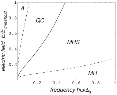
Figure 2: Different transport regimes in a disordered CDW or LL with dissipation as a function of field strength in units of $E_{\rm threshold}=\Delta_{0}/pe_{0}K_{\rm eff}\xi_{\rm loc}$ and frequency: adiabatic quantum creep in A, quantum creep with increased current noise in QC, ac conductivity following a Mott-Halperin law in MH, Mott-Halperin law with saturation for large field strengths in MHS.

VI Discussion

How does the linear conductivity Eq. (5.7) connect to the creep current in strong fields? The calculation of the nonlinear dc conductivity involves the optimal length scale $L_{x}(E)$ in Eq. (4.6) for tunneling processes. The crossover from ac to dc conductivity takes place when the two length scales $L_{x}(\omega)$ and $L_{x}(E)$ match, i.e. for a crossover frequency

$$\omega_{\times}={\Delta_{0}\over\hbar}e^{-L_{x}(E_{0})/\xi_{\rm loc}}\ .$$ (6.1)

For $\omega\approx\omega_{\times}$, the magnitude of the creep current $I_{\rm creep}\sim\exp(-2L_{x}(E)/\xi_{\rm loc})$ agrees with the magnitude of the ac current described by the conductivity Eq. (5.7), as the $\omega^{2}$ term in Eq. (5.7) matches the exponential dependence on field strength of $I_{\rm creep}$. Then, the expression Eq. (5.10) turns into

$$\sigma(E)=\sigma_{0}{p\over 8}{\hbar\over\tau_{0}\Delta_{0}}{L_{x}(E)^{3}\over\xi^{3}}e^{-2L_{x}(E)/\xi_{\rm loc}}\ \ ,$$ (6.2)

providing us with an estimate of the prefactor of the exponential factor describing dc creep. Identifying $\hbar/\tau_{0}\Delta_{0}$ as a dimensionless measure for the dissipation strength, this estimate agrees with a more sophisticated calculation, in which a TLS is coupled to phonons with an Ohmic spectral function Rosenow04 .

In the crossover region $\omega\approx\omega_{\times}$ between regimes QC and MHS in Fig. 2, there are two different types of TLS contributing to the current. In the ground state of a typical TLS with bare energy difference $\epsilon_{1}+\epsilon_{2}\approx\Delta_{0}\xi/L_{x}(E)\gg t(L_{x})$, most of the charge is localized at one of the levels. Under the influence of an external field, the charge hops irreversibly from one level to the other , as the hop is generally accompanied by an inelastic process. On the other hand, the ground state of a TLS with exceptionally low bare energy separation $\epsilon_{1}+\epsilon_{2}\leq t(L_{x})$ is the even parity combination of wave functions centered around the individual levels, and absorption of a photon excites the TLS to the odd parity state.

In the quantum creep regime, the time dependence of the current is calculated using the time dependent field in the formula for the dc current $I_{\rm creep}$. The adiabatic regime (region A in Fig. 2) is reached for frequencies smaller than the dc hopping rate $I_{\rm creep}/e_{0}$. While the average current is stronger than the current noise in the adiabatic regime, the current noise is stronger than the current for $I_{\rm creep}/e_{0}<\omega<\omega_{\times}$.

In summary, we have discussed the crossover from a nonlinear creep current in a static electric field to the linear ac response in 1d disordered interacting electron systems. While the linear ac conductivity is described by a generalized Mott-Halperin law, for stronger fields one finds a reduction of this linear conductivity as both states of a TLS are occupied with comparable probability. The crossover between nonlinear ac conductivity and dc creep current occurs when the spatial extension of TLSs matches the length scale for tunneling of kinks.

- (1) T. Giamarchi, Quantum Physics in One Dimension (Oxford Univ. Press, 2003).
- (2) G. Grüner, Density Waves in Solids (Addison-Wesley, New York, 1994).
- (3) T. Giamarchi and H. J. Schulz, Phys. Rev. B 37, 325 (1988).
- (4) C. L. Kane and M. P. A. Fisher, Phys. Rev. B 46, 15233 (1992).
- (5) N.F. Mott and E.A. Davis, Electronic Processes in Non-Crystalline Materials 2nd. ed., Clarendon Press, Oxford (1979).
- (6) B.I. Shklovskii and A.L. Efros, Electronic Properties of Doped Semiconductors, Springer (1984).
- (7) N.F. Mott, Philos. Mag. 17, 1259 (1968); B.I. Halperin, as cited by Mott.
- (8) M. Fogler, Phys. Rev. Lett. 88, 186402 (2002).
- (9) B. I. Shklovskii, Fiz. Tekh. Poluprovod. 6, 2335 (1972) [Sov. Phys.–Semicond. 6, 1964 (1973)].
- (10) T. Nattermann, T. Giamarchi, and P. Le Doussal, Phys. Rev. Lett. 91, 056603 (2003).
- (11) S. Malinin, T. Nattermann, and B. Rosenow, Phys. Rev. B 70, 235120 (2004).
- (12) M.M. Fogler and R.S. Kelley, cond-mat/0504047
- (13) I.V. Gornyi, A.D. Mirlin, and D.G. Polyakov, eprint cond-mat/0506411 (2005).
- (14) D.M. Basko, I.L. Aleiner, and B.L. Altshuler, eprint cond-mat/0506617 (2005).
- (15) E. Slot, H.S.J. van der Zant, K. O’Neill, and R.E. Thorne, Phys. Rev. B 69, 073105 (2004).
- (16) Z.K. Tang, D.D. Sun, and J. Wang, Physica B 279, 200 (2000).
- (17) J. Cummings and A. Zettl, Phys. Rev. Lett. 93 0868011 (2004).
- (18) M. Tzolov et al., Phys. Rev. Lett. 92, 0755051 (2004).
- (19) A.N. Aleshin et al., Phys. Rev. B 69, 214203 (2004).
- (20) M.M. Fogler, S. Teber, and B.I. Shklovskii, Phys. Rev. B 69, 035413 (2004).
- (21) U. Schultz, J. Villain, E. Brezin, and H. Orland, J. Stat. Phys. 51, 1 (1988).
- (22) K. Maki, Phys. Rev. Lett. 39, 46 (1977).
- (23) A. Glatz and T. Nattermann, Phys. Rev. B 69, 115118 (2004).
- (24) J.W. Negele and H. Orland,Quantum Many-Particle Systems, Addison-Wesley (1988).
- (25) P. W. Anderson and Y. B. Kim, Rev. Mod. Phys.36, 39 (1964).
- (26) M. V. Feigelman and V. M. Vinokur, Physics Letters A 87 (1-2): 53-60 (1981).
- (27) U. Weiss, Quantum Dissipative Systems, World Scientific (1999).
- (28) C. Cohen-Tannoudji, B. Diu, and F. Laloë, Quantum Mechanics Vol. II, John Wiley (1999).
- (29) B.I. Shklovskii and L. Efros, Zh. Eksp. Teor. Fiz. 81, 406 (1981) [ Sov. Phys. JETP 54, 218 (1981)].
- (30) B. Rosenow, to be published.