Transport Phenomena and Structuring in Shear Flow of Suspensions near Solid Walls

Abstract

In this paper we apply the lattice-Boltzmann method and an extension to particle suspensions as introduced by Ladd et al. to study transport phenomena and structuring effects of particles suspended in a fluid near sheared solid walls. We find that a particle free region arises near walls, which has a width depending on the shear rate and the particle concentration. The wall causes the formation of parallel particle layers at low concentrations, where the number of particles per layer decreases with increasing distance to the wall.

I Introduction

Many manufacturing processes involve the transport of solid particles suspended in a fluid in the form of slurries, colloids, polymers, or ceramics. Examples include the transport of solid material like grain or drug ingredients in water or other solvents through pipelines. Naturally, these systems occur in mud avalanches or the transport of soil in water streams. It is important for industrial applications to obtain a detailed knowledge of those systems in order to optimize production processes or to prevent accidents.

For industrial applications, systems with rigid boundaries, e.g. a pipe wall, are of particular interest since structuring effects might occur in the solid fraction of the suspension. Such effects are known from dry granular media resting on a plane surface or gliding down an inclined chute P. Mijatović (2002); T. Pöschel (1993). In addition, the wall causes a demixing of the solid and fluid components which might have an unwanted influence on the properties of the suspension. Near the wall one finds a thin lubrication layer which contains almost no particles and causes a so called “pseudo wall slip”. Due to this slip the suspension can be transported substantially faster and less energy is dissipated.

The dynamics of single-particle motion, interaction with other particles, and effects on the bulk properties are well understood if the particle’s intertia can be neglected. If massive particles are of concern, the behavior of the system is substantially harder to describe. A number of people have studied particle suspensions near solid walls. These include Sukumaran and Seifert who describe the influence of shear flow on fluid vesicles near a wall S. Sukumaran and U. Seifert (2001), Raiskinmäki et al. who investigated non-spherical particles in shear flow P. Raiskinmäki et al. (2000), Jäsberg et al. who researched hydrodynamical forces on particles near a solid wall A. Jäsberg et al. (2000) and Qi and Luo who model the rotational and orientational behaviour of spheroidal particles in Couette flows D. Qi and L.-S. Luo (2003), or Ladd’s work on the sedimentation of homogeneous suspensions of non-Brownian spheres A.J.C. Ladd (1997).

The last four authors use a simulation technique based on the lattice-Boltzmann equation (LBE), that we are also going to use in our simulations.

Many other authors have studied similar systems theoretically and experimentally. These include Chaoui and Feuillebois who performed theoretical and numerical investigations on a single sphere in a shear flow close to a wall M. Chaoui and F. Feuillebois (2003); J. Bławzdziewicz and F. Feuillebois (1995); F. Feuillebois et al. (1983); N. Lecoq et al. (1993); S. Datta and M. Shukla (2002), or Datta and Shukla who published an asymptotic analysis for the effect of roughness on the motion of a sphere moving away from a wall S. Datta and M. Shukla (2002). Berlyand and Panchenko studied the effective shear viscosity of concentrated suspensions by a discrete network approximation technique L. Berlyand and A. Kolpakov (2001); L. Berlyand and A. Novikov (2002) and Becker and McKinley analysed the stability of creeping plane Couette and Poiseuille flows L.E. Becker and G.H. McKinley (2000). There is a theoretical and experimental study on rotational and translational motion of two close spheres in a fluid M.L. Ekiel-Jeżewska et al. (2002), and a general approach for the simulation of suspensions has been presented by Bossis and Brady G. Bossis and J.F. Brady (1984); A. Sierou and J.F. Brady (2001); T.N. Phung, J.F. Brady and G. Bossis (1996) and applied by many authors. Melrose and Ball have performed detailed studies of shear thickening colloids using Stokesian Dynamics simulations J.R. Melrose and R.C. Ball (2004, 2004). Suspensions of asymmetric particles like fibers, polymers, or large molecules have been of interest to many experimentalists and theoreticians, too. These include Schiek and Shaqfeh or Babcock et al. R.L. Schiek and E.S.G. Shaqfeh (1997); H.P. Babcock et al. (2000).

We expect structuring close to a rigid wall at much smaller concentrations than in granular media because of long-range hydrodynamic interactions. In this paper, we study these effects by the means of particle volume concentrations versus distance to the wall. Autocorrelation functions of these profiles as well as autocorrelation functions of particle distances to a wall give detailed information about the system’s state and time dependent behavior. We study the dependence of correlation times on shear rates and achieve insight in the connection of the abovementioned lubrication layer on the shear rate and particle concentration.

The remaining of this paper is organised as follows: After a description of the lattice-Boltzmann method and its extension to particle suspensions in the following section we give an overview about the simulation details in section III. Our results are presented in section IV and we conclude in section V.

II Simulation method

The lattice-Boltzmann method is a simple scheme for simulating the dynamics of fluids. By incorporating solid particles into the model fluid and imposing the correct boundary condition at the solid/fluid interface, colloidal suspensions can be studied. Pioneering work on the development of this method has been done by Ladd et al. Ladd (1994a, b); A.J.C. Ladd and R. Verberg (2001) and we use their approach to model sheared suspensions near solid walls.

II.1 Simulation of the Fluid

We use the lattice-Boltzmann (hereafter LB) simulation technique which is based on the well-established connection between the dynamics of a dilute gas and the Navier-Stokes equations S. Chapman and T.G. Cowling (1960). We consider the time evolution of the one-particle velocity distribution function $n({\mathbf{r}},{\mathbf{v}},t)$, which defines the density of particles with velocity ${\mathbf{v}}$ around the space-time point $({\mathbf{r}},t)$. By introducing the assumption of molecular chaos, i.e. that successive binary collisions in a dilute gas are uncorrelated, Boltzmann was able to derive the integro-differential equation for $n$ named after him S. Chapman and T.G. Cowling (1960)

$$\partial_{t}n+{\mathbf{v}}\cdot\nabla n=\left(\frac{dn}{dt}\right)_{coll},$$ (1)

where the left hand side describes the change in $n$ due to collisions.

The LB technique arose from the realization that only a small set of discrete velocities is necessary to simulate the Navier-Stokes equations U. Frisch et al. (1986). Much of the kinetic theory of dilute gases can be rewritten in a discretized version. The time evolution of the distribution functions $n$ is described by a discrete analogue of the Boltzmann equation A.J.C. Ladd and R. Verberg (2001):

$$n_{i}({\mathbf{r}}+{\mathbf{c}}_{i}\Delta t,t+\Delta t)=n_{i}({\mathbf{r}},t)+\Delta_{i}({\mathbf{r}},t),$$ (2)

where $\Delta_{i}$ is a multi-particle collision term. Here, $n_{i}({\mathbf{r}},t)$ gives the density of particles with velocity ${\mathbf{c}}_{i}$ at $({\mathbf{r}},t)$. In our simulations, we use 19 different discrete velocities ${\mathbf{c}}_{i}$. The hydrodynamic fields, mass density $\rho$, momentum density ${\mathbf{j}}=\rho{\mathbf{u}}$, and momentum flux ${\Pi}$, are moments of this velocity distribution:

$$\rho =\sum_{i}n_{i}, {\mathbf{j}} =\rho{\mathbf{u}}=\sum_{i}n_{i}{\mathbf{c}}_{i}, {\Pi} =\sum_{i}n_{i}{\mathbf{c}}_{i}{\mathbf{c}}_{i}.$$ (3)

We use a linear collision operator,

$$\Delta_{i}(r,t)=M_{ij}(n_{j}-n_{j}^{eq}),$$ (4)

where $M_{ij}\equiv\frac{\partial\Delta_{i}(n^{eq})}{\partial n_{j}}$ is the collision matrix and $n_{i}^{eq}$ the equilibrium distribution S. Chen and G.D. Doolen (1998), which determines the scattering rate between directions $i$ and $j$. For mass and momentum conservation, $M_{ij}$ satisfies the constraints

$$\sum_{i=1}^{M}M_{ij} =0, \sum_{i=1}^{M}{\mathbf{e}}_{i}M_{ij}=0.$$ (5)

We further assume that the local particle distribution relaxes to an equilibrium state at a single rate $\tau$ and obtain the lattice BGK collision term P.L. Bhatnagar et al. (1954)

$$\Delta_{i}=-\frac{1}{\tau}(n_{i}-n_{i}^{eq}).$$ (6)

By employing the Chapman-Enskog expansion S. Chapman and T.G. Cowling (1960); U. Frisch et al. (1987) it can be shown that the equilibrium distribution

$$n_{i}^{eq}=\rho\omega^{c_{i}}\left[1+3{\mathbf{c}}_{i}\cdot{\mathbf{u}}+\frac{9}{2}({\mathbf{c}}_{i}\cdot{\mathbf{u}})^{2}-\frac{3}{2}u^{2}\right],$$ (7)

with the coefficients of the three velocities

$$\omega^{0} =\frac{1}{3}, \omega^{1} =\frac{1}{18}, \omega^{\sqrt{2}} =\frac{1}{36},$$ (8)

and the kinematic viscosity A.J.C. Ladd and R. Verberg (2001)

$$\nu=\frac{\eta}{\rho_{f}}=\frac{2\tau-1}{9},$$ (9)

properly recovers the Navier-Stokes equations

$$\frac{\partial u}{\partial t}+(u\nabla)u=-\frac{1}{\rho}\nabla p+\frac{\eta}{\rho}\Delta u,\qquad\nabla u=0.$$ (10)

II.2 Fluid-Particle interactions

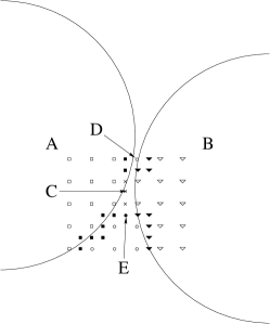
Figure 1: The blank squares and triangles depict the inner fluid of particles A and B respectively. The filled squares and triangles denote the discretized surface; fluid particles crossing that surface are reflected. The empty circles represent the outer fluid, while crosses (C) denote the shared boundary nodes. The filled circle E is not a real shared node, but belongs to both spheres (A and B), although it lies on different links. D is a single outer node between the two surfaces. If those surfaces move towards each other, high pressure occurs at D.

To simulate the hydrodynamic interactions between solid particles in suspensions, the lattice-Boltzmann model has to be modified to incorporate the boundary conditions imposed on the fluid by the solid particles. Stationary solid objects are introduced into the model by replacing the usual collision rules (Eq. (6)) at a specified set of boundary nodes by the “link-bounce-back” collision rule N.-Q. Nguyen and A.J.C. Ladd (2002). When placed on the lattice, the boundary surface cuts some of the links between lattice nodes. The fluid particles moving along these links interact with the solid surface at boundary nodes placed halfway along the links. Thus, a discrete representation of the surface is obtained, which becomes more and more precise as the surface curvature gets smaller and which is exact for surfaces parallel to lattice planes. Two discretized spherical surfaces near contact are shown as filled symbols in Fig. 1. Empty symbols denote the fluid, while filled squares and triangles depict the discretized surface. The crosses (C) denote the shared boundary nodes in contrast to the filled circle (E) which is not a shared boundary node since it is placed on individual links for each sphere.

Numerical results of simulations of a stationary Poisseuille-flow between two flat surfaces are in good agreement with the theoretical formula L.D. Landau and E.M. Lifschitz (1966)

$$v=\frac{gL^{2}}{12\eta}\left(1-\frac{4(x-L)^{2}}{L^{2}}\right).$$ (11)

This is demonstrated in figure 2 which shows the velocity profile vs. dimensionsless distance $x/L$ from the left wall of a fluid with viscosity $\eta=\frac{1}{9}$ and density $\rho=1$ under constant force $g$ exerted on each lattice point in a channel with width $L$. $g$ is set to $10^{-4}$ for $L\in\{8;16;32\}$ and to $g=5\times 10^{-5}$ for $L=16$. $\eta,g,\rho,L$ are in lattice units. The solid line corresponds to the profile as expected from Eq. (11).

Figure 2: Poisseuille-flow of a fluid with viscosity $\eta=\frac{1}{9}$ and density $\rho=1$ under gravity $g=10^{-4}$ exerted on each lattice point, channel width $L\in\{8;16;32\}$. Gravity is set to $g=5\times 10^{-5}$ for channel width $L=16$. The solid line represents the expected profile (Eq. (11)).

Since the velocities in the lattice-Boltzmann model are discrete, boundary conditions for moving suspended particles cannot be implemented directly. Instead, we can modify the density of returning particles in a way that the momentum transferred to the solid is the same as in the continuous velocity case. This is implemented by introducing an additional term $\Delta_{b}$ in Eq. (2) Ladd (1994a):

$$\Delta_{b,i}=\frac{2\omega^{c_{i}}\rho_{i}{\mathbf{u}}_{i}\cdot{\mathbf{c}}_{i}}{c_{s}^{2}},$$ (12)

with $c_{s}$ being the velocity of sound and coefficients $\omega^{c_{i}}$ from Eq. (8).

To avoid redistributing fluid mass from lattice nodes being covered or uncovered by solids, we allow interior fluid within closed surfaces. Its movement relaxes to the movement of the solid body on much shorter time scales than the characteristic hydrodynamic interaction Ladd (1994a). Fig. 3 shows a cut through a three-dimensional box containing a sphere $S$ with periodic boundaries on front, back, left and right sides. On the top and bottom sides as well as on the sphere surface we use link-bounce-back boundary conditions. The particle is falling under the influence of gravity $g$. The system size is $32\times 32\times 32$ lattice constants $a$ and the particle radius is $4a$. At the beginning the particle and the fluid are at rest and after 3000 time steps the particle attains a steady state. The cut in Fig. 3 has been generated after 5155 time steps, i.e. well after the system has reached the steady state. Its velocity $u$ is 19% higher than $u_{\infty}$, expected by Stokes’ equation in an inifinite fluid system L.D. Landau and E.M. Lifschitz (1966). The difference is caused by the fluid vortices $V$ seen in Fig. 3, which is due to the periodic boundary conditions and could not arise in an infinite system.

Figure 3: Cut through a three-dimensional system after 5155 time steps. The link-bounce-back boundary conditions are implemented on the surface of the sphere and the walls. The particle Reynolds number is $\mathrm{Re}=6$ and ${\mathbf{g}}$ is the gravitational force. The movement of the interior fluid has already relaxed to solid body movement.

II.3 Boundary nodes shared between two particles

If two particle surfaces approach each other within one lattice spacing, no fluid nodes are available between the solid surfaces (Fig. 1). In this case, mass is not conserved anymore since boundary updates at each link produce a mass transfer $\Delta_{b}a^{3}$ ($a\equiv$cell size) across the solid-fluid interface Ladd (1994a). The total mass transfer for any closed surface is zero, but if some links are cut by two surfaces, no solid-fluid interface is available anymore. Instead, the surface of each particle is not closed at the solid-solid contacts anymore and mass can be transferred in between suspended particles. Since fluid is constantly added or removed from the individual particles, they never reach a steady state. In such cases, the usual boundary-node update procedure is not sufficient and a symmetrical procedure which takes account of both particles simultaneously has to be used Ladd (1994b). Thus, the boundary-node velocity is taken to be the average of that computed from the velocities of each particle. Using this velocity, the fluid populations are updated (Eq. (12)), and the force is computed; this force is then divided equally between the two particles.

II.4 Lubrication interactions

If two particles are in near contact, the fluid flow in the gap cannot be resolved by LB. For particle sizes used in our simulations ($R<5a$), the lubrication breakdown in the calculation of the hydrodynamic interaction occurs at gaps less than $0.1R$ N.-Q. Nguyen and A.J.C. Ladd (2002). This effect ”pushes“ particles into each other.

To avoid this force, which should only occur on intermolecular distances, we use a lubrication correction method described in Ref. N.-Q. Nguyen and A.J.C. Ladd (2002). For each pair of particles a force

$${\mathbf{F}}_{\text{lub}} =-6\pi\eta\frac{R_{1}R_{2}}{(R_{1}+R_{2})^{2}}\left(\frac{1}{h}-\frac{1}{h_{N}}\right){\mathbf{u}}_{12}\cdot\frac{{\mathbf{r}}_{12}}{\lvert{\mathbf{r}}_{12}\rvert}, h<h_{N}$$ (13)

is calculated, where ${\mathbf{u}}_{12}={\mathbf{u}}_{1}-{\mathbf{u}}_{2},h=\lvert{\mathbf{r}}_{12}\rvert-R_{1}-R_{2}$ is the gap between the two surfaces and a cut off distance $h_{N}=\frac{2}{3}a$ A.J.C. Ladd and R. Verberg (2001). For particle-wall contacts we apply the same formula with $R_{2}\rightarrow\infty$ and $h=\lvert{\mathbf{r}}_{12}\rvert-R_{1}$. The tangential lubrication can also be taken into account, but since it has a weaker logarithmic divergence and its breakdown does not lead to serious problems, we do not include it in our simulations.

This divergent force can temporarily lead to high velocities, which destabilize the LB scheme. Instabilities can be reduced by averaging the forces and torques over two successive time steps Ladd (1994b). In Ref. C.P. Lowe et al. (1995) an implicit update of the particle velocity was proposed. This method then has been generalized and adopted for LB where two particles are in near contact A.J.C. Ladd and R. Verberg (2001); N.-Q. Nguyen and A.J.C. Ladd (2002). The drawback of this algorithm is the requirement of two sweeps over all boundary nodes. As we study creeping motion, we use the following simple method. High forces can only arise if the lubrication correction is switched on. Therefore, the lubrication correction ${\mathbf{F}}_{\text{lub}}$ is limited to a value which would cause a particle acceleration of $0.1$ Mach/s. Such a limitation may lead to particle overlap, but we found that on average there are only 5 occurences of this limitation per particle within $10^{6}$ time steps.

II.5 Particle motion

The particle position and velocity is calculated using Newton’s equations

$${\mathbf{a}} =\frac{1}{m}{\mathbf{F}}=\dot{{\mathbf{v}}}, {\mathbf{v}}=\dot{{\mathbf{r}}}.$$ (14)

The force ${\mathbf{F}}$ is obtained from the calculation of the particle-fluid coupling and the lubrication corrections. Then, the equations are discretized and integrated using the Euler-Cromer method Giordano (1997). The velocity ${\mathbf{v}}_{n+1}$ and position ${\mathbf{r}}_{n+1}$ for the time step $n+1$ are obtained by utilizing the velocity, position and force from time step $n$ as well as the time step $\Delta t=1$ and particle mass $m$.

$${\mathbf{v}}_{n+1} ={\mathbf{v}}_{n}+\frac{{\mathbf{f}_{n}}}{m}\Delta t$$ (15a)

$${\mathbf{r}}_{n+1} ={\mathbf{r}}_{n}+{\mathbf{v}}_{n+1}\Delta t$$ (15b)

The same method is applied to particle rotation, with position replaced by angles, velocity by angular velocity, force by torque and mass by moment of inertia. We do not use more sophisticated methods since they either require additional memory and extra calculations (Verlet M. P. Allen and D. J. Tildesley (1987), Runge-Kutta W.H. Press et al. (2002)) or require the solution of an implicit equation for the velocity at each particle boundary node (Velocity-Verlet) W.C. Swope et al. (1982). Since the forces and velocities in our simulation are rather small and the particle kinetic energy is not conserved between collisions (it is changed by particle-fluid interaction), we do not need to care for neglegible numerical inaccuracies of this method.

III Simulations

The purpose of our simulations is the reproduction of rheologic experiment on computers. First, we simulate a representative volume element of the experimental setup. Then we can compare our calculations with experimentally accessible data, i.e. density profiles, time dependence of shear stress and shear rate. We also get experimentally inaccessible data from our simulations like translational and rotational velocity distributions, particle-particle and particle-wall interaction frequencies.

The experimental setup consists of a rheoscope with two spherical plates, which distance can be varied. The upper plate can be rotated either by exertion of a constant force or with a constant velocity, while the complementary value is measured simultaneously. The material between the rheoscope plates consist of glass spheres suspended in a sugar-water solution. The radius of the spheres varies between $75$ and $150$ $\mu$m. For our simulations we assume an average particle radius of 112.5 $\mu$m. The density and viscosity of the sugar solution can also be changed.

Because glass and suger solution have different light absorption constants, the particle concentration can be obtained by spectroscopic methods. Alternatively, the experimental material can be frozen and analyzed by an NMR spectroscope and a three dimensional porosity distribution can be extracted from the data. Details of the experiment which is currently under development can be found in S. Muckenfuß and H. Buggisch (2003); Buggisch (1995, 1997); H. Buggisch and G. Barthelmes (1998).

A low resolution ($R\sim 2a$) simulation of a system with the same volume as the experiment would need about 10 GB RAM which is about five times as much as typically available in current workstations. Each time step the program sweeps at least twice over the full data set. Simulating one minute real time would need about three years CPU time. Increasing the resolution or implementing curved boundary would increase the computation time even more. Therefore, we calculate only the behavior of a representative volume element which has the experimental separation between walls, but a much lower extension in the other two dimensions than the experiment. In these directions we employ periodic boundary conditions for particles and for the fluid.

Shearing is implemented using the “link-bounce-back” rule with an additional term $\Delta_{b,i}$ at the wall in the same way as already described for particles (Eq. (12) with ${\mathbf{u}}_{i}$ now being the velocity of the wall). If a fluid node between the particle and the wall is missing, we use the approach for shared boundary nodes as discussed in section II.3.

To compare the numerical and experimental results, we need to find characteristic dimensionless quantities of the experiment which then determine the simulation parameters. For this purpose we use the ratio of the rheoscope height and the particle size $\lambda$, the particle Reynolds number $\mathrm{Re}$ and the volume fraction of the particles $\phi$:

$$\lambda =\frac{R}{L}, \mathrm{Re} =\frac{\gamma R^{2}\rho_{f}}{\eta}, \phi =\frac{N\cdot\frac{4}{3}\pi R^{3}}{V_{s}},$$ (16)

with $R$ being the particle radius, $L$ the height of the rheoscope, $\gamma$ the shear rate, $\eta$ the fluid viscosity and $N$ the number of particles. In the experiment the suspended particles have a slightly lower density than the fluid. Reducing the particle density would cause instabilities in LB. Therefore, we need to change the acceleration of gravity to a value, which would cause the same sedimentation or buoyancy velocity $u$. Stokes’ law L.D. Landau and E.M. Lifschitz (1966) gives the connection between $u$ and gravity $g$:

$$F =6\pi R\eta u \Leftrightarrow u =\frac{mg}{6\pi R\eta},$$ (17)

with the effective mass $m=\frac{4}{3}\pi R^{3}(\rho_{s}-\rho_{f})$ of the solid particle. Converting $u$ to the dimensionless velocity $u^{\prime}$ (lattice constant/time step) and inserting simulation parameters into the last equation we get

$$g^{\prime}=\frac{6\pi R^{\prime}\eta^{\prime}u^{\prime}}{m^{\prime}},$$ (18)

where $m^{\prime}$ is the mass of the particle without interior fluid, $R^{\prime}$ the particle radius and $\eta^{\prime}$ the fluid viscosity (Eq. (9)).

To provide the simulation results with units, we calculate the length of the lattice constant $a=R/R^{\prime}$ and the duration of one time step $\Delta t=\gamma^{\prime}/\gamma$: Using $R=1.125\cdot 10^{-4}$ m, $L=3.375\cdot 10^{-3}$ m, $\rho_{f}=1446$ $\frac{\text{kg}}{\text{m}^{3}}$, $\rho_{s}=1180$ $\frac{\text{kg}}{\text{m}^{3}}$, $\eta=0.450$ $\frac{\text{kg}}{\text{m}\cdot\text{s}}$, $\gamma=10\text{ s}^{-1}$, $R^{\prime}=\frac{59}{30}$, $L=59$, $\nu^{\prime}=\frac{1}{9}$ and $\rho_{f}^{\prime}=0.7$ we obtain

$$a =0.572\cdot 10^{-4}\text{ m}, \Delta t =1.262\cdot 10^{-4}\text{ s}.$$ (19)

In the simulations presented in the next section we vary the particle Reynolds number to find the dependence of the time needed to attain a steady state and strength of structuring effects on the shear rate.

Next we vary the particle volume fraction to study the correlation of velocity profiles and particle concentration. Different volume fractions lead to different correlation effects of particle positions and density profiles.

To check our conversion rule between numerical and experimental data, we will try to change the fluid viscosity without changing the Reynolds number. This leads to different shear rates and consequently different time steps in the simulation. Higher viscosities lead to longer time steps and thus to shorter simulation times.

A system with $\mathrm{Re}=4\cdot 10^{-6}$ needs about $900\text{ s}$ to attain the steady state. $900\text{ s}$ are equivalent to $7\cdot 10^{6}$ iterations. For such a high number of iterations the program requires about 20 CPU-days on a 2 GHz AMD Opteron.

IV Results

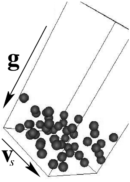
Figure 4: A snapshot of a suspension with 50 spheres (radius $R=1.125\cdot 10^{-4}\text{ m}$, mass $m=7.7\cdot 10^{-8}\text{ kg}$) at time $t=729\text{ s}$ which corresponds to 5772500 time steps. The volume of the simulated system is $1.83\cdot 10^{-3}\times 1.83\cdot 10^{-3}\times 3.375\cdot 10^{-3}\text{ m}=11.3025\cdot 10^{-9}\text{ m}^{3}$, acceleration of gravity $g=0.80\text{ m/s}^{2}$, and shear velocity $v_{s}=3.375\cdot 10^{-2}\text{ m/s}$. The fluid has a viscosity $\eta=450\text{ mPa}\cdot\text{s}$ and density $\rho_{f}=1446\frac{\text{kg}}{\text{m}^{3}}$. This visualization is a typical example for a system that has reached a steady state: All particles have fallen to the ground due to the exerted gravitational force and most of the system has no particles.

Fig. 4 shows a snapshot of a suspension with 50 spheres after $5772500$ time steps which are equivalent to $729\text{ s}$. The vector ${\mathbf{g}}$ represents the direction of gravity and ${\mathbf{v}}_{S}$ depicts the velocity of the sheared wall.

The particles feel a gravitational acceleration $g=0.8\text{ m/s}^{2}$, have a mass $m=7.7\cdot 10^{-8}\text{ kg}$, a Reynolds number $\mathrm{Re}=4.066875\cdot 10^{-4}$, and a radius $R=1.125\cdot 10^{-4}\text{ m}$. The system size is $1.83\cdot 10^{-3}\times 1.83\cdot 10^{-3}\times 3.375\cdot 10^{-3}\text{ m}$ which corresponds to a lattice size of $32\times 32\times 59$. The density of the fluid is set to $\rho_{f}=1446\frac{\text{kg}}{\text{m}^{3}}$ and its viscosity is $\eta=450\text{ mPa}\cdot\text{s}$. The walls at the top and the bottom are sheared with a relative velocity $v_{s}=3.375\cdot 10^{-2}\text{ m/s}$. The system size, particle size and mass, as well as the gravitational force and all fluid parameters are fixed throughout the paper. After 200 time steps a linear fluid velocity profile can be observed and the particles are inserted in a random fashion: After choosing a random position for the particle, we check if the distance between these coordinates and the centers of all other spheres is at least $2R+a$ in order to avoid high interparticle forces. The initial particle velocities are set to the velocity of the fluid at the center of the particles. This algorithm allows a dense and uniform particle distribution within the whole simulation volume and has been applied in all our simulations. Fig. 4 is a representative visualization of our simulation data and demonstrates that after the system has reached its steady state, all particles have fallen to the ground due to the influence of the gravitational force. Most of the simulation volume is free of particles.

Figure 5: Density profiles from simulations with two different shear rates $\gamma=10\text{ s}^{-1}$ (a) and $\gamma=1\text{ s}^{-1}$ (b). Other parameters are equal to those given in Fig. 4. (a) shows five peaks with separations about one particle diameter, which reveal the forming of particle layers. The number of particles per layer is decreasing with increasing distance to the wall, and the change in particle numbers is caused by gravity which is directed perpendicular to the wall at $z=0$. Although we used the same gravity and particle numbers, there are only three peaks in (b) and their width is higher than in (a), demonstrating that the structuring effects strongly relate to the shear rate.

In order to quantitatively characterize structuring effects, we calculate the particle density profile of the system by dividing the whole system into layers parallel to the walls and calculating a partial volume $V_{ij}$ for each particle $i$ crossing such a layer $j$. The scalar $V_{ij}$ is given by the volume fraction of particle $i$ that is part of layer $j$:

$$V_{ij}=\pi\left(R^{2}\left(R_{ij}^{\text{max}}-R_{ij}^{\text{min}}\right)-\frac{1}{3}\left(R_{ij}^{\text{max}}-R_{ij}^{\text{min}}\right)\right)$$ (20)

If the component $r_{i,z}$ perpendicular to the wall of the radius vector ${\mathbf{r}}_{i}$ of the center of sphere $i$ lies between $r_{j}^{\text{min}}$ and $r_{j}^{\text{max}}$, we have

$$r_{j}^{\text{min}} =\left(j-\frac{1}{2}\right)\Delta L_{z}-R,$$

$$r_{j}^{\text{max}} =\left(j+\frac{1}{2}\right)\Delta L_{z}+R,$$

and

$$R_{ij}^{\text{max}} =\left\{\begin{array}[]{ll}R&\text{if }r_{i,z}+R<r_{j}^{\text{max}}\\ r_{j}^{\text{max}}-r_{i,z}&\text{else}\\ \end{array}\right.,$$ (23)

$$R_{ij}^{\text{min}} =\left\{\begin{array}[]{ll}-R&\text{if }r_{i,z}-R>r_{j}^{\text{min}}\\ r_{j}^{\text{min}}-r_{i,z}&\text{else}\\ \end{array}\right..$$ (26)

Finally, the sum of all weights associated with a layer is divided by the volume of the layer

$$\phi_{j} =\frac{1}{L_{x}\cdot L_{y}\cdot\Delta L_{z}}\sum\limits_{i=1}^{N}v_{ij}, \Delta L_{z} =\frac{L_{z}}{M},$$ (27)

with $L_{x},L_{y}$ being the system dimensions between periodic boundaries, $L_{z}$ the distance between walls, $M$ the number of layers, and $\Delta L_{z}$ the width of a single layer.

Density profiles calculated by this means for systems with two different shear rates $\gamma=10\text{ s}^{-1}$ and $\gamma=1\text{ s}^{-1}$ are presented in Fig. 5. All other parameters are equal to the set given in the last paragraph. The peaks in Fig. 5 demonstrate that at certain distances from the wall the number of particles is substantially higher than at other positions. The first peak in both figures is slightly below one particle diameter, which can be explained by a a lubricating fluid film between the first layer and the wall which is slightly thinner than one particle radius. Due to the small amount of particles, time dependent fluctuations of the width of the lubricating layer cannot be neglected and a calculation of the exact value is not possible. The five peaks in Fig. 5a have samilar distances which are equal to one particle diameter. These peaks can be explained by closely packed parallel layers of particles. Due to the linear velocity profile in $z$ direction of the fluid flow, every layer adopts the local velocity of the fluid resulting in a relative velocity difference between two layers of about $2R\gamma$. These layers stay stable in time with only a small number of particles being able to be exchanged between them.

Fig. 5b only shows three peaks with larger distances than in Fig. 5a. However, the average slope of the profile is identical for both shear rates. For smaller shear rates, velocity differences between individual layers are smaller, too. As a result, particles feel less resistance while moving from one layer to another. Every inter-layer transition destorts the well defined peak structure of the density distribution resulting in only three clearly visible peaks in Fig. 5b.

With changing time, the first peak stays constant for both shear rates. The shape, number and position of all other peaks is slightly changing in time.

To aquire a quantitative description of ths effect we calculate the autocorrelation function of the density profile (Fig. 6) $r_{\tau}^{l}$ for each individual layer $l$,

$$r_{\tau}^{l}(i\cdot\Delta t)=\frac{\frac{1}{(T-i)}\sum\limits_{j=1}^{T-i}\phi^{l}(j\cdot\Delta t)\cdot\phi^{l}((i+j)\Delta t)}{\frac{1}{T}\sum\limits_{j=1}{T}\left(\phi^{l}(j\cdot\Delta t)\right)^{2},}$$ (28)

with $\Delta t$ being the time step, $i$ the current iteration and $T$ the total number of time steps.

Figure 6: Autocorrelation $r_{\tau}$ of the density profiles shown in Fig. 5. In both plots the autocorrelation converges to a fixed value. The dashed lines correspond to fitted constants and the points to the simulation data. In (a) the system has a shear rate $\gamma=10\text{ s}^{-1}$ and in (b) $\gamma=1\text{ s}^{-1}$. The higher shear rate leads to higher particle velocities and therefore to a higher collision frequency. Therefore, this system faster attains the steady state and is less correlated. This is confirmed by the smaller limit of $r_{\tau}$, which is $0.361$ instead of $0.480$ in (b).

Averaging the $r_{\tau}^{l}$ over all $M$ layers gives

$$r_{\tau}(i\cdot\Delta t)=\frac{1}{M}\sum\limits_{l=1}^{M}r_{\tau}^{l}(i\cdot\Delta t),$$ (29)

which is presented in Fig. 6 for two systems with shear rates $\gamma=10\text{ s}^{-1}$ and $\gamma=1\text{ s}^{-1}$. The autocorrelation starts — as given by definition — at one. Then, it decreases and converges to constant values at about $i\cdot\Delta t=15\text{ s}$ for $\gamma=10\text{ s}^{-1}$ and at $i\cdot\Delta t=25\text{ s}$ for $\gamma=1\text{ s}^{-1}$. We obtain these values by fitting the data to a constant function using a nonlinear least-squares Marquardt-Levenberg algorithm. The computed values of the autocorrelation function are different for the given shear rates: $r_{\tau}$ is $0.480$ for $\gamma=1\text{ s}^{-1}$ and $0.361$ for $\gamma=10\text{ s}^{-1}$ respectively. It is evident that for a simulation without shear the autocorrelation converges to one because after sedimentation the density profile should not change. Thus, $\phi^{l}(k\cdot\Delta t)$ is almost constant for all $k$, and $r_{\tau}\rightarrow\infty$. For $\gamma\rightarrow\infty$ the velocity and the collision frequency are increasing and the correlation decreases for high shear rates. Therefore, the expectation that for smaller shear rates the autocorrelation converges to higher values than for larger shear rates, is confirmed.

Another possibility to compute typical correlation times of structured layers is to analyze the autocorrelation of particle distances to one of the walls. For this purpose we replace the volume fraction $\phi^{l}(k\cdot\Delta t)$ of layer $l$ by the distance of particle $l$ to one of the walls $r^{l}_{z}$ in Eq. (28). Then the acquired data is averaged for all $N$ particles

$$r_{\tau}(i\cdot\Delta t)=\frac{1}{N}\sum\limits_{l=1}^{N}r_{\tau}^{l}(i\cdot\Delta t).$$ (30)

The dependence of $r_{\tau}$ on time calculated by this means is shown in Fig. 7, where simulation parameters are as in the previous section.

Figure 7: Autocorrelation $r_{\tau}$ of the particle distances from a wall for two systems with shear rates $\gamma=10\text{ s}^{-1}$ (a) and $\gamma=1\text{ s}^{-1}$ (b). All simulation parameters exept $\gamma$ correspond to those given in Fig. 4. The straight line in the plots with logarithmically scaled $r_{\tau}$-axes shows the exponential connection of $r_{\tau}$ and time $t$: $r_{\tau}\propto e^{-t/\tau_{\text{corr}}}$. The typical correlation time $\tau$ evidently depends on the shear rate. We find $\tau_{\text{corr}}=5.5\text{ s}$ and $\tau_{\text{corr}}=38.64\text{ s}$ for $\gamma=10\text{ s}^{-1}$ and $\gamma=1\text{ s}^{-1}$ respectively.

It is possible to fit the data to an exponential function of the form

$$r_{\tau}=e^{-\frac{t}{\tau_{\text{corr}}}},$$ (31)

where $\tau_{\text{corr}}$ is the characteristic correlation time. We get $\tau_{\text{corr}}=5.5\text{ s}$ and $\tau_{\text{corr}}=38.64\text{ s}$ for $\gamma=10\text{ s}^{-1}$ and $\gamma=1\text{ s}^{-1}$, respectively. This fully corresponds to the behavior expected from the density profiles: Shorter correlation times are related to higher shear rates. At higher shear rates the mean velocity of the particles is also higher. Thus they collide with other particles and walls more often. Each collision contributes a random uncorrelated force component to the equation of motion, which reduces the correlation of particle positions.

We also expect a strong dependence on the average particle concentration and different values for the gravitational force. For a larger number of particles in the system, the effective viscosity changes which influences the collision rate and reduces correlation times.

Also for very high shear rates there should be nonzero correlation times, and we expect a non-linear connection between shear rate and correlation time.

Figure 8: Dependency of the correlation time $\tau_{\text{corr}}$ on the shear rate $\gamma$. All data points lie on a straight line, which indicates an exponential behaviour of $\tau_{\text{corr}}$: $\tau_{\text{corr}}\propto e^{-\gamma/\gamma_{0}}$, with $\gamma_{0}=4.78\text{ s}^{-1}$.

Therefore, we did the same calculations for more different shear rates and plot the correlation times $\tau_{\text{corr}}$ versus shear rates $\gamma$ in Fig. 8. Rescaling the axis of ordinates logarithmically we obtain a straight line again. For high shear rates the correlation time is decreasing exponentially:

$$\tau_{\text{corr}}=\tau_{\text{corr}}^{\text{max}}\cdot e^{-\frac{\gamma}{\gamma_{0}}},$$ (32)

with $\tau_{\text{corr}}^{\text{max}}=47.24\text{ s}$ being the maximum correlation time and $\gamma_{0}=4.78\text{ s}^{-1}$ being a characteristic shear rate.

Figure 9: Distributions of particle distances (a) and of differences of particle distances to one of the walls (b). All simulation parameters are equal to those given in Fig. 4. In both figures we show histograms for two different times: $t=0\text{ s}$ and $t=865\text{ s}$. In (a) the dominant peak moves from $\delta\sim 1.2$ to $\delta\sim 1$ showing the compression of the system under the influence of gravity. There is also a shoulder on the right of the peak showing that many particles have distances between $1$ and $2$ particle radii. In (b) we see a linear profile for $t=0$, caused by the homogeneous particle distribution at the beginning of the simulation. The highest peak is at $\delta=0$, which is caused by particles belonging to identical layers. The following peak is due to particles from adjacent layers.

Another interesting property is the distribution of particle distances, which can be acquired by calculating the distances $r(i,j,l)$ of all particle pairs. Because of periodic boundary conditions we also account for particle pairs if one of them is shifted in one of the nine possible periodic directions. The maximum distance is then limited by the smallest system dimension $L_{\text{min}}$ (here $1.83\cdot 10^{-3}\text{ m}$).

$$p_{k}=\frac{1}{N^{\prime}}\sum\limits_{i=1}^{N}\sum\limits_{j=i+1}^{N}\sum\limits_{l=1}^{9}\left\{\begin{array}[]{ll}\frac{1}{\delta^{2}}&\text{if }\left[\frac{r(i,j,l)}{\Delta r}\right]=k\\ 0&\text{else}\\ \end{array}\right.,$$ (33)

with

$$\Delta r=\frac{L_{\text{min}}}{M},$$

$$N^{\prime}=\sum\limits_{i=1}^{N}\sum\limits_{j=i+1}^{N}\sum\limits_{l=1}^{9}\left\{\begin{array}[]{ll}1&\text{if }r(i,j,l)<L_{\text{min}}\\ 0&\text{else}\\ \end{array}\right.,$$

$$r(i,j,l)=\lvert{\mathbf{r}}_{i}-({\mathbf{r}}_{j}+{\mathbf{s}}_{l})\rvert,$$

$${\mathbf{s}}_{l}=\begin{pmatrix}0\\ 0\\ 0\\ \end{pmatrix},\begin{pmatrix}\pm L_{x}\\ 0\\ 0\\ \end{pmatrix},\begin{pmatrix}0\\ \pm L_{y}\\ 0\\ \end{pmatrix},\begin{pmatrix}\pm L_{x}\\ \pm L_{y}\\ 0\\ \end{pmatrix}.$$

Each $p_{k}$ corresponds to an inter-particle distance

$$\delta=\left(k+\frac{1}{2}\right)\Delta r.$$ (34)

In a homogeneous system the number of particles with a distance $\delta$ to a given particle is proportional to the surface of a sphere of radius $\delta$. Thus to avoid overweighting of larger particle distances we divide the number of particles with distance $\delta$ by $\delta^{2}$ (Eq. (33)).

In Fig. 9a we present two distributions for a system with $50$ particles. The first distribution corresponds to the start of the simulation at $t=0\text{ s}$. It has one peak between $\delta=1$ and $\delta=2$, after which it decreases continuously. The measurement in steady state gives the second distribution at $t=865\text{ s}$. This distribution also has one peak, but it is narrower and much higher than at $t=0\text{ s}$. The position of this peak corresponds to a distance $\delta$ slightly higher than $1$ particle diameter to each other, i.e. most particles have a distance of about one particle diameter.

By computing only the distribution of the components of particle distances perpendicular to the walls $r_{z}$ for the same system we get the results plotted in Fig. 9b. We do not need to account for periodic boundaries here resulting in a smaller number of counted particle pairs and slightly worse statistics:

$$p_{k}=\frac{2}{N(N-1)}\sum\limits_{i=1}^{N}\sum\limits_{j=i+1}^{N}\left\{\begin{array}[]{ll}1&\text{if }\left[\frac{r_{z}(i,j)}{\Delta r}\right]=k\\ 0&\text{else}\\ \end{array}\right.,$$ (35)

with $N$ being the number of particles in the system, and

$$r_{z}(i,j) =\lvert r_{zi}-r_{zj}\rvert, \Delta r =\frac{L_{\text{z}}}{M},$$ (36)

where $M$ is the resolution of the distribution, $L_{\text{z}}$ the distance between the walls, and $\delta$ is calculated as given in Eq. (34). The distributions in Fig. 9b show that for $t=0\text{ s}$ there are no structured layers. This histogram gives a nearly straight line with a negative slope.

Let us consider a homogeneous system completely filled with spheres and $x$ being the number of particles in an individual layer. Then, $x(x-1)$ is the number of particle pairs with distance $\delta=L_{z}-1$. For $\delta=L_{z}-2$ there are two pairs of layers of that distance. Thus, we get $2x(x-1)$ particle pairs. Reducing the distance by one particle diameter increases the number of possible particle pairs by $x(x-1)$. The total number of particle pairs is propotional to $L_{z}-\delta$. This argumentation is valid for all homogenously filled systems. This consideration is comfirmed by Fig. 9b for $t=0$. The slope of the line should be propotional to the volume fraction because $x$ gets larger for higher particle numbers. After $865\text{ s}$ there is a peak for $\delta=0$ showing that most pairs belong to the same layer. The second peak belongs to $\delta\sim 1$, i.e. to particle pairs at adjacent layers.

Figure 10: The mean $\langle\delta\rangle$ and standard deviation $\sigma$ of particle distances (a) and differences of particle distances to one of the walls (b) versus time for a system of $50$ particles with radius $R=1.125\cdot 10^{-4}\text{ m}$, acceleration of gravity $g=0.80\text{ m/s}^{2}$. The Reynolds number is Re $=4.066875\cdot 10^{-4}$, and the shear rate $\gamma=10\text{ s}^{-1}$. In both figures $\langle\delta\rangle$ and $\sigma$ converge to specific values within ca. $15\text{ s}$ and they fluctuate around fixed values till the end of the simulation ($t\simeq 900\text{ s}$). In both cases the standard deviation is smaller than the mean. The mean particle distance converges to $\langle\delta\rangle\simeq 4.6$ and its standard deviation converges to $\sigma\simeq 3.2$. The mean difference of particle distances to the wall converges to $\langle\sigma\rangle\simeq 1.2$ and $\sigma\simeq 1$.

Both histograms in Fig. 9 have a clear dependence on time. To visualize that dependence we calculate the mean $\langle\delta\rangle$ and standard deviation $\sigma$ of particle distances.

$$\langle\delta\rangle =\frac{1}{M}\sum\limits_{i=1}^{M}p_{i}\cdot\delta_{i},$$ (37a)

$$\sigma =\sqrt{\frac{1}{M}\sum\limits_{i=1}^{M}p_{i},\cdot\left(\delta_{i}-\langle\delta\rangle\right)^{2}},$$ (37b)

$$\delta_{i} =\frac{i\cdot\delta_{\text{max}}}{M},$$

with $M$ being the resolution of the distribution $p(\delta)$, and $\delta_{\text{max}}$ being the maximum particle distance. For the distribution of differences of particle distances to one of the walls $\delta_{\text{max}}$ is set to $3.375\cdot 10^{-3}\text{ m}\equiv 15\text{ particle diameters}$. For the distribution of particle distances $\delta_{\text{max}}=1.8\cdot 10^{-3}\text{ m}\equiv 8.136\text{ particle diameters}$. In Fig. 10a the mean $\langle\delta\rangle$ (left ordinate) and $\sigma$ (right ordinate) are plotted over time. For short times, the mean decreases almost linearly to $t\sim 16\text{ s}$, then the slope approaches $0$ and $\langle\delta\rangle$ fluctuates around $\delta=4.65$ till the end of the simulation ($t\sim 900\text{ s}$). At the beginning of the simulation it is not possible to recognise the characteristics of the evolution of $\sigma$. For times between $6$ and $15\text{ s}$ the points of $\sigma$ lie nearly on a straight line. At $t\sim 16$ the slope of $\sigma$ becomes zero and $\sigma$ is fluctuating around a mean $\sigma=3.2$ like $\langle\delta\rangle$.

In Fig. 10b the mean $\langle\delta\rangle$ and standard deviation $\sigma$ of differences of particle distances to one of the walls are plotted versus time. To calculate these values we used the equations (37). The evolution of $\langle\delta\rangle$ and $\sigma$ is nearly linear between $t=5\text{ s}$ and $t=12\text{ s}$. The slope then vanishes and only some random fluctuations can be seen around $\langle\delta\rangle=1.4$ and $\sigma=1.2\text{ particle diameters}$ for $t\geq 17\text{ s}$. Note that the particle distances attain a steady state already after $15\text{ s}$ while the density profile needs $158\text{ s}$.

Figure 11: Velocity profile of a system with shear rate $\gamma=10\text{ s}^{-1}$ and mean volume fraction $\phi=0.026$ versus distance to one of the walls $z$. Solid lines correspond to the expected fluid velocity profile in absence of particles. At the walls ($z=0$ and $z=15$), the fluid velocity is identical to the wall velocities and in the particle filled region the fluid and solid velocities are equal confirming the validity of the no-slip boundary conditions on particle and wall surfaces. The velocity of the solid particles does not disappear at the wall unlike the fluid velocity, but converges to a fixed value instead.

To study the demixing phenomena already demonstrated in Fig. 5, we analyze the dependency of the particle and fluid velocities on the distance to the wall. Both profiles in Fig. 11 are for a system with shear rate $\gamma=10\text{ s}^{-1}$ at $t=865\text{ s}$. All other simulation parameters are kept as in the last section. In addition to the velocity profiles we plot a solid line corresponding to the fluid velocity profile of a system without particles. The values of fluid velocities at the walls ($z=0$ and $z=15$ particle diameters) exactly match the wall velocities: $v(0)=0$ and $v(15)=3.375\cdot 10^{-2}\text{ m/s}$. For $2<z<6$ both profiles agree very well with each other. No particles are present above $z=6$ and the fluid velocity profile is exactly linear. We do not have any particle velocity data in this case. Below $z=2$ the profiles separate and for $z<0.5$ the fluid velocity profile corresponds to the expected profile for a particle free system, while the particle velocities stay constant. This can be seen in Fig. 11b, which shows an enlarged particle velocity profile. The particle velocity converges to $v_{s}=1.1\cdot 10^{-3}\text{ m/s}$ for $z\rightarrow 0$. For higher values of $z$ it is linear, but its slope is about 10% smaller than the slope of the solid line. For $z>6$ the velocity profile is linear, but it raises faster than expected in order to fit the wall velocity at $z=15$ and to conserve the validity of the no-slip boundary conditions at the walls. Since the particle and fluid velocities are identical for $2<z<6$, the no-slip boundary conditions on the particle surface are shown to generate correct results, too.

Figure 12: The velocity of the “pseudo-wall-slip” versus shear rate for two different volume concentrations. The dependence of the velocity is linear. The slope of the line gives an effective width of the particle free region near the wall. The width is $1.16\cdot 10^{-4}\text{ m}$ and $9.23\cdot 10^{-5}\text{ m}$ for $\phi=0.026$ and $\phi=0.053$, respectively. Narrower particle free regions are caused by higher forces due to weight of particles being above the particle layer near the wall.

The dependence of the particle velocity near the wall on the shear rate is studied in Fig. 11b for $\gamma=1,0.1,$ and $0.25\text{ s}^{-1}$ by calculating the particle velocities for $z\rightarrow 0$. Fig. 12 depicts these velocities versus shear rate and their linear dependence is clearly observable. The data from simulations with higher particle concentration ($\phi=0.053$ instead of $\phi=0.026$) also gives a straight line but with smaller slope. The slopes can be interpreted as an effective width of the particle free layer near the wall, which is is $1.16\cdot 10^{-4}\text{ m}$ or $9.23\cdot 10^{-5}\text{ m}$ for $\phi=0.053$ or $\phi=0.026$, respectively. The value for $\phi=0.053$ is slightly smaller than the particle radius and in good agreement with observations from the particle concentration profiles in Fig. 5a. The smaller width of the particle free layer at higher particle concentrations is caused by the higher pressure on the lowest particle layer. Since the system cross section is the same in both simulation series, with higher particle number the number of the particle layers increases. Thus, the resulting gravitational force on the lowest layer increases proportionally to the particle number. However, the reciprocal width of the particle free layer is not proportional to the particle number because this layer is caused by the competition of gravity and the resistance to particle motion perpendicular to the wall. This is not constant but rather approximately proportional to the reciprocal value of the distance J. Happel and H. Brenner (1983).

Figure 13: Distributions of particle velocities averaged over $5.55\cdot 10^{6}$ time steps of the steady state. (a) shows the component perpendicular to the wall, and (b) perpendicular to the shear velocity. While the means of both velocity distributions are zero, their widths differ. The movement perpendicular to the wall is restricted by walls and structured layers. Both data cannot be fitted by a Gaussian distribution.

Figure 14: Distribution of the particle velocitiy component parallel to the shear direction averaged over $5.55\cdot 10^{6}$ time steps of the steady state. The peaks are separated by $2.5\cdot 10^{-3}\text{ m/s}$, starting at $1.1\cdot 10^{-3}\text{ m/s}$. Dividing this velocity difference ($2.5\cdot 10^{-3}\text{ m/s}$) by the shear rate (i.e. $10\text{ s}^{-1}$) results in the particle diameter since the average width of the layer corresponds to one particle diameter. These layers move against each other with a relative velocity corresponding to the shear rate.

We calculate the distributions of velocity components in three directions: Perpendicular to the wall (Fig. 13a), parallel to the shear direction (Fig. 14, perpendicular to the shear direction and parallel to the wall (Fig. 13b) In Fig. 14 one can clearly recognise three peaks. The first peak is at $1.1\cdot 10^{-3}\text{ m/s}$, exactly corresponding to the wall slip velocity for the given shear rate. It can be seen that this peak corresponds to the lowest particle layer and all three peaks have a distance of $2.5\cdot 10^{-3}\text{ m/s}$ which matches the product of the shear rate and particle diameter. We have already seen the formation of particle layers near the wall, with a distance of about one particle diameter (Fig. 5). Therefore, we assume that each peak in Fig. 14 is caused by one single particle layer. The height of the peaks decreases with the velocity since the number of particles per layer is being reduced with time (see Fig. 5). This reduces the probability of finding a particle with the velocity of the layer, which on the other hand is decreasing with the distance to the wall (Fig. 11). Thus, for higher wall distances we get higher velocities and smaller particle numbers. The width of the peaks in Fig. 14 is increasing with the velocity. Due to smaller particle numbers per layer their movement within the layer is less restricted resulting in the possibility to achieve higher inter-layer particle velocities.

Particle velocity distributions perpendicular to the wall and parallel to the wall but perpendicular to the shear direction are presented in Fig. 13a and 13b respectively. The means of both distributions are zero as expected. The distribution of particle velocities perpendicular to the wall is narrower because the movement to the wall is restricted by lubrication interactions. The change between the layers is restricted by the differences in layer velocities, but it is not completely impossible. The data of both distributions do not follow a Gauss-distribution.

V Conclusion

We successfully applied the lattice Boltzmann method and its extension to particle suspensions to simulate transport phenomena and structuring effects under shear near solid walls. We adopted the simulation parameters to the experimental setup of Buggisch et al. S. Muckenfuß and H. Buggisch (2003) and are able to obtain not only qualitatively comparable results, but also values that quantitively correspond to experimentally measured parameters. We hope to be able to report on direct comparisons between our theoretical results and the experimental results of Buggisch et al. in the near future.

We have shown that the density profile has several peaks, confirming the formation of particle layers. The density profile is changing in time, but its autocorrelation function converges to a non-zero value. On the other hand the autocorrelation function of particle distances to a wall converges exponentially to zero resulting in a fixed correlation time. This time is exponentially depending on the shear rate. Furthermore, we have shown that the particle distances attain a steady state at a much earlier state of the simulation than the density profile. We have also shown the occurrence of a “pseudo-wall-slip” of particles, exhibited by a particle free fluid layer near the wall. The velocity of this slip has a linear dependence on the shear rate. It is possible to calculate an effective width of the particle free layer, which depends on the particle concentration.

A natural extension of this work would be to increase the size of the simulated system in order to reach the dimensions of the experimental setup. Even though the number of LB time steps of our simulations is extremely high already, even longer runs would be desirable.

It would also be interesting to study the behavior of the system for higher particle densities and higher shear rates. However, improvements of the method are mandatory in order to prevent instabilities of the simulation. Without further improvement of the simulation method, the maximum particle volume concentration is limited to $0.3$ and the maximum available shear rate is about $10\text{ s}^{-1}$. A possible solution of this well-known problem is the replacement of the velocity update by an implicite scheme A.J.C. Ladd and R. Verberg (2001); N.-Q. Nguyen and A.J.C. Ladd (2002). The artifacts caused by the interior fluid can be removed by slightly modifying the coupling rules M.W. Heemels et al. (2000). We have not implemented this because of the high numerical effort, which is caused by the necessity to sweep over all boundary nodes twice, in order to redistribute the mass from nodes being covered by the spheres.

VI Acknowledgements

We thank Prof. Hans W. Buggisch and Silke Muckenfuß for fruitful discussions regarding their experimental setup and for providing the parameters of their experiment. We also thank Thomas Ihle for support during the time of code implementation.

References

- P. Mijatović (2002) P. Mijatović, Master-thesis, Universität Stuttgart (2002).
- T. Pöschel (1993) T. Pöschel, J. Phys. II 3, 27 (1993).
- S. Sukumaran and U. Seifert (2001) S. Sukumaran and U. Seifert, Phys. Rev. E 64, 011916 (2001).
- P. Raiskinmäki et al. (2000) P. Raiskinmäki, A. Shakib-Manesh, A. Koponen, A. Jäsberg, M. Kataja, and J. Timonen, Comp. Phys. Comm. 129, 185 (2000).
- A. Jäsberg et al. (2000) A. Jäsberg, A. Koponen, M. Kataja, and J. Timonen, Comp. Phys. Comm. 129, 196 (2000).
- D. Qi and L.-S. Luo (2003) D. Qi and L.-S. Luo, J. Fluid Mech. 477, 201 (2003).
- A.J.C. Ladd (1997) A.J.C. Ladd, Phys. Fluids 9, 491 (1997).
- M. Chaoui and F. Feuillebois (2003) M. Chaoui and F. Feuillebois, Q. J. Mech. Appl. Math. 56, 381 (2003).
- S. Datta and M. Shukla (2002) S. Datta and M. Shukla, P. Indian Acad. Soc. (Math. Sci.) 112, 641 (2002).
- J. Bławzdziewicz and F. Feuillebois (1995) J. Bławzdziewicz and F. Feuillebois, Fluid Mech. Research 22, 66 (1995).
- F. Feuillebois et al. (1983) F. Feuillebois, A. Lasek, and S. Spitz, in Mechanics of sediment transport, edited by B. Sumer and A. Mueller (Rotterdam, 1983), pp. 79–84.
- N. Lecoq et al. (1993) N. Lecoq, F. Feuillebois, N. Anthore, F. Bostel, and C. Petipas, Phys. Fluids A 5, 3 (1993).
- L. Berlyand and A. Kolpakov (2001) L. Berlyand and A. Kolpakov, Arch. Rat. Mech. Anal. 159, 179 (2001).
- L. Berlyand and A. Novikov (2002) L. Berlyand and A. Novikov, SIAM J. Math. Anal. 34, 385 (2002).
- L.E. Becker and G.H. McKinley (2000) L.E. Becker and G.H. McKinley, J. Non-Newtonian Fluid Mech. 92, 109 (2000).
- M.L. Ekiel-Jeżewska et al. (2002) M.L. Ekiel-Jeżewska, N. Lecoq, R. Anthore, F. Bostel, and F. Feuillebois, Phys. Rev. E 66, 051504 (2002).
- G. Bossis and J.F. Brady (1984) G. Bossis and J.F. Brady, J. Chem. Phys. 80, 5141 (1984).
- A. Sierou and J.F. Brady (2001) A. Sierou and J.F. Brady, J. Fluid. Mech. 448, 115 (2001).
- T.N. Phung, J.F. Brady and G. Bossis (1996) T.N. Phung, J.F. Brady, and G. Bossis, J. Fluid. Mech. 313, 181 (1996).
- J.R. Melrose and R.C. Ball (2004) J.R. Melrose and R.C. Ball, J. Rheology. 48, 937 (2004).
- J.R. Melrose and R.C. Ball (2004) J.R. Melrose and R.C. Ball, J. Rheology. 48, 961 (2004).
- R.L. Schiek and E.S.G. Shaqfeh (1997) R.L. Schiek and E.S.G. Shaqfeh, J. Fluid Mech. 332, 23 (1997).
- H.P. Babcock et al. (2000) H.P. Babcock, D.E. Smith, J.S. Hur, E.S.G. Shaqfeh, and S. Chu, Phys. Rev. Lett 85, 2018 (2000).
- Ladd (1994a) A. Ladd, J. Fluid Mech. 271, 285 (1994a).
- Ladd (1994b) A. Ladd, J. Fluid Mech. 271, 311 (1994b).
- A.J.C. Ladd and R. Verberg (2001) A.J.C. Ladd and R. Verberg, J. Stat. Phys. 104, 1191 (2001).
- S. Chapman and T.G. Cowling (1960) S. Chapman and T.G. Cowling, The Mathematical Theory of Non-Uniform Gases (Cambridge University Press, 1960).
- U. Frisch et al. (1986) U. Frisch, B. Hasslacher, and Y. Pomeau, Phys. Rev. Lett. 56, 1505 (1986).
- S. Chen and G.D. Doolen (1998) S. Chen and G.D. Doolen, Ann. Rev. Fluid Mech. 30, 329 (1998).
- P.L. Bhatnagar et al. (1954) P.L. Bhatnagar, E.P. Gross, and M. Krook, Phys. Rev. 94 (1954).
- U. Frisch et al. (1987) U. Frisch, D. d’Humières, B. Hasslacher, P. Lallemand, Y. Pomeau, and J.-P. Rivet, Complex Systems 1, 649 (1987).
- N.-Q. Nguyen and A.J.C. Ladd (2002) N.-Q. Nguyen and A.J.C. Ladd, Phys. Rev. E 66, 046708 (2002).
- L.D. Landau and E.M. Lifschitz (1966) L.D. Landau and E.M. Lifschitz, Hydrodynamik (Akademieverlag, Berlin, 1966).
- C.P. Lowe et al. (1995) C.P. Lowe, D. Frenkel, and A.J. Masters, J. Chem. Phys. 103, 1582 (1995).
- Giordano (1997) N. Giordano, Computational Physics (Prentice Hall, 1997).
- M. P. Allen and D. J. Tildesley (1987) M. P. Allen and D. J. Tildesley, Computer Simulation of Liquids (Oxford University Press, Oxford, 1987).
- W.H. Press et al. (2002) W.H. Press, S.A. Teukolsky, W.T. Vetterling, and B.P. Flannery, Numerical Recipes in C (Cambridge University Press, 2002).
- W.C. Swope et al. (1982) W.C. Swope, H.C. Andersen, P.H. Berens, and K.R. Wilson, J. Chem. Phys. 76, 637 (1982).
-
S. Muckenfuß and H. Buggisch (2003)
S. Muckenfuß and
H. Buggisch,
http://mvwww.
chemietechnik.uni-dortmund.de/granulare-medien/
en/beitrag1.htm (2003). - Buggisch (1995) H. Buggisch, in IUTAM Symposium on Hydrodynamic Diffusion of Suspended Particles, edited by R. Davis (1995), pp. 51–53.
- Buggisch (1997) H. Buggisch, in 1st International Symposium on Food, Rheology and Structure (1997), pp. 16–20.
- H. Buggisch and G. Barthelmes (1998) H. Buggisch and G. Barthelmes, Chem. Eng. Tech. pp. 39–41 (1998).
- J. Happel and H. Brenner (1983) J. Happel and H. Brenner, Low Reynolds number hydrodynamics (Martinus Nijhoff Publishers, 1983).
- M.W. Heemels et al. (2000) M.W. Heemels, M.H.J. Hagen, and C.P. Lowe, J. Comp. Phys. 164, 48 (2000).