Continuous Time Quantum Monte Carlo Method for Fermions:
Beyond Auxiliary Field Framework

Abstract

Numerically exact continuous-time Quantum Monte Carlo algorithm for finite fermionic systems with non-local interactions is proposed. The scheme is particularly applicable for general multi-band time-dependent correlations since it does not invoke Hubbard-Stratonovich transformation. The present determinantal grand-canonical method is based on a stochastic series expansion for the partition function in the interaction representation. The results for the Green function and for the time-dependent susceptibility of multi-orbital super-symmetric impurity model with a spin-flip interaction are presented.

Quantum Monte Carlo (QMC) tools for fermionic systems appeared more than 20 years ago Scalapino ; Blankenbecler ; Hirsch ; HirschPH and are nowdays vital for a wide range of fields, like the physics of correlated materials, quantum chemistry and nanoelectronics. Although the first programs were developed for model Hamiltonians with local interaction, many-particle action of a very general form stays behind the real systems. For example all matrix elements of the interaction do not vanish in the problems of quantum chemistry qchem and solid state physics qmcpw . Dynamical mean-field theory (DMFT) DMFT for correlated materials brings a non-trivial bath Green function on the scene, and its extension TDU deals with an interaction which is non-local in time. An off-diagonal exchange term can be responsible for the correlated superconductivity in doped fullerens Fullerens . It is worth to note in general that exchange is often of an indirect origin (like super-exchange) and the exchange terms are therefore retarded. New developments newDMFT clearly urge an invention of essentially different type of QMC scheme suitable for non-local, time-dependent interaction.

The determinantal grand-canonical auxiliary-field scheme Scalapino ; Blankenbecler ; Hirsch ; HirschPH is commonly used for the interacting fermions, because other known QMC schemes (like stochastic series expansion in powers of Hamiltonian SSE or worm algorithms Worm ) suffer an unacceptably bad sign problem for this case. Two points are essential for the approach: first, the imaginary time is artificially discretized, and then the Hubbard-Stratonovich transformation Hubbard is performed to decouple the fermionic degrees of freedom. After the decoupling, fermions can be integrated out, and Monte Carlo sampling should be performed in the space of auxiliary Hubbard-Stratonovich fields. Hirsh Hirsch proposed to use discrete Hubbard-Stratonovich transformation to improve the original scheme; this is now a standard method for simulations of lattice and impurity quantum problems. For relatively small clusters, and in particular for DMFT, the sign problem is not crucial in this method clusterDMFT . The number of auxiliary field is linear (quadratic) in the number of atoms for the case of local (nonlocal) interaction.

The time discretization leads in a systematic error of the result. For for bosonic quantum systems, continuous time loop algorithm Beard , worm diagrammatic world line Monte Carlo scheme Worm and continuous time path-integral QMCKornilovitch overcame this issue. Recently a continuous-time modification of the fermionic QMC algorithm was proposed CT . It is based on a series expansion for the partition function in the powers of interaction. The scheme is free of time-discretization errors, but the Hubbard-Stratonovich transformation is still invoked. Therefore the number of auxiliary fields scales similarly to the discrete scheme. This scheme is developed for local interaction only.

Besides the time-discretization problem, the non-locality of interaction hampers the calculation in the existing schemes, because it is hard to simulate systems with a large number of auxiliary spins. Further, the discrete Hubbard-Stratonovich transformation is not suitable for non-local in time interactions. One needs to use continuous dispersive bosonic fields TDU for this case, that makes the simulation even harder.

In this Letter we present a novel numerically exact continuous-time fermionic QMC algorithm. This is the first QMC scheme that do not invoke any type of Hubbard-Stratonovich transformations and therefore operates natively with non-local in space and time interactions. The scheme is free of systematic errors due to direct operations with continuous time expansion of the partition function. Numerical results for a super-symmetric two band impurity model with spin-flip, time dependent non-local interactions show an advantage and a broad perspective of proposed QMC scheme for the complex solid-state and quantum chemistry problems.

We consider a fermions system with pair interaction in the most general form and present the partition function $Z={\mathrm{Tr}\hskip 1.00006pt}T\exp(-S)$ in the terms of the effective action $S$:

$$S=S_{0}+W\equiv\int\int t_{r}^{r^{\prime}}c^{\dagger}_{r^{\prime}}c^{r}drdr^{\prime}+$$ (1)

$$\int\int\int\int w_{r_{1}r_{2}}^{r_{1}^{\prime}r_{2}^{\prime}}(c^{\dagger}_{r_{1}^{\prime}}c^{r_{1}}-\alpha^{r_{1}}_{r_{1}^{\prime}})(c^{\dagger}_{r_{2}^{\prime}}c^{r_{2}}-\alpha^{r_{2}}_{r_{2}^{\prime}})dr_{1}dr_{1}^{\prime}dr_{2}dr_{2}^{\prime}.$$

Here $T$ is a time-ordering operator, $r=\{i,s,\tau\}$ is a combination of the discrete index $i$ numbering the single-particle states in a lattice, spin index $s=\uparrow$ or $\downarrow$ and the continuous imaginary-time variable $\tau$. Integration over $dr$ implies the integral over $d\tau$, and the sum over all lattice states and spin projections: $\int dr\equiv\sum_{i}\sum_{s}\int_{0}^{\beta}d\tau$. We borrow the linear-algebra style for sub- and superscripts to make the notation clearer. The creation ($c_{r}^{{\dagger}})$ and annihilation $(c^{r})$ operators for a fermion in the state $r$ are labelled as covariant and contravariant vectors, respectively. The labelling for coefficients $t,w$ is chosen to present all integrands like scalar products of tensors. An additional quantity $\alpha_{r^{\prime}}^{r}$ is introduced for the most effective splitting of $S$ to the Gaussian part ($S_{0}$) and interaction ($W$). The parameters $\alpha_{r^{\prime}}^{r}$ are to be chosen later to to optimize the algorithm and to minimize the sign problem.

We consider $S_{0}$ as an unperturbed action and switch to the interaction representation. The perturbation-series expansion for $Z$ has the following form:

$$Z=\sum_{k=0}^{\infty}\int dr_{1}\int dr_{1}^{\prime}...\int dr_{2k}^{\prime}\Omega_{k}(r_{1},r_{1}^{\prime},...,r_{2k}^{\prime})$$ (2)

$$\Omega_{k}=Z_{0}\frac{(-1)^{k}}{k!}w_{r_{1}r_{2}}^{r_{1}^{\prime}r_{2}^{\prime}}\cdot...\cdot w_{r_{2k-1}r_{2k}}^{r_{2k-1}^{\prime}r_{2k}^{\prime}}D^{r_{1}r_{2}...r_{2k}}_{r_{1}^{\prime}r_{2}^{\prime}...r_{2k}^{\prime}}$$

where $Z_{0}$ is a partition function for the unperturbed system and

$$D^{r_{1}...r_{2k}}_{r_{1}^{\prime}...r_{2k}^{\prime}}=<T(c^{\dagger}_{r_{1}^{\prime}}c^{r_{1}}-\alpha^{r_{1}}_{r_{1}^{\prime}})\cdot...\cdot(c^{\dagger}_{r_{2k}^{\prime}}c^{r_{2k}}-\alpha^{r_{2k}}_{r_{2k}^{\prime}})>.$$ (3)

Hereafter the triangle brackets denote the average over the unperturbed system, $<A>=Z_{0}^{-1}\mathrm{Tr}\hskip 1.00006pt\{TA\exp(-S_{0})\}$. Since the action $S_{0}$ is Gaussian, one can apply the Wick theorem and find the expression for $D$ in terms of a determinant of $2k\times 2k$ matrix:

$$D^{r_{1}r_{2}...r_{2k}}_{r_{1}^{\prime}r_{2}^{\prime}...r_{2k}^{\prime}}=\det||g^{r_{i}}_{r_{j}^{\prime}}-\delta_{ij}\alpha^{r_{i}}_{r_{j}^{\prime}}||$$ (4)

Here $g_{r^{\prime}}^{r}=<Tc^{\dagger}_{r^{\prime}}c^{r}>$ is the the single-particle two-point Green function in the QMC notation and $\delta_{ij}$ is a delta-symbol.

In the following we use an important-sampling Markov process in the configuration space, where the points are determined by the perturbation order $k$ and the set $\{r_{1},r_{1}^{\prime},...,r_{2k}^{\prime}\}$. Suppose for a moment that $\Omega$ is always positive, and consider a random walk with a probability of $Z^{-1}\Omega_{k}(r_{1},r_{1}^{\prime},...,r_{2k},r_{2k}^{\prime})$ to visit each point. Denote the average over this random walk by the overline. Then for example the Green function $G_{r^{\prime}}^{r}=Z^{-1}<Tc^{\dagger}_{r^{\prime}}c^{r}e^{-W}>$ can be expressed as $\overline{g_{r^{\prime}}^{r}(r_{1},r_{1}^{\prime},...,r_{2k}^{\prime})}$ where $g_{r^{\prime}}^{r}$ determines the Green function for a current realization. It is important to note that a Fourier transform of $g_{r^{\prime}}^{r}$ with respect to time arguments can be found analytically. Therefore the Green function can be calculated directly at Matsubara frequencies. Such an approach has an advantage over the calculation in $\tau$-domain, because it automatically takes into account the invariance of the initial action in the translations along $\tau$-axis. Higher-order correlators can be calculated in the same way. More detailed description of the algorithm as well as methodological discussion can be found in Ref. AR .

In certain cases proper choice of $\alpha$ can indeed completely suppress the sign problem. For example, for Hubbard model it is reasonable to choose $\alpha_{i^{\prime}s^{\prime}t^{\prime}}^{ist}=\alpha_{s}\delta_{\tau\tau^{\prime}}\delta_{ij}\delta_{ss^{\prime}}$. If the Gaussian part of action does not rotate spins, than $g^{s}_{s^{\prime}}\propto\delta_{ss^{\prime}}$, and the determinant in (4) is factorized: $D=D_{\uparrow}D_{\downarrow}$. For the case of Hubbard model with attraction one should choose $\alpha_{\uparrow}=\alpha_{\downarrow}=\alpha$, where $\alpha$ is a real. For this choice $g_{\downarrow}^{\downarrow}=g_{\uparrow}^{\uparrow}$, and consequently $D_{\uparrow}=D_{\downarrow}$. All terms of are positive in this case, because $w<0$.

The choice of $\alpha_{\uparrow}=\alpha_{\downarrow}$ is useless for a system with repulsion, because the alternating signs of $\Omega_{k}$ with odd and even $k$ appear Alt . Similarly to the discrete Hubbard-Stratonovich transformations HirschPH , the particle-hole symmetry can be exploited for a half-filled system. One can show that a choice $\alpha_{\uparrow}=1-\alpha_{\downarrow}=\alpha$ delivers a condition $D_{\uparrow}=-D_{\downarrow}$ for this case, thus eliminating the sign problem AR . Further, for a particular case of an impurity problem in the atomic limit $\alpha_{\uparrow}=1-\alpha_{\downarrow}=\alpha$ with $\alpha>1$ or $\alpha<0$ eliminates the sign problem for the repulsive interaction at any filling factor AR .

Summarizing up these observations, we can write a draft recipe of how to choose $\alpha$. For a physically reasonable split of the action 1 the value of $\alpha$ should not be too large. Therefore for the diagonal repulsive terms of the interaction matrix we propose to use $\alpha_{\uparrow}=1-\alpha_{\downarrow}=\alpha$ with $\alpha$ slightly above 1. For the attractive interaction, and for the off-diagonal matrix elements of $w$, the choice should be $\alpha_{\uparrow}=\alpha_{\downarrow}\approx 0.5$. Of course, in a general case $\Omega$ is not positive-defined and one needs to work with its absolute value in QMC sampling. In this case an exponential fall-off occurs for the large systems or small temperature. It is worth while to mention that an above choice of parameters $\alpha$ suppress the sign problem for local DMFT-like action with diagonal in orbital indices bath Green function.

Now we discuss how to organize a random walk in practice. We need to perform a random walk in the space of $k;r_{1},r_{1}^{\prime},...,r_{2k}^{\prime}$. Two kinds of trial steps are necessary: one should try either to increase or to decrease $k$ by 1, and, respectively, to add or to remove the four corresponding operators. A proposition for $r_{2k+1},r^{\prime}_{2k+1},r_{2k+2},r^{\prime}_{2k+2}$ should be generated for the ”incremental” step. The normalized modulus

$$||w||^{-1}|w_{r_{2k+1}r_{2k+2}}^{r_{2k+1}^{\prime}r_{2k+2}^{\prime}}|$$ (5)

$$||w||={\int\int\int\int|w_{rR}^{r^{\prime}R^{\prime}}|}drdRdr^{\prime}dR^{\prime}$$

can be used as a probability density for this proposition. Then the standard Metropolis acceptance criterion can be constructed using the ratio

$$\frac{||w||}{k+1}\cdot\left|\frac{D^{r_{1}...r_{2k+2}}_{r_{1}^{\prime}...r_{2k+2}^{\prime}}}{D^{r_{1}...r_{2k}}_{r_{1}^{\prime}...r_{2k}^{\prime}}}\right|.$$ (6)

The ”decremental” step can be organized in a same way.

The most time consuming operation of the algorithm is a calculation of the ratio of determinants, defined by the Eq. (4). Fast update trick can be used, resulting in $\propto k^{2}$ operations Scalapino ; HirschPH . Here we estimate $k$. An average value of (6) determines an acceptance rate for QMC sampling. It is reasonable to expect that by the order of magnitude this rate is not much less then unity. The ratio of determinants times $||w||$ can be interpreted as an expectation value for $|W|$. Therefore

$$k\approx\overline{|W|}.$$ (7)

For the Hubbard lattice of $N$ atoms with an interaction constant $U$, for instance, $|W|\propto\beta|U|N$. In principle, one can manipulate with $\alpha$ to minimize $\overline{|W|}$. These manipulations should however preserve the average sign as large as possible.

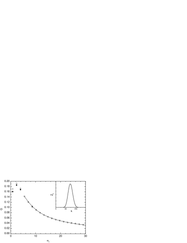
Figure 1: Local Green function of the two-band rotationally invariant model at the Matsubara frequencies. Filled and open circles correspond to the static and to the nonlocal in time spin-flip, respectively. High-frequency asymptotics is drawn with line. Inset shows the distribution function for the perturbation order $k$.

Figure 2: Imaginary-time Green Function (upper panel) and the four-point correlator $\chi$ (lower panel) for two band model. Upper inset shows DOS computed from the Green function. Solid and dot lines correspond to the static and to the nonlocal in time spin-flip, respectively. Lower inset shows DOS for 5 band model with the same value of U and J=0.2

We apply the proposed continuous time QMC for the important problem of super-symmetric two band impurity model at half-filling Rozenberg ; Dworin . To our knowledge, this is the first successful attempt to take the off-diagonal exchange terms of this model into account. These terms are important for the realistic study of multi-band Kondo problem, because they are responsible for the local moment formation Dworin . The interaction in this model has the following form

$$\frac{U}{2}(\hat{N}(\tau)-2)(\hat{N}(\tau)-2)-\frac{J}{2}({\bf S}(\tau)\cdot{\bf S}(\tau)+{\bf L}(\tau)\cdot{\bf L}(\tau)),$$ (8)

where $\hat{N}$ is the operator of total number, $S$ and $L$ are total spin and orbital-momentum operators, respectively. The interaction is spin- and orbital- rotationally invariant. The Gaussian part of the action represents the diagonal semicircular density of states DMFT with unitary half-band width: $t(\omega)=2/(\omega_{n}+\sqrt{\omega_{n}^{2}-1})$, where $\omega_{n}$ are Matsubara frequencies related to imaginary time variable. We used parameters $U=4,J=1$ at $\beta=4$. A modification of this model was also studied, where spin-flip operators were replaced with the fully non-local in time terms. For example, operator $c^{\dagger}_{0\uparrow\tau}c^{0\downarrow\tau}c^{\dagger}_{1\downarrow\tau}c^{1\uparrow\tau}$ was replaced with $\beta^{-1}\int d\tau^{\prime}c^{\dagger}_{0\uparrow\tau}c^{0\downarrow\tau}c^{\dagger}_{1\downarrow\tau^{\prime}}c^{1\uparrow\tau^{\prime}}$. Figures present the result for the local Green function $G_{is}^{is}$ and the four-point correlator $\chi(\tau-\tau^{\prime})=<c^{\dagger}_{0\uparrow\tau}c^{0\downarrow\tau}c^{\dagger}_{1\downarrow\tau^{\prime}}c^{1\uparrow\tau^{\prime}}>$. The later quantity characterizes the spin-spin correlations and would vanish if the exchange is absent.

Figure 1 shows the Green function at Matsubara frequencies. The typical number of QMC trials was $2\cdot 10^{7}$. Results for the local and non-local in time spin-flip are shown with filled and open circles, respectively. The distribution function for the perturbation order $k$ is drawn in the inset. For the system studied it appears to be a Gaussian-like peak located at $k\approx 75$, with an acordance to Eq. (7). The estimated error bar in $G(\omega_{n})$ is about $3\cdot 10^{-3}$ for the lowest frequency and becomes smaller as the frequency increases. The high-frequency tail obeys an asymptotic behavior $-{\rm Im}(iw+\epsilon)^{-1}$ with $\epsilon\approx 2.9$.

Green function in the time domain was obtained by a numerical Fourier-transform from the data for $G(\omega_{n})$. For high harmonics the above-mentioned asymptotic was used. Results are presented in the upper panel of Fig.2. The lower panel presents the result for $\chi(\tau)$. Thess data are obtained similarly, the difference is that $\chi(\omega)$ is defined at Bose Matsubara frequencies and obeys a $1/\omega^{2}$ decay. It is interesting to note that Green function is almost insensitive to the details of spin-flip retardation. Both Green functions are very similar and correspond to qualitatively the same density of states (DOS). The maximum-entropy guess for DOS is presented in the inset to Fig.2. On the other hand, switch to the non-local in time exchange modifies $\chi(\tau)$ dramatically. The local in time exchange results in a pronounces peak of $\chi(\tau)$ at $\tau\approx 0$, whereas the non-local spin-flip results in almost time-independent spin-spin correlations. For realistic description of Kondo impurities like cobalt atom on metallic surface it is of crucial importance to use the spin and orbital rotationally invariant Coulomb vertex in the non-perturbative investigation of electronic structure. The proposed continuous time QMC scheme is easily generalized for a general multiband case. As example we shows the DOS for five d-orbital model at half-filling for the same value of U and J=0.2 in the lower insert of Fig.2.

For a final discussion it is suitable to analyze a convergence of the series (2). Fermi statistics and a finite size of the system insure us that the configurational space of the problem is of a finite order. Because the perturbation operator $W$ has a finite norm, its powers $W^{k}$ therefore grow slower than $k!$. Consequently, from the mathematical point of view there is no doubt that the series (2) always converges. Physically it is important to note that this convergence is related both with a choice of the type of serial expansion and with the peculiarities of the system under study. First of all, series (2) contains all diagrams, including non-bounded. In the analytical diagram-series expansion non-bounded diagrams drop out from the calculation IZ , and the convergence radius for the diagram-series expansion differs from that of (2). Further, Fermi statistics is indeed important. An analog of (2) for Bose field can diverge even for a single-atom problem IZ , because in this case one deals with an infinite-order Gilbert space. It is important to keep this in mind for possible extensions of the algorithm to the electron-phonon systems and to the field models, as these systems are also characterized by an infinite-order phase space. A general time-dependent form of the action (Eq. (1)) allowed us to use renormalization theory for the Hubbard-like model: in this case local DMFT would be a starting point for lattice calculations in order to reduce the effective interaction and minimize the sign problem.

In conclusion, we have developed a fermionic continuous time quantum Monte Carlo method for general non-local in space and time interactions. We demonstrated that for a Hubbard-type models the computational time for a single trial step scales similarly to that for the schemes based on a Stratonovich transformation. An important difference occurs however for the non-local interactions. Consider, for example, a system with a large Hubbard $U$ and much smaller but still important Coulomb interatomic interaction. One needs to introduce $N^{2}$ auxiliary fields per time slice instead of $N$ to take the long-range forces into account. On the other hand, the complexity of the present algorithm should remain almost the same as for the local interactions, because $\overline{|W|}$ does not change much. This should be useful for the realistic cluster DMFT calculations and for the applications to quantum chemistry qchem . It is also possible to study the interactions retarded in time, particularly the super-exchange and the effects related to dissipation. This was demonstrated for an important case of the fully rotationally invariant two band model and its extension with non-local in time spin-flip terms.

We are grateful to A. Georges, M. Katsnelson and F. Assaad for their very valuable comments. This research was supported in part by the National Science Foundation under Grant No. PHY99-07949, ”Russian Scientific Schools” Grant 96-1596476. Authors would like to acknowledge a hospitality of KITP at Santa Barbara University and (AR) University of Nijmegen.

References

- (1) D. J. Scalapino and R.L. Sugar, Phys. Rev. Lett. 46, 519 (1981).
- (2) R. Blankenbecler, D. J. Scalapino, and R. L. Sugar, Phys. Rev. D 24, 2278 (1981).
- (3) J.E. Hirsch, Phys. Rev. B 28, 4059 (1983).
- (4) J. E. Hirsch, Phys. Rev. B 31, 4403 (1985).
- (5) S.R. White J. of Chem. Phys., 117 7472 (2002).
- (6) S.W. Zhang and H. Krakauer, Phys. Rev. Lett. 90, 136401 (2003).
- (7) A. Georges, G. Kotliar, W. Krauth, and M.J. Rozenberg, Rev. Mod. Phys. 68, 13 (1996).
- (8) P. Sun, G. Kotliar Phys. Rev. B 66 085120 (2002).
- (9) M. Capone, M. Fabrizio, C. Castellani, and E. Tosatti Science 296 2364 (2002).
- (10) S. Y. Savrasov, G. Kotliar, and E. Abrahams, Nature 410, 793 (2001).
- (11) A. W. Sandvik and J. Kurkija rvi, Phys. Rev. B 43, 5950 (1991).
- (12) N. V. Prokof ev, B. V. Svistunov, and I. S. Tupitsyn, Pis ma Zh. Eksp. Teor. Fiz. 64, 853 (1996) [JETP Lett. 64, 911 (1996)].
- (13) J. Hubbard, Phys. Rev. Lett 3, 77 (1959), R.L. Stratonovich, Dokl. Akad. Nauk SSSR 115, 1097 (1957).
- (14) M. Jarrell,T. Maier, C. Huscroft, and S. Moukouri Phys. Rev. B 64 195130 (2001).
- (15) B. B. Beard and U.-J. Wiese, Phys. Rev. Lett. 77, 5130 (1996).
- (16) P. E. Kornilovitch, Phys. Rev. Lett. 81, 5382 (1998).
- (17) S. M. A. Rombouts, K. Heyde, and N. Jachowicz, Phys. Rev. Lett. 82, 4155 (1999).
- (18) A.N. Rubtsov, cond-mat/0302228.
- (19) G. G. Batrouni and P. de Forcrand, Phys. Rev. B 48, 589 (1993).
- (20) L. Dworin and A. Narath, Phys. Rev. Lett 1287, 25 (1970).
- (21) M.J. Rozenberg, Phys.Rev. B 55 R4855 (1997)
- (22) C. Itzykson, J.-B. Zuber: Quantum Field Theory. McGraw-Hill (1980)