Ab Initio Studies of Liquid and Amorphous Ge

Abstract

We review our previous work on the dynamic structure factor $S(k,\omega)$ of liquid Ge ($\ell$-Ge) at temperature $T=1250$ K, and of amorphous Ge ($a$-Ge) at $T=300$ K, using ab initio molecular dynamics [Phys. Rev. B67, 104205 (2003)]. The electronic energy is computed using density-functional theory, primarily in the generalized gradient approximation, together with a plane wave representation of the wave functions and ultra-soft pseudopotentials. We use a 64-atom cell with periodic boundary conditions, and calculate averages over runs of up to about 16 ps. The calculated liquid $S(k,\omega)$ agrees qualitatively with that obtained by Hosokawa et al, using inelastic X-ray scattering. In $a$-Ge, we find that the calculated $S(k,\omega)$ is in qualitative agreement with that obtained experimentally by Maley et al. Our results suggest that the ab initio approach is sufficient to allow approximate calculations of $S(k,\omega)$ in both liquid and amorphous materials.

I Introduction

Ge is a well-known semiconductor in its solid phase, but becomes metallic in its liquid phase. Liquid Ge ($\ell$-Ge) has, near its melting point, an electrical conductivity characteristic of a reasonably good metal ($\sim 1.6\times 10^{-4}\Omega^{-1}$cm^-1glazov ), but it retains some residual structural features of the solid semiconductor. For example, the static structure factor $S(k)$, has a shoulder on the high-$k$ side of its first (principal) peak, which is believed to be due to a residual tetrahedral short-range order. This shoulder is absent in more conventional liquid metals such as Na or Al, which have a more close-packed structure in the liquid state and a shoulderless first peak in the structure factor. Similarly, the bond-angle distribution function just above melting is believed to have peaks at two angles, one near $60^{o}$ and characteristic of close packing, and one near $108^{o}$, indicative of tetrahedral short range order. This latter peak rapidly disappears with increasing temperature in the liquid state.

These striking properties of $\ell$-Ge have been studied theoretically by several groups. Their methods fall into two broad classes: empirical and first-principles. A typical empirical calculation is that of Yu et alyu , who calculate the structural properties of $\ell$-Ge assuming that the interatomic potentials in $\ell$-Ge are a sum of two-body and three-body potentials of the form proposed by Stillinger and Webersw . These authors find, in agreement with experiment, that there is a high-k shoulder on the first peak of S(k) just above melting, which fades away with increasing temperature. However, since in this model all the potential energy is described by a sum of two-body and three-body interactions, the interatomic forces are probably stronger, and the ionic diffusion coefficient is correspondingly smaller, than their actual values.

In the second approach, the electronic degrees of freedom are taken explicitly into account. If the electron-ion interaction is sufficiently weak, it can be treated by linear response theoryas . In linear response, the total energy in a given ionic configuration is a term which is independent of the ionic arrangement, plus a sum of two-body ion-ion effective interactions. These interactions typically do not give the bond-angle-dependent forces which are present in the experiments, unless the calculations are carried to third order in the electron-ion pseudopotentialas , or unless electronic fluctuation forces are includednuovo Such interactions are, however, included in the so-called ab initio approach, in which the forces on the ions are calculated from first principles, using the Hellman-Feynman theorem together with density-functional theoryhohenberg ; kohn ; mermin to treat the energy of the inhomogeneous electron gas. This approach not only correctly gives the bond-angle-dependent ion-ion interactions, but also, when combined with standard molecular dynamics techniques, provides a good account of the electronic properties and such dynamical ionic properties as the ionic self-diffusion coefficients.

This combined approach, usually known as ab initio molecular dynamics, was pioneered by Car and Parrinellocar , and, in somewhat different form, has been applied to a wide range of liquid metals and alloys, including $\ell$-Gekresse ; takeuchi ; kulkarni , $\ell$-Ga_xGe_1-xkulkarni1 , stoichiometric III-V materials such as $\ell$-GaAs, $\ell$-GaP, and $\ell$-InPzhang ; lewis , nonstoichiometric $\ell$-Ga_xAs_1-xkulkarni2 , $\ell$-CdTecdte , and $\ell$-ZnTeznte , among other materials which are semiconducting in their solid phases. It has been employed to calculate a wide range of properties of these materials, including the static structure factor, bond-angle distribution function, single-particle electronic density of states, d. c. and a. c. electrical conductivity, and ionic self-diffusion coefficient. The calculations generally agree quite well with available experiment.

A similar ab initio approach has also been applied extensively to a variety of amorphous semiconductors, usually obtained by quenching an equilibrated liquid state from the melt. For example, Car, Parrinello and their collaborators have used their own ab initio approach (based on treating the Fourier components of the electronic wave functions as fictitious classical variables) to obtain many structural and electronic properties of amorphous Sicar1 ; stich . A similar approach has been used by Lee and Changlee . Kresse and Hafnerkresse obtained both S(k) and g(r), as well as many electronic properties, of $a$-Ge, using an ab initio approach similar to that used here, in which the forces are obtained directly from the Hellmann-Feynman theorem and no use is made of fictitious dynamical variables for the electrons, as in the Car-Parrinello approach. A similar calculation for $a$-Si has been carried out by Cooper et alcooper , also making use of a plane wave basis and treating the electron density functional in the generalized gradient approximation (GGA)gga . More recently, a number of calculations for $a$-Si and other amorphous semiconductors have been carried out by Sankey et alsankey , and by Drabold and collaborators drabold . These calculations use ab initio molecular dynamics and electronic density functional theory, but in a localized basis. A recent study, in which S(k) and g(r) were computed for several ab initio structural models of $a$-Si, has been carried out by Alvarez et alalvarez .

Finally, we mention a third approach, intermediate between empirical and ab initio molecular dynamics, and generally known as tight-binding molecular dynamics. In this approach, the electronic part of the total energy is described using a general tight-binding Hamiltonian for the band electrons. The hopping matrix elements depend on separation between the ions, and additional terms are included to account for the various Coulomb energies in a consistent way. The parameters can be fitted to ab initio calculations, and forces on the ions can be derived from the separation-dependence of the hopping matrix elements. This approach has been used, e. g., to treat $\ell$-Siwang1 , $a$-Siservalli , and liquid compound semiconductors such as $\ell$-GaAs and $\ell$-GaSbmolteni . Results are in quite good agreement with experiment.

In this paper, we review the application of ab initio molecular dynamics to another dynamical property of the ions: the dynamical structure factor, denoted $S(k,\omega)$. While no fundamentally new theory is required to calculate $S(k,\omega)$, this quantity provides additional information about the time-dependent ionic response beyond what can be extracted from other quantities Chai . The work we review is the first to calculate $S(k,\omega)$ using ab initio molecular dynamics. Here, we will describe calculations of $S(k,\omega)$ for $\ell$-Ge, where some recent experimentshosokawa provide data for comparison, and also for amorphous Ge ($a$-Ge). In the latter case, using a series of approximations described below, we are able to infer the vibrational density of states of as-quenched $a$-Ge near temperature $T=300$K in reasonable agreement with experiment. The calculated $S(k,\omega)$ for the liquid also agrees quite well with experiment, especially considering the computational uncertainties inherent in an ab initio simulation with its necessarily small number of atoms and limited time intervals.

The remainder of this paper is organized as follows. A brief review of the theory and calculational method is given in Section II and III respectively. The results are reviewed in Section IV, followed by a discussion in Section V.

II Finite-Temperature Density-Functional Theory

The original Hohenberg-Kohn theorem of density-functional theory (DFT) hohenberg was generalized to finite temperatures $T_{el}$ by Mermin mermin . In this section, we give a brief review of the finite-temperature density-functional theory, in a form where it can be used in ab initio molecular dynamics calculations. We use atomic units here and throughout this article.

In the Born-Oppenheimer approximation, the total potential energy U of a system of N classical ions, enclosed in a volume V, and interacting with $N_{el}$=NZ valence electrons through an electron-ion pseudopotential $v_{ei}(r)$, is a functional of the valence electron density $\rho({\bf r})$, and also a function of the ion positions ${\bf R}_{l}$ (l=1,2,…,N). This potential energy can be expressed as the sum of a direct Coulombic interaction between the ions and the free energy $F_{el}$ of the electronic system subject to the external potential created by the ions, which we denote $V_{ext}({\bf r},\{{\bf R}_{l}\})=\sum_{l=1}^{N}v_{ei}(|{\bf r}-{\bf R}_{l}|)$. This sum may be written

$$U[\rho({\bf r}),\{{\bf R}_{l}\}]=F_{el}[\rho({\bf r})]+\sum_{l<l^{\prime}}W({\bf R}_{l}-{\bf R}_{l^{\prime}}),$$ (1)

where $W({\bf R}-{\bf R}^{\prime})=Z^{2}/|{\bf R}-{\bf R}^{\prime}|$ is the Coulomb interaction between ions of charge $Z$ located at ${\bf R}$ and ${\bf R}^{\prime}$.

The free energy functional of the electronic system $F_{el}[\rho({\bf r})]$ can be partitioned into various terms as follows:parr ; dreizler

$$F_{el}[\rho({\bf r})]=A_{s}[\rho({\bf r})]+\int\rho({\bf r})V_{ext}({\bf r})d{\bf r}+\frac{1}{2}\int\frac{\rho({\bf r})\rho({\bf r^{\prime}})}{|{\bf r}-{\bf r^{\prime}}|}d{\bf r}d{\bf r^{\prime}}+F_{xc}[\rho({\bf r})].$$ (2)

Here the different terms are $A_{s}[\rho({\bf r})]$, the Helmholz free energy functional for a reference system of noninteracting electrons; the interaction energy between the valence electrons and the external potential provided by the instantaneous ionic configuration; the classical electron-electron potential energy; and the exchange-correlation correction $F_{xc}[\rho({\bf r})]$ to the free energy. $A_{s}[\rho({\bf r})]$ has contributions from both the kinetic energy $T_{s}[\rho({\bf r})]$ and the entropy $S_{s}[\rho({\bf r})]$ of the reference system, and may be written

$$A_{s}[\rho({\bf r})]=T_{s}[\rho({\bf r})]-T_{el}S_{s}[\rho({\bf r})],$$ (3)

where $T_{el}$ is the temperature of the electronic system.

For a given set of ionic positions, the equilibrium electronic number density $\rho({\bf r})$ is obtained from the following variational principle:

$$\frac{\delta}{\delta\rho({\bf r})}(U[\rho({\bf r}),\{{\bf R}_{l}\}]-\mu\int\rho({\bf r})d{\bf r})=0.$$ (4)

Here $\mu$ is the electron chemical potential, which is chosen to give the desired number of valence electrons $N_{el}$. The Euler equation associated with eq. (4) is

$$\mu=V_{A_{s}}({\bf r};[\rho])+V_{eff}({\bf r};[\rho]).$$ (5)

Here

$$V_{A_{s}}({\bf r};[\rho])=\frac{\delta A_{s}[\rho]}{\delta\rho({\bf r})}$$ (6)

is a functional derivative of $A_{s}[\rho]$, and is the ”Helmholz free energy potential” (or the kinetic potential for $T_{el}=0$) King . $V_{eff}({\bf r};[\rho])$ is an effective one-body potential, given by

$$V_{eff}({\bf r};[\rho])=V_{ext}({\bf r})+\int\frac{\rho({\bf r^{\prime}})}{|{\bf r}-{\bf r^{\prime}}|}d{\bf r^{\prime}}+\frac{\delta F_{xc}[\rho]}{\delta\rho({\bf r})}.$$ (7)

It is usual to make several approximations for the functionals $A_{s}[\rho]$ and $F_{xc}[\rho]$, and the function $V_{ext}({\bf r})$. First, $F_{xc}[\rho]$ is only a minor contribution to $F_{el}[\rho]$. As a result, this functional is often calculated using the local density approximation (LDA) and or the generalized gradient approximation (GGA); both are widely used in many applications parr .

Furthermore, $F_{xc}$ differs negligibly from its zero-temperature value, the exchange-correlation energy $E_{xc}$, provided $T_{el}<0.15T_{f}$, where $T_{f}$ is the Fermi temperature kanhere . Most applications involve temperatures satisfying this inequality. The external field $V_{ext}({\bf r})$ contains the electron-ion pseudopotential $v_{ei}(r)$, on which other approximations are made. For example, it is common to approximate $v_{ei}$ as local and energy-independent.

Once an accurately approximated $A_{s}[\rho]$ is available, one can, in principle, obtain $V_{A_{s}}({\bf r};[\rho])$ by functional differentiation, and from this functional, solve eq. (5) to obtain the equilibrium electronic density. However, this approach has proved to be very challenging in practice.

Typically, the kinetic energy $T_{s}[\rho]$ is much larger than the entropy contribution $T_{el}S_{s}[\rho]$ in the range of temperature interested. Therefore, $A_{s}[\rho]$ is generally well approximated by $T_{s}[\rho]$. However, simple local density approximations for $T_{s}[\rho]$ based on the Thomas-Fermi (TF) theory are not very accurate, and make several qualitatively incorrect predictions thomas ; fermi . More recent developments based on so-called “orbital-free”(OF) approximations for the kinetic energy functional $T_{s}[\rho]$ YWang ; L-WWang ; YWang1 ; YWang2 , and the kinetic potential $V_{T_{s}}({\bf r};[\rho])$ Chai1 ; Chai2 are still insufficient to make quantitative predictions. On the other hand, although these OF methods are currently unable to make accurate predictions, they are computationally appealing, because the computational time required to use them is independent of the number of valence electrons. Therefore, further refinement of such OF methods in DFT may lead to valuable new approaches for investigating the properties of large systems, especially metallic systems.

Instead of using approximate forms for $A_{s}[\rho]$ or $V_{A_{s}}({\bf r};[\rho])$, Kohn and Sham suggested a different way to compute the numerical value of $A_{s}$ exactly, by introducing a set of $N_{el}$ orbitals satisfying the coupled KS equations that describe the model system kohn . Using these orbitals one can determine both $A_{s}$ and the valence electron density $\rho({\bf r})$. The orbitals $\psi_{i}$ satisfy the Schrödinger-like equation

$$\left[-\frac{1}{2}\nabla^{2}+V_{eff}({\bf r})\right]\psi_{i}=\epsilon_{i}\psi_{i},$$ (8)

and are chosen to be orthonormal. The set of equations is made self-consistent by requiring that

$$\rho({\bf r})=\sum_{i}f_{i}|\psi_{i}({\bf r}).|^{2}$$ (9)

Here $f_{i}$ is the Fermi occupation number, given by

$$f_{i}=f(\epsilon_{i}-\mu)=(exp(\frac{\epsilon_{i}-\mu}{k_{B}T_{el}})+1)^{-1}.$$ (10)

The kinetic energy $T_{s}$ is given by

$$T_{s}[\{\psi_{i}({\bf r})\},\{f_{i}\}]=\sum_{i}f_{i}\int\psi_{i}(-\frac{1}{2}\nabla^{2})\psi_{i}d{\bf r}=\sum_{i}\epsilon_{i}f_{i}-\int\rho({\bf r})V_{eff}({\bf r})d{\bf r},$$ (11)

and the electronic entropy $S_{s}$ by

$$S_{s}[\{f_{i}\}]=-2k_{B}\sum_{i}[f_{i}lnf_{i}+(1-f_{i})ln(1-f_{i})]$$ (12)

Eqs.  (7,8,9,10) have to be solved self-consistently. The resulting valence electron density can be used to computed the electronic free energy $F_{el}[\rho]$; the electronic kinetic energy $T_{s}$ and entropy $S_{s}$ are given by eq(11) and eq(12) parr .

The use of finite-temperature DFT is important, in order to eliminate the instability of the KS equations at $T_{el}=0$. In practice, $T_{el}$ is usually regarded as a fictitious temperature (chosen for maintaining the stability), and does not necessarily have to equal the ionic temperature T. Furthermore, the broadening function in eq. (10) need not be the Fermi function, but may be chosen to be some other convenient function. Several possible broadening functions have been proposed kresse ; methfessel .

The forces on the individual ions can now be obtained using the Hellmann-Feynman theorem. According to this theorem, the force ${\bf F}_{I}$ acting on the $I^{th}$ ion is found by differentiating the potential energy of the system with respect to the ionic coordinate ${\bf R}_{I}$weinert ; wentzcovitch . Specifically,

$${\bf F}_{I}=-\frac{\partial U}{\partial{\bf R}_{I}}=-\sum_{i}f_{i}<\psi_{i}|\frac{\partial F_{el}[\rho({\bf r})]}{\partial{\bf R}_{I}}|\psi_{i}>-\frac{\partial}{\partial{\bf R}_{I}}\sum_{l<l^{\prime}}W({\bf R}_{l}-{\bf R}_{l^{\prime}})$$ (13)

Given the force, one simply applies Newton’s second law to get the equations of motion of the $N$ classical ions:

$$M_{I}{\ddot{\bf R}}_{I}={\bf F}_{I}$$ (14)

In practice, the ions are treated classically, even though the origin of the force is very much quantum-mechanical.

In solving these equations of motion, it is important to maintain the ionic temperature T at a fixed value. This is typically accomplished by rescaling the total kinetic energy of the ions $K_{I}$=$\sum_{l=1}^{N}\frac{{\bf P}_{l}^{2}}{2M_{l}}$ to satisfy

$$T=\frac{2K_{I}}{3k_{B}(N-1)}$$ (15)

every few time steps. The factor of N-1, not N, appears here so as to conserve the total momentum of the system of ions.

In summary, for each instantaneous configuration of ions, one computes $F_{el}[\rho({\bf r})]$ and hence $U[\rho({\bf r}),\{{\bf R}_{l}\}]$ by solving the finite-temperature Kohn-Sham equations (7),(8),(9), and (10). The Hellmann-Feynman force ${\bf F}_{I}$ is then computed from eq. (13). By numerically solving Newton’s equations of motion for the ions and rescaling the kinetic energy of the ions at every time step, one moves the ions to a new configuration. The entire process is repeated for a sufficiently large number of time steps to compute the desired property with good statistical accuracy.

III METHOD

The method we have used to calculate the dynamic structure factorChai is similar to that described in several previous papers for other properties of liquid semiconductorskulkarni ; kulkarni1 ; kulkarni2 , but uses the Vienna Ab Initio Simulation Package (VASP), whose workings have been extensively described in the literaturekresse1 .” Briefly, the calculation involves two parts. First, for a given ionic configuration, the total electronic energy is calculated, using an approximate form of the Kohn-Sham free energy density functional, and the force on each ion is also calculated, using the Hellmann-Feynman theorem. Second, Newton’s equations of motion are integrated numerically for the ions, using a suitable time step. The process is repeated for as many time steps as are needed to calculate the desired quantity. To hold the temperature constant, we use the canonical ensemble with the velocity rescaled at each time step. Further details of this approach are given in Ref. kulkarni .

The VASP code uses the ultrasoft Vanderbilt pseudopotentialsvanderbilt , a plane wave basis for the wave functions, with the original Monkhorst-Pack ($3\times 3\times 3$) k-space meshesmonkhorst and a total of 21,952 plane waves, corresponding to an energy cut-off of 104.4eV. We have used a finite-temperature version of the Kohn-Sham theorymermin in which the electron gas Helmholtz free energy is calculated on each time step. This version also broadens the one-electron energy levels to make the k-space sums converge more rapidly. The method of Methfessel-Paxton of order 1 is used for the broadening function methfessel ., with the fictitious temperature for the electronic subsystem $k_{B}T_{el}$=0.2 eV. Most of our calculations were done using the generalized gradient approximation (GGA)gga for the exchange-correlation energy (we use the particular form of the GGA developed by Perdew and Wanggga ), but some are also carried out using the local-density approximation (LDA).

In our iteration of Newton’s Laws in liquid Ge ($\ell$-Ge), we typically started from the diamond structure (at the experimental liquid state density for the temperature of interest), then iterated for 901 time steps, each of 10 fs, using the LDA. To obtain S(k) within the GGA, we started from the LDA configuration after 601 time steps, then iterated using the GGA for an additional 1641 10-fs time steps, or 16.41 ps. We calculate the GGA S(k) by averaging over an interval of 13.41 ps within this 16.41 time interval, starting a time $t_{2}$ after the start of the GGA simulation. We average over all $t_{2}$’s from 1.0 to 3.0 ps.

For comparison, we have also calculated S(k) within the LDA. This S(k) is obtained by averaging over 601 time steps of the 901 time-step LDA simulation. This 601-step interval is chosen to start a time $t_{1}$ after the start of this simulation; the calculated LDA S(k) is also averaged over all $t_{1}$’s from 1.0 ps to 3.0 ps.

To calculate quantities for amorphous Ge (a-Ge), we start with Ge in the diamond structure at T = 1600K but at the calculated liquid density for that temperature, as given in Ref. kulkarni . Next, we quench this sample to 300 K, cooling at a uniform rate over, so as to reach 300 K in about 3.25 ps (in 10-fs time steps). Finally, starting from T = 300 K, we iterate for a further 897 time steps, each of 10 fs, or 8.97 ps, using the LDA. The LDA S(k) is then obtained by averaging over 5.97 of those 8.97 ps, starting a time $t_{1}$ after the system is reached 300K; we also average this S(k) over all $t_{1}$’s from 1.0 to 3.0 ps. To obtain S(k) within the GGA, we start the GGA after 5.7 ps of the LDA simulation, and then iterate using the GGA for an additional 18.11 ps in 10-fs time steps. The GGA S(k) is obtained by averaging over a 15.11 ps time interval of this 18.11 ps run, starting a time $t_{2}$ after the start of the GGA simulation; we also average over all values of $t_{2}$ from 1.0 to 3.0 ps.

The reader may be concerned that the 3.25 ps quench time is very short, very unrepresentative of a realistic quench, and very likely to produce numerous defects in the quenched structure, which are not typical of the $a$-Ge studied in experiments. In defense, we note that some of these defects may be annealed out in the subsequent relaxation at low temperatures, which is carried out before the averages are taken. In addition, the static structure factor we obtain agrees well with experiment, and the dynamic structure factor is also consistent with experiment, as discussed below. Thus, the quench procedure appears to produce a material rather similar to some of those studied experimentally. Finally, we note that experiments on $a$-Ge themselves show some variation, depending on the exact method of sample preparation.

We have used the procedure outlined above to calculate various properties of $\ell$-Ge and $a$-Ge. Most of these calculated properties have been described in previous papers, using slightly different methods, and therefore will be discussed here only very brieflycompare . However, our results for the dynamic structure factor $S(k,\omega)$ as a function of wave vector k and frequency $\omega$ are new, and will be described in detail. We also present our calculated static structure factor $S(k)$, which is needed in order to understand the dynamical results.

$S(k)$ is defined by the relation

$$S(k)=\frac{1}{N}\langle\sum_{i,j}\exp[i{\bf k}\cdot({\bf r}_{i}(t)-{\bf r}_{j}(t))]\rangle_{t_{0}}-N\delta_{{\bf k},0},$$ (16)

where ${\bf r}_{i}$ is the position of the i^th ion at time t, $N$ is the number of ions in the sample, and the triangular brackets denote an average over the sampling time. In all our calculations, we have used a cubic cell with $N=64$ and periodic boundary conditions in all three directions. This choice of particle number and cell shape is compatible with any possible diamond-structure Ge within the computational cell.

$S({\bf k},\omega)$ is defined by the relation (for ${\bf k}\neq 0$, $\omega\neq 0$)

$$S({\bf k},\omega)=\frac{1}{2\pi N}\int_{-\infty}^{\infty}\exp(i\omega t)\langle\rho({\bf k},t)\rho(-{\bf k},0)\rangle dt,$$ (17)

where the Fourier component $\rho({\bf k},t)$ of the number density is defined by

$$\rho({\bf k},t)=\sum_{i=1}^{N}\exp(-i{\bf k}\cdot{\bf r}_{i}(t)).$$ (18)

In our calculations, the average $\langle...\rangle$ is computed as

$$\langle\rho({\bf k},t)\rho({\bf-k},0)\rangle=\frac{1}{\Delta t_{1}}\int_{0}^{\Delta t_{1}}\rho({\bf k},t_{1}+t)\rho({\bf-k},t_{1})dt_{1}$$ (19)

over a suitable range of initial times $t_{1}$. Because of the expected isotropy of the liquid or amorphous phase, which should hold in the limit of large N, $S({\bf k},\omega)$ should be a function only of the magnitude $k$ rather than the vector ${\bf k}$, as should the structure factor $S({\bf k})$.

Our calculations are carried out over relatively short times. To reduce statistical errors, we therefore first calculate

$$S({\bf k},\omega,t_{1},t_{2})=\frac{1}{\pi N}\int_{0}^{t_{2}}dt\rho({\bf k},t_{1}+t)\rho(-{\bf k},t_{1})\exp(i\omega t).$$ (20)

For large enough $t_{2}$, $S({\bf k},\omega,t_{1},t_{2})$ should become independent of $t_{2}$ but will still retain some dependence on $t_{1}$. Therefore, in the liquid, we obtain our calculated dynamic structure factor, $S_{calc}({\bf k},\omega)$, by averaging over a suitable range of $t_{1}$ from 0 to $\Delta t_{1}$:

$$S_{calc}({\bf k},\omega)=\frac{1}{\Delta t_{1}}\int_{0}^{\Delta t_{1}}dt_{1}S({\bf k},\omega,t_{1},t_{2}).$$ (21)

We choose our initial time in the $t_{1}$ integral to be 1 ps after the start of the GGA calculation, and (in the liquid) $\Delta t_{1}=6$ ps. We choose the final MD time $t_{2}=16.41$ps. For $a$-Ge, we use the same procedure but $t_{2}=18.11$ps in our simulations. For our finite simulational sample, the calculated $S({\bf k})$ and $S({\bf k},\omega)$ will, in fact, depend on the direction as well as the magnitude of ${\bf k}$. To suppress this finite-size effect, we average the calculated $S({\bf k})$ and $S({\bf k},\omega)$ over all ${\bf k}$ values of the same length. This averaging considerably reduces statistical error in both $S(k,\omega)$ and $S(k)$.

Finally, we have also incorporated the experimental resolution functions into our plotted values of $S(k,\omega)$. Specifically, we generally plot $S_{av}(k,\omega)/S(k)$, where $S_{av}(k,\omega)$ is obtained from the (already orientationally averaged) $S(k,\omega)$ using the formula

$$S_{av}(k,\omega)=\int_{-\infty}^{\infty}R(\omega-\omega^{\prime})S(k,\omega^{\prime})d\omega^{\prime},$$ (22)

where the resolution function $R(\omega)$ (normalized so that $\int_{-\infty}^{\infty}R(\omega)d\omega=1$) is

$$R(\omega)=\frac{1}{\sqrt{\pi}\omega_{0}}\exp(-\omega^{2}/\omega_{0}^{2}).$$ (23)

In an isotropic liquid, we must have $S(k,-\omega)=S(k,\omega)$, since our ions are assumed to move classically under the calculated first-principles force. Our orientational averaging procedure guarantees that this will be satisfied identically in our calculations, since for every ${\bf k}$, we always include ${\bf-k}$ in the same average. We will nonetheless show results for negative $\omega$ for clarity, but they do not provide any additional information.

IV RESULTS

IV.1 S(k) for $\ell$-Ge and $a$-Ge

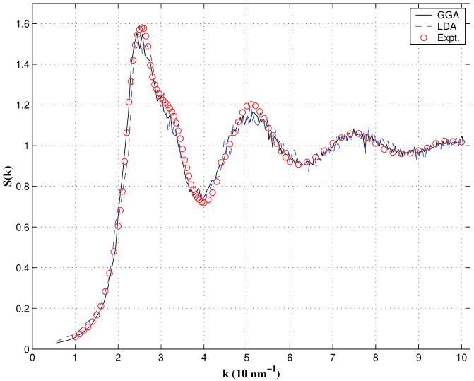
Figure 1: Static structure factor S(k) for $\ell$-Ge at $T=1250K$, just above the experimental melting temperature. Full curve: present work, as calculated using the generalized gradient approximation (GGA; see text). Dashed curve: present work, but using the local density approximation (LDA; see text). Open circles: measured S(k) near $T=1250$ K, as given in Ref. waseda .

In Fig. 1, we show the calculated $S(k)$ for $\ell$-Ge at $T=1250$ K, as obtained using the procedure described in Section II. The two calculated curves are obtained using the GGA and the LDA for the electronic energy-density functional; they lead to nearly identical results. The calculated $S(k)$ shows the well-known characteristics already found in previous simulationskresse ; kulkarni . Most notably, there is a shoulder on the high-$k$ side of the principal peak, which is believed to arise from residual short-range tetrahedral order persisting into the liquid phase just above melting. We also show the experimental results of Waseda et alwaseda ; agreement between simulation and experiment is good, and in particular the shoulder seen in experiment is also present in both calculated curves (as observed also in previous simulations).

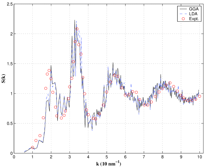
Figure 2: Full curve: Calculated S(k) for $a$-Ge at $T=300K$, as obtained using the GGA. Structure is prepared as described in the text. Open circles: measured S(k) for $a$-Ge at $T=300K$, as given in Ref. etherington .

We have also calculated S(k) for a model of amorphous Ge ($a$-Ge) at $300K$. We prepared our sample of $a$-Ge as described in the previous section. As for $\ell$-Ge, we average the calculated S(k) over different ${\bf k}$ vectors of the same length, as for $\ell$-Ge. In Fig. 2, we show the calculated $S(k)$ for $a$-Ge at T = 300, again using both the GGA and the LDA. The sample is prepared and the averages obtained as described in Section II. In contrast to $\ell$-Ge, but consistent with previous simulationskresse ; alvarez , the principal peak in S(k) is strikingly split. The calculations are in excellent agreement with experiments carried out on as-quenched $a$-Ge at $T=300$ Ketherington ; in particular, the split principal peak seen in experiment is accurately reproduced by the simulations.

We have also calculated a number of other quantities for both $\ell$-Ge and $a$-Ge, including pair distribution function $g(r)$, and the electronic density of states $n(E)$. For $\ell$-Ge, we calculated $n(E)$ using the Monkhorst-Pack mesh with gamma point shifting (one of the meshes recommended in the VASP package). The resulting $n(E)$ is generally similar to that found in previous calculationskresse ; kulkarni , provided that an average is taken over at least 5-10 liquid state configurations. Our $n(E)$ for $a$-Ge [calculated using a shorter averaging time than that used below for $S(k,\omega)$] is also similar to that found previouslykresse . Our calculated $g(r)$’s for both $\ell$-Ge and $a$-Ge, as given by the VASP program, are similar to those found in Refs. kresse and kulkarni . The calculated number of nearest neighbors in the first shell is 4.18 for $a$-Ge measured to the first minimum after the principal peak in g(r). For $\ell$-Ge, if we count as “nearest neighbors” all those atoms within 3.4Åof the central atom (the larger of the cutoffs used in Ref. kresse ) we find approximately 7.2 nearest neighbors, quite close to the value of 6.9 obtained in Ref. kresse for that cutoff. Finally, we have recalculated the self-diffusion coefficient $D(T)$ for $\ell$-Ge at $T=1250$ K, from the time derivative of the calculated mean-square ionic displacement; we obtain a result very close to that of Ref. kulkarni .

IV.2 $S(k,\omega)$ for $\ell$-Ge and $a$-Ge

IV.2.1 $\ell$-Ge

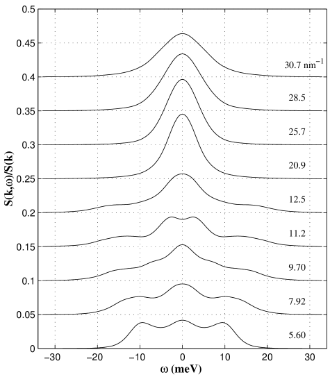
Figure 3: Calculated ratio of dynamic structure factor $S(k,\omega)$ to static structure factor $S(k)$ for $\ell$-Ge at $T=1250K$ for several values of $k$, plotted as a function of $\omega$, calculated using ab initio molecular dynamics with a MD time step of 10 fs. For clarity, each curve has been vertically displaced by 0.05 units from the curve below. In each case, the plotted curve is obtained by averaging both the calculated $S({\bf k},\omega)$ and the calculated $S({\bf k})$ over all values of ${\bf k}$ of the same length. We also incorporate a Gaussian resolution function of half-width $\hbar\omega_{0}=2.5$ meV, as in eqs. (22) and (23). This value of $\omega_{0}$ is chosen to equal the quoted experimental resolutionhosokawa .

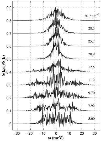
Figure 4: Same as in Fig. 3, but without the resolution function.

Fig. 3 shows the calculated ratio $S(k,\omega)/S(k)$ for $\ell$-Ge at $T=1250$ K, as obtained using the averaging procedure described in Section II. We include a resolution function [eqs. (22) and (23)] of width $\hbar\omega=2.5$ meV, the same as the quoted experimental widthhosokawa . In Fig. 4, we show the same ratio, but without the resolution function (i. e., with $\omega_{0}=0$). Obviously, there is much more statistical noise in this latter case, though the overall features can still be distinguished.

To interpret these results, we first compare the calculated $S(k,\omega)$ in $\ell$-Ge with hydrodynamic predictions, which should be appropriate at small $k$ and $\omega$. The This prediction takes the form (see, for example, Ref. hansen ):

$$2\pi\frac{S(k,\omega)}{S(k)} = \frac{\gamma-1}{\gamma}\left(\frac{2D_{T}k^{2}}{\omega^{2}+(D_{T}k^{2})^{2}}\right)+$$ (24)

$$+ \frac{1}{\gamma}\left(\frac{\Gamma k^{2}}{(\omega+c_{s}k)^{2}+(\Gamma k^{2})^{2}}+\frac{\Gamma k^{2}}{(\omega-c_{s}k)^{2}+(\Gamma k^{2})^{2}}\right).$$

Here $\gamma=c_{P}/c_{V}$ is the ratio of specific heats and constant pressure and constant volume, $D_{T}$ is the thermal diffusivity, $c_{s}$ is the adiabatic sound velocity, and $\Gamma$ is the sound attenuation constant. $D_{T}$ and $\Gamma$ can in turn be expressed in terms of other quantities. For example, $D_{T}=\kappa_{T}/(\rho c_{P})$, where $\kappa_{T}$ is the thermal conductivity and $\rho$ is the atomic number density. Similarly, $\Gamma=\frac{1}{2}\left[a(\gamma-1)/\gamma+b\right]$, where $a=\kappa_{T}/(\rho c_{V})$ and $b$ is the kinematic longitudinal viscosity (see, for example, Ref. hansen , pp. 264-66).

Eq. (24) indicates that $S(k,\omega)$ in the hydrodynamic regime should have two propagating peaks centered at $\omega=\pm c_{s}k$, and a diffusive peak centered at $\omega=0$ and of width determined by $D_{T}$. The calculated $S(k,\omega)/S(k)$ for the three smallest values of $k$ in Fig. 3, does show the propagating peaks. We estimate peak values of $\hbar\omega\sim 10$ meV for $k=5.60$ nm^-1, $\hbar\omega\sim 11$ meV for $k=7.92$ nm^-1, and (somewhat less clearly) $\hbar\omega\sim 13$ meV for $k=9.70$ nm^-1. The value of $c_{s}$ estimated from the lowest $k$ value is $c_{s}\sim 2.7\times 10^{5}$ cm/sec. (The largest of these three $k$ values may already be outside the hydrodynamic, linear-dispersion regime.)

These predictions agree reasonably well with the measured $S(k,\omega)$ obtained by Hosokawa et alhosokawa , using inelastic X-ray scattering. For example, the measured sound-wave peaks for $k=\pm 6$ nm^-1 occur near $10$ meV, while those $k=\pm 12$ nm^-1 occur at $\hbar\omega=17.2$ meV, Furthermore, the integrated relative strength of our calculated sound-wave peaks, compared to that of the central diffusion peak, decreases between $k=7.92$ nm^-1 and $12.5$ nm^-1, consistent with both eq. (24) and the change in experimental behaviorhosokawa between $k=6$ nm^-1 and $12$ nm^-1.

Because $S(k,\omega)$ in Fig. 3 already includes a significant Gaussian smoothing function, a quantitatively accurate half-width for the central peak, and hence a reliable predicted value for $D_{T}$, cannot be extracted. A rough estimate can be made as follows. For the smallest k value of 5.6 nm^-1, the full width of the central peak at half-maximum is around $7.5$ meV. If the only broadening were due to this Gaussian smoothing, the full width would be around $2\hbar\omega_{0}=5.5$ meV. Thus, a rough estimate of the intrinsic full width is $\approx\sqrt{7.5^{2}-5.5^{2}}=5$ meV $\approx 2\hbar D_{T}k^{2}$. This estimate seems reasonable from the raw data for $S(k,\omega)$ shown in Fig. 4. Using this estimate, one obtains $D_{T}\approx 1.3\times 10^{-3}$ cm²/sec.

The hydrodynamic expression for $S(k,\omega)/S(k)$ was originally obtained without consideration of the electronic degrees of freedom. Since $\ell$-Ge is a reasonably good metal, one might ask if the various coefficients appearing eq. (24) should be the full coefficients, or just the ionic contribution to those coefficients. For example, should the value of $D_{T}$ which determines the central peak width be obtained from the full $c_{P}$, $c_{V}$, and $\kappa_{T}$, or from only the ionic contributions to these quantities? For $\ell$-Ge, the question is most relevant for $\kappa_{T}$, since the dominant contribution to $c_{P}$ and $c_{V}$ should be the ionic parts, even in a liquid metalas . However, the principal contribution to $\kappa_{T}$ is expected to be the electronic contribution.

We have made an order-of-magnitude estimate of $D_{T}$ using the experimental liquid number density and the value $C_{P}=(5/3)k_{B}$ per ion, and obtaining the electronic contribution to $\kappa_{T}$ from the Wiedemann-Franz lawam76 together with previously calculated estimates of the electronic contributionkulkarni . This procedure yields $D_{T}\sim 0.1$ cm²/sec, about two orders of magnitude greater than that extracted from Fig. 3, and well outside the possible errors in that estimate. We conclude that the $D_{T}$ which should be used in eq. (24) for $\ell$-Ge (and by inference other liquid metals) is the ionic contribution only.

In support of this interpretation, we consider what one expects for $S(k,\omega)$ in a simple metal such as Na. In such a metal, ionic motions are quite accurately determined by effective pairwise screened ion-ion interactionsas . Since the ionic motion is determined by such an interaction, the $S(k,\omega)$ resulting from that motion should not involve the contribution of the electron gas to the thermal conductivity. Although $\ell$-Ge is not a simple metal, it seems plausible that its $S(k,\omega)$ should be governed by similar effects, at least in the hydrodynamic regime. This plausibility argument is supported by our numerical results.

For $k$ beyond around $12$ nm^-1, the hydrodynamic model should start to break down, since the dimensionless parameter $\omega\tau$ (where $\tau$ is the Maxwell viscoelastic relaxation time) becomes comparable to unity. At these larger $k$’s, both our calculated and the measuredhosokawa curves of $S(k,\omega)/S(k)$ continue to exhibit similarities. Most notable is the existence of a single, rather narrow peak for $k$ near the principal peak of $S(k)$, followed by a reduction in height and broadening of this central peak as $k$ is further increased. This narrowing was first predicted by de Gennesdegennes . In our calculations, it shows up in the plot for $k=20.9$ nm^-1, for which the half width of $S(k,\omega)/S(k)$ is quite narrow, while at $k=28.5$ and $30.7$ nm^-1, the corresponding plots are somewhat broader and lower. By comparison, the measured central peak in $S(k,\omega)/S(k)$ is narrow at $k=20$ nm^-1 and especially at $k=24$ nm^-1, while it is broader and lower at $k=28$ nm^-1hosokawa .

The likely physics behind the de Gennes narrowing is straightforward. The half-width of $S(k,\omega)$ is inversely proportional to the lifetime of a density fluctuation of wave number $k$. If that $k$ coincides with the principal peak in the structure factor, a density fluctuation will be in phase with the natural wavelength of the liquid structure, and should decay slowly, in comparison to density fluctuations at other wavelengths. This is indeed the behavior observed both in our simulations and in experiment.

In further support of this picture, we may attempt to describe these fluctuations by a very oversimplified Langevin model. We suppose that the Fourier component $\rho({\bf k},t)$ [eq. (18)] is governed by a Langevin equation

$$\dot{\rho}({\bf k},t)=-\xi\rho({\bf k},t)+\eta(t).$$ (25)

Here the dot is a time derivative, $\xi$ is a constant, and $\eta(t)$ is a random time-dependent “force” which has ensemble average $\langle\eta\rangle=0$ and correlation function $\langle\eta(t)\eta^{*}(t^{\prime})\rangle=A\delta(t-t^{\prime})$. Eq. (25) can be solved by standard methods (see, e. g., Ref. hansen for a related example), with the result (for sufficiently large t)

$$\langle\rho({\bf k},t)\rho^{*}({\bf k},t+\tau)\rangle=\frac{\pi A}{\xi}\exp(-|\tau|\xi).$$ (26)

According to eq. (17), $S(k,\omega)$ is, to within a constant factor, the frequency Fourier transform of this expression, i. e.

$$S(k,\omega)\propto\int_{-\infty}^{\infty}(\pi A/\xi)\exp(i\omega\tau)\exp(-|\tau|\xi)d\tau,$$ (27)

or, on carrying out the integral,

$$S(k,\omega)\propto\frac{\pi A}{\omega^{2}+\xi^{2}}.$$ (28)

This is a Gaussian function centered at $\omega=0$ and of half-width $\xi$. On the other hand, the static structure factor

$$S(k)\propto Lim_{\tau\rightarrow 0}\langle\rho({\bf k},t)\rho^{*}({\bf k},t+\tau)\rangle=\frac{\pi A}{\xi}.$$ (29)

Thus, if the constant $A$ is independent of ${\bf k}$, the half-width $\xi$ of the function $S(k,\omega)$ at wave number ${\bf k}$ is inversely proportional to the static structure $S(k)$. This prediction is consistent with the “de Gennes narrowing” seen in our simulations and in experimenthosokawa .

To summarize, there is overall a striking similarity in the shapes of the experimental and calculated curves for $S(k,\omega)/S(k)$ both in the hydrodynamic regime and at larger values of $k$.

IV.2.2 $a$-Ge

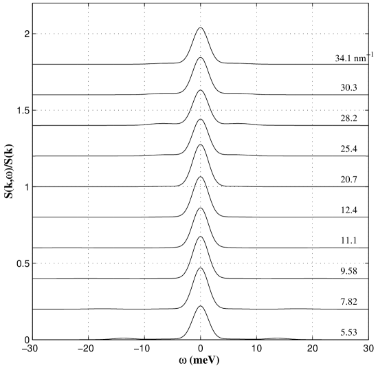
Figure 5: Calculated $S(k,\omega)/S(k)$ for $a$-Ge at $T=300$ K at $k\leq 35$ nn^-1, plotted as a function of $\omega$ Again, each curve has been vertically displaced by appropriate amounts from the one below it, as evident from the Figure, and both $S(k,\omega)$ and $S(k)$ have been plotted after an average over all ${\bf k}$’s of the same length. We also incorporate a Gaussian resolution function of half-width $\hbar\omega_{0}=2$ meV. This value is chosen to give the best results for $n_{vib}(\omega)$ as measured by Ref. maley . The time step here is 10 fs.

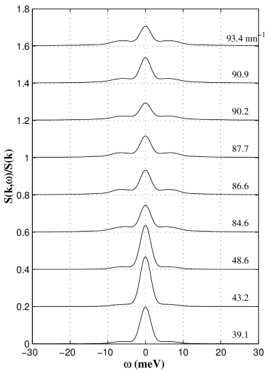
Figure 6: Same as Fig. 5, but at $k\geq 35$ nm^-1.

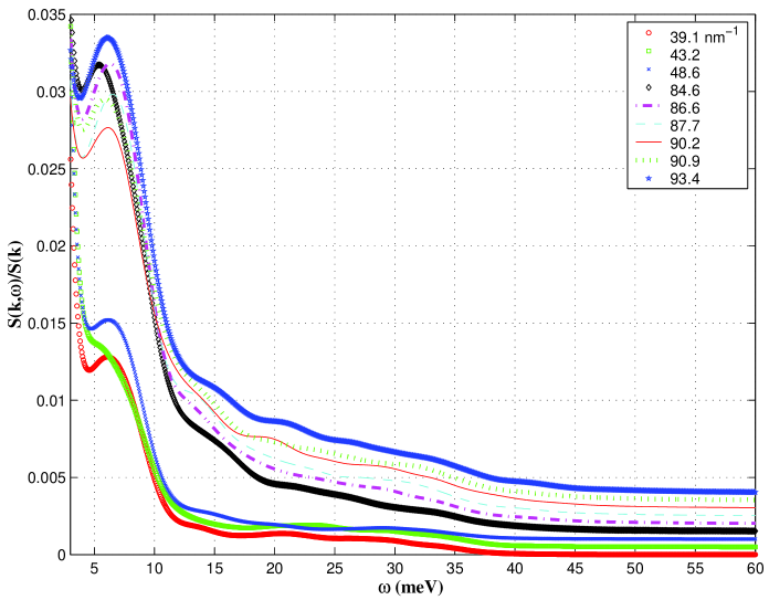
Figure 7: Calculated $S(k,\omega)/S(k)$ as in Figs. 5 and 6 but including higher frequencies $\omega$. At $\hbar\omega=60$ meV, the curves are arranged vertically in order of increasing frequency. Each curve is vertically displaced by 0.0005 units from the one below it.

We have also calculated the dynamic structure for our sample of $a$-Ge at $T=300K$. The results for the ratio $S(k,\omega)/S(k)$ are shown in Figs. 5 and 6 for a range of $k$ values, and, over a broader range of $\omega$, in Fig. 7. Once again, both $S(k,\omega)$ and $S(k)$ are averaged over different values of ${\bf k}$ of the same length, as described above. We have incorporated a resolution function of width $\hbar\omega_{0}=2$ meV into $S(k,\omega)$. This width is a rough estimate for the experimental resolution function in the measurements of Maley et almaley ; we assume it to be smaller than the liquid case because the measured width of the central peak in $S(k,\omega)/S(k)$ for $a$-Ge is quite small.

Ideally, our calculated $S(k,\omega)$ should be compared to the measured one. However, the published measured quantity is not $S(k,\omega)$ but is, instead, based on a modified dynamical structure factor, denoted $G(k,\omega)$, and related to $S(k,\omega)$ bymaley

$$G(k,\omega)=\left(\frac{C}{k^{2}}\right)\left(\frac{\hbar\omega}{n(\omega,T)+1}\right)S(k,\omega).$$ (30)

Here $C$ is a k- and $\omega$-independent constant, and $n(\omega,T)=1/[e^{\hbar\omega/k_{B}T}-1]$ is the phonon occupation number for phonons of energy $E=\hbar\omega$ at temperature $T$. The quantity plotted by Maley et almaley is an average of $G(k,\omega)$ over a range of k values from 40 to 70 nm^-1. These workers assume that this average is proportional to the vibrational density of states $n_{vib}(\omega)$. The measured $n_{vib}(\omega)$ as obtained in this waymaley is shown in Fig. 8 for two different amorphous structures, corresponding to two different methods of preparation and having differing degrees of disorder.

In order to compare our calculated $S(k,\omega)$ to experiment, we use eq. (30) to infer $G(k,\omega)$, then average over a suitable range of k. However, in using eq. (30), we use the classical form of the occupation factor, $n(\hbar\omega)+1\approx k_{B}T/\hbar\omega$, This choice is justified because we have calculated $S(k,\omega)$ using classical equations of motion for the ions. We thus obtain for the calculated vibrational density of states

$$n_{vib}(\omega)\approx\left(\frac{C\hbar^{2}}{k_{B}T}\right)\left(\frac{\omega^{2}}{k^{2}}\right)S(k,\omega).$$ (31)

In Fig. 8 we show two such calculated plots of $n_{vib}(\omega)$, as obtained by averaging eq. (31) over two separate groups of $k$’s, as indicated in the captionnote . For comparison, we also show $n_{vib}(\omega)$ for $a$-Ge as calculated in Ref. kresse directly from the Fourier transform of the velocity-velocity autocorrelation function.

The calculated plots for $n_{vib}(\omega)$ in Fig. 8 have some distinct structure, which arises from some corresponding high frequency structure in $S(k,\omega)$. The plot of $n_{vib}(\omega)$ for the group of smaller k’s has two distinct peaks, near $8$ meV and $29$ meV, separated by a broad dip with a minimum near 18 meV. The plot corresponding to the group of larger k’s has similar structure and width, but the dip is less pronounced. The two experimental plots also have two peaks separated by a clear dip. The two maxima are found around $10$ and $35$ meV, while the principal dip occurs near $16$ meV. In addition, the overall width of the two densities of states is quite similar.

The reasonable agreement between the calculated and measured $n_{vib}(\omega)$ suggests that our ab initio calculation of $S(k,\omega)$ for $a$-Ge is reasonably accurate. The noticeable differences probably arise from several factors. First, there are several approximations involved in going from the calculated and measured $S(k,\omega)$’s to the corresponding $n_{vib}(\omega)$’s, and these may be responsible for some of the discrepancies. Secondly, there may actually be differences between the particular amorphous structures studied in the experiments, and the quenched, then relaxed structure considered in the present calculations. (However, the similarities in the static structure factors suggest that these differences are not vast.) Finally, our calculations are carried out over relatively short times, using relatively few atoms; thus, finite-size and finite-time effects are likely to produce some additional errors. Considering all these factors, agreement between calculation and experiment is quite reasonable.

Previous ab initio calculations for $a$-Gekresse have also obtained a vibrational density of states, but this is computed directly from the ionic velocity-velocity autocorrelation function rather than from the procedure described here. The calculations in Ref. kresse do not require computing $S(k,\omega)$. In the present work, by contrast, we start from our calculated $S(k,\omega)$, and we work backwards to get $n_{vib}(\omega)$. In principle, our $S(k,\omega)$ includes all anharmonic effects on the vibrational spectrum of $a$-Ge, though in extracting $n_{vib}(\omega)$ we assume that the lattice vibrates harmonically about the metastable atomic positions. In Fig. 8, we also show the results of Ref. kresse for $n_{vib}(\omega)$ as obtained from this correlation function. They are quite similar to those obtained in the present work, but have a somewhat deeper minimum between the two principal peaks.

The quantity $n_{vib}(\omega)$ could, of course, also be calculated directly from the force constant matrix, obtained by assuming that the quenched configuration is a local energy minimum and calculating the potential energy for small positional deviations from that minimum using ab initio molecular dynamics. This procedure has been followed for $a$-GeSe₂, for example, by Cappelletti et alcappelletti . These workers have then obtained $S(q,\omega)$ versus $q$ from their $n_{vib}(\omega)$ at selected values of $\omega$, within a one-phonon approximation. However, as noted above, the present work produces the full $S(k,\omega)$ and thus has, in principle, more information than $n_{vib}(\omega)$.

V DISCUSSION AND CONCLUSIONS

The results reviewed here show that ab initio molecular dynamics can be used to calculate the dynamic structure factor $S(k,\omega)$ for both liquid and amorphous semiconductors. Although the accuracy of the calculated $S(k,\omega)$ is lower than that attained for static quantities, such as $S(k)$, nonetheless it is sufficient for comparison to most experimental features. This is true even though our calculations are limited to 64-atom samples and fewer than 20 ps of elapsed real time.

We have presented evidence that the calculated $S(k,\omega)/S(k)$ in $\ell$-Ge agrees qualitatively with measured by inelastic X-ray scatteringhosokawa , and that the one calculated for $a$-Ge leads to a vibrational density of states qualitatively similar to the quoted experimental onemaley . Since such calculations are thus shown to be feasible, the work reviewed here should spur further numerical studies, with longer runs on larger samples, to obtain even more detailed information. Furthermore, we can use these dynamical simulations to probe the underlying processes at the atomic scale which give rise to specific features in the measured and calculated $S(k,\omega)$.

VI ACKNOWLEDGEMENTS

This work has been supported by NSF grants DMR01-04987 (D.S.), DMR04-12295 (D.S.) and CHE01-11104 (J.D.C.). Calculations were carried out using the Beowulf Cluster at the Ohio Supercomputer Center, with the help of a grant of time. Jeng-Da Chai acknowledges full support from the UMCP Graduate School Fellowship, the IPST Alexander Family Fellowship, and the CHPH Block Grant Supplemental Fellowship.

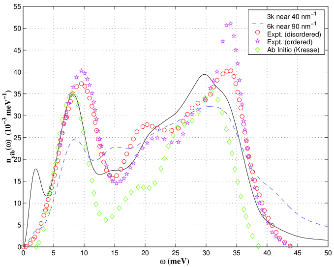
Figure 8: Full curve: calculated vibrational density of states $n_{vib}(\omega)$, in units of $10^{-3}$ states/meV. $n_{vib}(\omega)$ is obtained from the resolution-broadened $S(k,\omega)$ and $S(k)$ of the previous Figure, using the formula $n_{vib}(\omega)=\langle G_{calc}(k,\omega)\rangle$, where $G_{calc}(k,\omega)$ is given by eq. (16), and the averaging is carried out over the three magnitudes of $k$ near $40$ nm^-1 for which we have computed $S(k,\omega)$. Dashed curve: same as full curve, but calculated by averaging over the six magnitudes of $k$ near $90$ nm^-1 for which we have computed $S(k,\omega)$. The open circles and open stars denote the measured $n_{vib}(\omega)$, as reported in Ref. maley for two forms of $a$-Ge. Finally, the open diamonds denote $n_{vib}(\omega)$ as calculated in Ref. kresse from the ionic velocity-velocity autocorrelation function (dot-dashed curves). In all plots except that of Ref. kresse , $n_{vib}(\omega)$ is normalized so that $\int_{0}^{\omega_{max}}n(\omega)d(\hbar\omega)=1$. $\omega_{max}$ is the frequency at which $n_{vib}(\omega)\rightarrow 0$, and is estimated from this Figure by extrapolating the right hand parts of the solid and dashed curves linearly to zero.

References

- (1) V. M. Glazov, S. N. Chizhevskaya, and N. N. Glagoleva, Liquid Semiconductors (Plenum, New York, 1969).
- (2) W. B. Yu, Z. Q. Wang, and D. Stroud, Phys. Rev. B54, 13946 (1996).
- (3) F. H. Stillinger and Weber, Phys. Rev. B31, 5262 (1985).
- (4) For a review, see, e. g., N. W. Ashcroft and D. Stroud, Solid State Physics 33, pp. 1ff (1978).
- (5) N. W. Ashcroft, Il Nuovo Cimento 12D, 597 (1990).
- (6) P. Hohenberg and W. Kohn, Phys. Rev. 136, B864 (1964).
- (7) W. Kohn and L. J. Sham, Phys. Rev. 140, A1133 (1965).
- (8) N. D. Mermin, Phys. Rev. 137, A1441 (1965).
- (9) R. Car and M. Parrinello, Phys. Rev. Lett. 35, 2471 (1985).
- (10) G. Kresse and J. Hafner, Phys. Rev. B49, 14251 (1994).
- (11) N. Takeuchi and I. L. Garzón, Phys. Rev. B50, 8342 (1995).
- (12) R. V. Kulkarni, W. G. Aulbur, and D. Stroud, Phys. Rev. B55, 6896 (1997).
- (13) R. V. Kulkarni and D. Stroud, Phys. Rev. B57, 10476 (1998).
- (14) Q. Zhang, G. Chiarotti, A. Selloni, R. Car, and M. Parrinello, Phys. Rev. B42, 5071.
- (15) L. Lewis, A. De Vita, and R. Car, Phys. Rev. B57, 1594 (1998).
- (16) R. V. Kulkarni and D. Stroud, Phys. Rev. B62, 4991 (2000).
- (17) V. Godlevsky, J. Derby, and J. Chelikowsky, Phys. Rev. Lett. 81, 4959 (1998); V. Godlevsky, M. Jain, J. Derby, and J. Chelikowsky, Phys. Rev. B60, 8640 (1999);
- (18) M. Jain, V. V. Godlevsky, J. J. Derby, and J. R. Chelikowsky, Phys. Rev. B65, 035212 (2001).
- (19) R. Car and M. Parrinello, Phys. Rev. Lett. 63, 204 (1988)
- (20) I Stich, R. Car, and M. Parrinello, Phys. Rev. Lett. 63, 2240 (1989); Phys. Rev. B44, 4261 (1991); Phys. Rev. B44, 11092 (1991).
- (21) I. Lee and K. J. Chang, Phys. Rev. B50, 18083 (1994).
- (22) N. C. Cooper, C. M. Goringe, and D. R. McKenzie, Comput. Mater. Sci. 17, 1 (2000)
- (23) See, e. g., J. P. Perdew, in Electronic Structure of Solids, edited by P. Ziesche and H. Eschrig (Akademic Verlag, Berlin, 1991).
- (24) O. Sankey and D. J. Niklewsky, Phys. Rev. B40, 3979 (1989)
- (25) D. A. Drabold, P. A. Fedders, O. F. Sankey, and J. D. Dow, Phys. Rev. B42, 5135 (1990)
- (26) F. Alvarez, C. C. Díaz, A. A. Valladares, and R. M. Valladares, Phys. Rev. B65, 113108 (2002).
- (27) C. Z. Wang, C. T. Chan, and K. M. Ho, Phys. Rev. B45, 12227 (1992); I. Kwon, R. Biswas, C. Z. Wang, K. M. Ho, and C. M. Soukoulis, Phys. Rev. B49, 7242 (1994).
- (28) G. Servalli and L. Colombo, Europhys. Lett. 22, 107 (1993).
- (29) C. Molteni, L. Colombo, and Miglio, J. Phys.: Cond. Matt. 6, 5255 (1994).
- (30) J.-D. Chai, D. Stroud, J. Hafner, and G. Kresse, Phys. Rev. B67, 104205 (2003).
- (31) S. Hosokawa, Y. Kawakita, W.-C. Pilgrim, and H. Sinn, Phys. Rev. B63, 134205 (2001).
- (32) R. G. Parr and W. Yang, Density-Functional Theory of Atoms and Molecules, (Oxford University Press, 1989).
- (33) R. M. Dreizler and E. K. U. Gross, Density Functional Theory: An Approach to the Quantum Many Body Problem, (Springer-Verlag, Berlin, 1990).
- (34) R. A. King and N. C. Handy, Phys. Chem. Chem. Phys. 2, 5049 (2000).
- (35) D. G. Kanhere, P. V. Panat, A. K. Rajagopal, and J. Callaway, Phys. Rev. A33, 490 (1986).
- (36) L. H. Thomas, Proc. Cambridge Phil. Soc. 23, 542 (1927).
- (37) E. Fermi, Z. Phys. 48, 73 (1928).
- (38) See e.g., Y. A. Wang and E. A. Carter, in Theoretical Methods in Condensed Phase Chemistry, edited by S.D. Schwartz, Progress in Theoretical Chemistry and Physics, (Kluwer, Boston, 2000) p. 117, and references therein.
- (39) L.-W. Wang and M. P. Teter, Phys. Rev. B45, 13196 (1992).
- (40) Y. A. Wang, N. Govind, and E. A. Carter, Phys. Rev. B58, 13465 (1998).
- (41) Y. A. Wang, N. Govind, and E. A. Carter, Phys. Rev. B60, 16350 (1999).
- (42) J.-D. Chai and J. D. Weeks, J. Phys. Chem. B108, 6870 (2004).
- (43) J.-D. Chai and J. D. Weeks, (unpublished).
- (44) M. Methfessel and A. T. Paxton, Phys. Rev. B40, 3616 (1989).
- (45) M. Weinert and J. W. Davenport, Phys Rev. B45, 13709 (1992).
- (46) R. M. Wentzcovitch, J. L. Martins, and P. B. Allen, Phys. Rev. B45, 11372 (1992).
- (47) G. Kresse and J. Hafner, Phys. Rev. B47, 558 (1993); G. Kresse, Thesis, Technische Universität Wien (1993); G. Kresse and J. Furthmüller, Comput. Mat. Sci. 6, pp. 15-50 (1996); G. Kresse and J. Furthmüller, Phys. Rev. B54, 11169 (1996).
- (48) D. Vanderbilt, Phys. Rev. B32, 8412 (1985).
- (49) H. J. Monkhorst and J. D. Pack, Phys. Rev. B13, 5188 (1976).
- (50) Our method is very similar to that used in Ref. kresse to treat -Ge and -Ge, but with the following differences: (i) we use both the GGA and the LDA, while Ref. kresse uses only the LDA; (ii) we include slightly more bands (161 as compared to 138); and (iii) most of our calculations are carried out using a 10 fs time step, rather than the 3 fs step used in Ref. kresse . Our -Ge structure may also differ slightly from that of Ref. kresse , since we use a somewhat faster quench rate ( K/sec rather than K/sec). Both codes use the conjugate gradient method to find energy minima and the same Vanderbilt ultrasoft pseudopotentials.
- (51) Y. Waseda, The Structure of Noncrystalline Materials: Liquids and Amorphous Solids (McGraw-Hill, 1980).
- (52) G. Etherington, A. C. Wright, J. T. Wenzel, J. T. Dore, J. H. Clarke, and R. N. Sinclair, J. Non-Cryst. Solids 48, 265 (1982).
- (53) See, for example, J.-P. Hansen and I. R. McDonald, Theory of Simple Liquids, 2nd edition (Academic Press, London, 1986), pp. 222-228.
- (54) See, for example, N. W. Ashcroft and N. D. Mermin, Solid State Physics (Harcourt-Brace, Fort Worth, 1976), ch. 2.
- (55) P. G. de Gennes, Physics 25, 825 (1959); Physics 3, 37 (1967).
- (56) N. Maley, J. S. Lannin, and D. L. Price, Phys. Rev. Lett. 56, 1720 (1986).
- (57) Two recent groups [V. Martín-Mayor, M. Mézard, G. Parisi, and P. Verrocchio, J. Chem. Phys. 114, 8068 (2001), and T. S. Grigera, V. Martín-Mayor, G. Parisi, and P. Verrocchio, Phys. Rev. Lett. 87, 085502 (2001)] have derived approximate expressions connecting to in an amorphous solid, which closely resemble eq. (31). In fact, their expressions can be shown to become equivalent to eq. (31) at sufficiently large k.
- (58) R. L. Cappelletti, M. Cobb, D. A. Drabold, and W. A. Kamitakahara, Phys. Rev. B52, 9133 (1995).