Interaction of Impurity Atoms in Bose-Einstein-Condensates

Abstract

The interaction of two spatially separated impurity atoms through phonon exchange in a Bose-Einstein condensate is studied within a Bogoliubov approach. The impurity atoms are held by deep and narrow trap potentials and experience level shifts which consist of a mean-field part and vacuum contributions from the Bogoliubov-phonons. In addition there is a conditional energy shift resulting from the exchange of phonons between the impurity atoms.

I Introduction

The ability to engineer the collisional interaction of ultra-cold individual atoms or ions as well as degenerate ensembles of atoms, such as Bose-Einstein condensates (BECs) BEC has dramatically improved in the last couple of years by the development of quantum-optical tools such as single-atom micro-traps Grangier-Nature-2001 ; Raizen-PRL-2002 ; Ertmer -PRL-2002 , optical lattices Kasevich-Science-2002 ; Bloch-Nature-2002 ; Bloch-Nature-2003 , atom-chips atom-chips and others. Controlled collisional interactions of individual atoms are of fundamental interest but also have important potential applications in quantum information processing quantum-information . Recently the coupling of single-atom quantum dots to Bose-Einstein condensates was studied in Recati-condmat-2004 and the use of an impurity atom in a 1-dimensional optical lattice as an atom transistor was proposed Micheli-quantph-2004 . We here study the mutual interaction between two separated, well localized impurity atoms through the exchange of Bogoliubov phonons in a BEC at zero temperature. When the impurity atoms undergo a state-dependent scattering with the condensate atoms, in addition to mean-field level shifts and levels shifts from the interaction with the vaccum fluctuations of the Bogoliubov phonons a conditional level shift emerges which results from phonon exchange between the impurities. This conditional shift is calculated and its dependence on trap geometry, impurity separation and the strength of the interactions within the condensate is studied.

In section II we derive an effective coarse-grained interaction hamiltonian for the impurity atoms and relate the level shifts to correlation functions of quasi-particle excitations. These will then be calculated within a Bogoliubov approximation for a condensate in a box potential in section III. It is shown that the coupling between the impurity atoms is strongest for a highly asymmetric geometry. For this reason we consider in section IV a quasi-one dimensional condensate. A simple analytic expression for the level shift is derived using a Thomas-Fermi approximation.

II Effective interaction of impurity atoms in a BEC

We here consider a Bose-Einstein condensate at $T=0$ with impurity atoms at fixed locations, which can be realized e.g. by tightly confining trap potentials as shown in Fig.1. The traps are seperated such that any direct interaction of the atoms can be excluded. The atoms are assumed to have two relevant internal states $|0\rangle$ and $|1\rangle$ and shall undergo s-wave scattering interactions with the atoms of the BEC if they are in state $|1\rangle$. If the traps are sufficiently deep, the atoms will stay in the corresponding ground state $\phi_{0}$. In this case the interaction hamiltonian of the condensate and the impurities has the form

$$\begin{split}\hat{H}_{\mathrm{int}}=&\sum_{\alpha,\beta}\left|\alpha,\beta\right\rangle\left\langle\alpha,\beta\right|\\ &\left(\frac{\kappa_{\alpha}}{2}\int\mathrm{d}\mathbf{r}\left|\phi_{0}(\mathbf{r}-\mathbf{r}_{1})\right|^{2}\hat{\psi}^{\dagger}(\mathbf{r})\hat{\psi}(\mathbf{r})\right.\\ &\left.+\frac{\kappa_{\beta}}{2}\int\mathrm{d}\mathbf{r}\left|\phi_{0}(\mathbf{r}-\mathbf{r}_{2})\right|^{2}\hat{\psi}^{\dagger}(\mathbf{r})\hat{\psi}(\mathbf{r})\right)\,,\end{split}$$ (1)

where $\left|\alpha,\beta\right\rangle$ denotes the $\alpha$-th internal state of the first and the $\beta$-th internal state of the second impurity atom. The coupling to the condensate is described by the state dependent coupling constant $\kappa_{\alpha}$ with $\kappa_{0}=0$ and $\kappa_{1}=\kappa$. The condensate wave-function is denoted by $\hat{\psi}$. The ground state function of the impurities is given by

$$\phi_{0}(\mathbf{r})=\frac{1}{\sqrt{\sqrt{\pi^{3}}z_{0}^{3}}}\exp\left(-\frac{r^{2}}{2z_{0}^{2}}\right)$$ (2)

with $z_{0}=\sqrt{\hbar/m_{\mathrm{S}}\omega_{0}}$, $m_{\mathrm{S}}$ being the mass of the impurity atoms and $\omega_{0}$ the frequency of the confining traps.

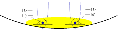
Figure 1: Impurity atoms held by tight confining potentials in a Bose-Einstein condensate. When in internal state $|1\rangle$ the atoms undergo s-wave scattering interactions with the condensate.

In order to derive an effective Hamiltonian for the two impurity atoms it is convenient to first separate the interaction (1) into a mean-field and a fluctuation part

$$\begin{split}\hat{H}_{\mathrm{int}}=&\left|1\right\rangle_{11}\!\left\langle 1\right|\frac{\kappa}{2}\left\langle\hat{C}_{1}(t)\right\rangle+\left|1\right\rangle_{22}\!\left\langle 1\right|\frac{\kappa}{2}\left\langle\hat{C}_{2}(t)\right\rangle\\ &+\sum_{\alpha,\beta}\left|\alpha,\beta\right\rangle\left\langle\alpha,\beta\right|\left(\frac{\kappa_{\alpha}}{2}\hat{B}_{1}(t)+\frac{\kappa_{\beta}}{2}\hat{B}_{2}(t)\right)\,,\end{split}$$ (3)

where

$$\hat{C}_{l}(t)=\int\!\mathrm{d}\mathbf{r}\,\left|\phi_{0}(\mathbf{r}-\mathbf{r}_{l})\right|^{2}\hat{\psi}^{\dagger}(\mathbf{r},t)\hat{\psi}(\mathbf{r},t)\,,$$ (4)

and

$$\hat{B}_{l}(t)=\hat{C}_{l}(t)-\left\langle\hat{C}_{l}(t)\right\rangle\,.$$ (5)

The terms in the first line of eq.(3) result in a mean-field level shift of the internal state $|1\rangle$. They are of no interest in the present discussion and will be absorbed in the free Hamiltonian of the impurity atoms.

We proceed by deriving an equation of motion for the statistical operator of the impurities interacting with the BEC. Within the usual Born approximation and as outlined in Appendix A one finds

$$\partial_{t}\tilde{\varrho}_{10,00} = -\frac{\kappa^{2}}{4\hbar^{2}}\int_{t_{0}}^{t}\!\mathrm{d}t^{\prime}\,\tilde{\varrho}_{10,00}(t^{\prime})\left\langle\tilde{B}_{1}(t)\tilde{B}_{1}(t^{\prime})\right\rangle$$ (6)

$$\partial_{t}\tilde{\varrho}_{01,00} = -\frac{\kappa^{2}}{4\hbar^{2}}\int_{t_{0}}^{t}\!\mathrm{d}t^{\prime}\,\tilde{\varrho}_{01,00}(t^{\prime})\left\langle\tilde{B}_{2}(t)\tilde{B}_{2}(t^{\prime})\right\rangle$$ (7)

$$\partial_{t}\tilde{\varrho}_{11,00} = -\frac{\kappa^{2}}{4\hbar^{2}}\int_{t_{0}}^{t}\!\mathrm{d}t^{\prime}\,\tilde{\varrho}_{11,00}(t^{\prime})\Bigl{\{}\left\langle\tilde{B}_{1}(t)\tilde{B}_{1}(t^{\prime})\right\rangle$$

$$+ \left\langle\tilde{B}_{1}(t)\tilde{B}_{2}(t^{\prime})\right\rangle+\enspace\textrm{terms with}\,\,1\,\leftrightarrow\,2\enspace\Bigr{\}}\,.$$

where the tilde denotes quantities in the interaction picture and the matrix elements of the statistical operator are denoted by $\tilde{\varrho}_{\alpha\beta,\gamma\delta}=\left\langle\alpha\beta,t\right|\tilde{\varrho}\left|\gamma\delta,t\right\rangle$. The correlations $\left\langle\tilde{B}_{l}\tilde{B}_{l^{\prime}}\right\rangle$ are calculated using the standard Bogoliubov approach, i.e. by setting

$$\hat{\psi}(\mathbf{r},t)=\psi_{0}(\mathbf{r})+\hat{\xi}(\mathbf{r},t)$$ (9)

with $\psi_{0}$ being the solution of the Gross-Pitaevskii equation and $\hat{\xi}$ a small operator-valued correction and neglecting higher-order terms in $\hat{\xi}$ (see Appendix B). Within the Bogoliubov approach we disregard terms of the order $\mathcal{O}\left(\xi^{4}\right)$ in $\left\langle\tilde{B}_{i}\tilde{B}_{j}\right\rangle$ and find

$$\left\langle\tilde{B}_{l}(t)\tilde{B}_{l^{\prime}}(t^{\prime})\right\rangle=\left.\sum_{j}\right.^{\prime}\mathrm{e}^{-\frac{i}{\hbar}E_{j}(t-t^{\prime})}S_{j}(l,l^{\prime}).$$ (10)

The $E_{j}$’s are the Bogoliubov energies and

$$\begin{split}&S_{j}(l,l^{\prime})=\int\!\mathrm{d}\mathbf{r}\,\left|\phi_{0}(\mathbf{r}-\mathbf{r}_{l})\right|^{2}\psi_{0}(\mathbf{r})(u_{j}(\mathbf{r})-v_{j}(\mathbf{r}))\\ &\times\int\!\mathrm{d}\mathbf{r}^{\prime}\,\left|\phi_{0}(\mathbf{r}^{\prime}-\mathbf{r}_{l^{\prime}})\right|^{2}\psi_{0}(\mathbf{r}^{\prime})(u^{*}_{j}(\mathbf{r}^{\prime})-v^{*}_{j}(\mathbf{r}^{\prime}))\,.\end{split}$$ (11)

The functions $u_{j}$ and $v_{j}$ are the solutions of the Bogoliubov-de Gennes equations (cf. Appendix B) and the prime at the sum indicates that the ground state is excluded.

A calculation of the correlation functions shows that the often used Markov approximation cannot straight-forwardly applied to eqs.(6-II). Instead we first use a Laplace transformation. Setting $t_{0}=0$ we find

$$\mathcal{L}\left[\tilde{\varrho}_{\alpha\beta,\gamma\delta}(t)\right](p)=\frac{\tilde{\varrho}_{\alpha\beta,\gamma\delta}(0)}{p+\frac{1}{4\hbar^{2}}M_{\alpha\beta,\gamma\delta}(p)}$$ (12)

with

$$\begin{split}&M_{\alpha\beta,\gamma\delta}(p)=\\ &\left.\sum_{j}\right.^{\prime}\left\{S_{j}(1,1)\left(\frac{\kappa^{2}_{\alpha}-\kappa_{\alpha}\kappa_{\gamma}}{p+\frac{i}{\hbar}E_{j}}+\frac{\kappa_{\gamma}^{2}-\kappa_{\alpha}\kappa_{\gamma}}{p-\frac{i}{\hbar}E_{j}}\right)\right.\\ &\phantom{\left.\sum_{j}\right.^{\prime}\{}+S_{j}(1,2)\left(\frac{\kappa_{\alpha}\kappa_{\beta}-\kappa_{\beta}\kappa_{\gamma}}{p+\frac{i}{\hbar}E_{j}}+\frac{\kappa_{\gamma}\kappa_{\delta}-\kappa_{\beta}\kappa_{\gamma}}{p-\frac{i}{\hbar}E_{j}}\right)\\ &\phantom{\left.\sum_{j}\right.^{\prime}\{}+S_{j}(2,1)\left(\frac{\kappa_{\alpha}\kappa_{\beta}-\kappa_{\alpha}\kappa_{\delta}}{p+\frac{i}{\hbar}E_{j}}+\frac{\kappa_{\gamma}\kappa_{\delta}-\kappa_{\alpha}\kappa_{\delta}}{p-\frac{i}{\hbar}E_{j}}\right)\\ &\phantom{\left.\sum_{j}\right.^{\prime}\{}+\left.S_{j}(2,2)\left(\frac{\kappa_{\beta}^{2}-\kappa_{\beta}\kappa_{\delta}}{p+\frac{i}{\hbar}E_{j}}+\frac{\kappa_{\delta}^{2}-\kappa_{\beta}\kappa_{\delta}}{p-\frac{i}{\hbar}E_{j}}\right)\right\}\,.\end{split}$$ (13)

In general, the Laplace transformation (12) cannot be inverted analytically. However, if we are interested only in a coarse-grained time evolution, it is possible to neglect the $p$-dependence of $M_{\alpha\beta,\gamma\delta}$, which amounts to $M_{\alpha\beta,\gamma\delta}(p)\rightarrow M_{\alpha\beta,\gamma\delta}(0)$. In the coarse-grained picture the interaction of the impurity atoms with the condensate simply results into level shifts, i.e.

$$\tilde{\varrho}_{\alpha\beta,\gamma\delta}(t)=\tilde{\varrho}_{\alpha\beta,\gamma\delta}(0)\mathrm{e}^{-i\omega_{\alpha\beta,\gamma\delta}t}.$$ (14)

The corresponding frequencies read

$$\begin{split}&\omega_{\alpha\beta,\gamma\delta}=\frac{1}{4\hbar^{2}i}M_{\alpha\beta,\gamma\delta}(0)=\\ &\frac{1}{4\hbar}\left.\sum_{j}\right.^{\prime}\frac{1}{E_{j}}\left\{S_{j}(1,1)\left(\kappa_{\gamma}^{2}-\kappa_{\alpha}^{2}\right)+S_{j}(2,2)\left(\kappa_{\delta}^{2}-\kappa_{\beta}^{2}\right)\right.\\ &+\left.\left[S_{j}(1,2)+S_{j}(2,1)\right]\left(\kappa_{\gamma}\kappa_{\delta}-\kappa_{\alpha}\kappa_{\beta}\right)\right\}\,.\end{split}$$ (15)

This corresponds to an effective - coarse-grained - Hamiltonian

$$\begin{split}\tilde{H}_{\mathrm{eff}}=&\left|10\right\rangle\left\langle 10\right|\hbar\omega_{10,00}+\left|01\right\rangle\left\langle 01\right|\hbar\omega_{01,00}\\ &+\left|11\right\rangle\left\langle 11\right|\hbar\omega_{11,00}\,.\end{split}$$ (16)

The energy scheme of this Hamiltonian is shown in figure 2. One recognizes from (16) for symmetric impurity locations a level shift

$$\delta = \omega_{10,00}=\omega_{01,00}$$ (17)

$$= -\frac{\kappa^{2}}{4\hbar}{\sum_{j}}^{\prime}S_{j}(l,l)<0$$

of each impurity atom independent of the presence of the other. This level shift is due to the interaction with vacuum fluctuations of the Bogoliubov quasi particles (phonons). In addition there is a conditional level shift due to the exchange of Bogoliubov quasi particles (phonons) between the two impurities:

$$\Delta = \omega_{11,00}-\omega_{10,00}-\omega_{01,00}$$ (18)

$$= -\frac{\kappa^{2}}{4\hbar}\left.\sum_{j}\right.^{\prime}\frac{1}{E_{j}}\left\{S_{j}(1,2)+S_{j}(2,1)\right\}\,.$$

Figure 2: Energy scheme of the effective Hamiltonian for symmetric arrangement of impurity atoms. Here a negative sign of $\Delta$ was assumed although positive values are possible.

It should be noted that the coarse-graining approximation is consitent with the collective level shift only if

$$\Delta\ll\frac{1}{\hbar}\left.\min_{j}\right.^{\prime}\left(E_{j}\right)$$ (19)

where the prime indicates that the ground state is excluded. In the following we will explicitly calculate the levels shifts for a homogeneous condensate, for an ideal condensate in a harmonic trap and a weakly interacting condensate in a trap in the Thomas-Fermi limit.

III Homogeneous Condensate

In this section we calculate the energy shifts $\delta$ and $\Delta$ for the case of an interacting, homogeneous condensate with periodic boundary conditions of spatial periodicity $L_{x}$, $L_{y}$, $L_{z}$, respectively. The solutions of the Bogoliubov-de Gennes equations are then given by plane waves $u_{\mathbf{k}}=(f_{\mathbf{k}}^{+}+f_{\mathbf{k}}^{-})/2$ and $v_{\mathbf{k}}=(f_{\mathbf{k}}^{+}-f_{\mathbf{k}}^{-})/2$ with

$$f^{\pm}_{\mathbf{k}}(\mathbf{r})=\frac{1}{\sqrt{V}}\left(\sqrt{\frac{E_{\mathbf{k}}}{\varepsilon^{0}_{\mathbf{k}}}}\right)^{\pm 1}\mathrm{e}^{i\mathbf{k}\cdot\mathbf{r}}\,.$$ (20)

The wave vectors ${\mathbf{k}}$ have to be chosen in such a way that they fulfill the periodic boundary conditions. Since the $u_{\mathbf{k}}$ and $v_{\mathbf{k}}$’s have to be orthogonal to the ground state the case $\mathbf{k}=0$ is excluded. The Bogoliubov energies are given by

$$E_{\mathbf{k}}=\sqrt{\varepsilon^{0}_{\mathbf{k}}\left(\varepsilon^{0}_{\mathbf{k}}+2gn_{0}\right)}$$ (21)

with $\varepsilon_{\mathbf{k}}^{0}=\hbar^{2}k^{2}/2m_{\mathrm{B}}$. By extending the integral in equation (11) over the whole $\mathbb{R}^{3}$, which is possible due to the effective cut-off provided by the impurity state wavefunctions $\phi_{0}$, one can easily calculate the correlation functions:

$$\begin{split}&\left\langle\tilde{B}_{l}(t)\tilde{B}_{l^{\prime}}(t^{\prime})\right\rangle=\frac{N_{0}}{V^{2}}\left.\sum_{\mathbf{k}}\right.^{\prime}\frac{\varepsilon^{0}_{\mathbf{k}}}{E_{\mathbf{k}}}\exp\left(-\frac{i}{\hbar}E_{\mathbf{k}}(t-t^{\prime})\right)\\ &\qquad\times\exp\left(i\mathbf{k}\cdot\left(\mathbf{r}_{l}-\mathbf{r}_{l^{\prime}}\right)-\frac{z_{0}^{2}\mathbf{k}^{2}}{2}\right)\,.\end{split}$$ (22)

Here $N_{0}$ denotes the number of atoms in the condensate and $V=L_{x}L_{y}L_{z}$. With this one finds

$$\delta = -\frac{\kappa^{2}N_{0}}{4\hbar V^{2}}{\sum_{\mathbf{k}}}^{\prime}\frac{\varepsilon_{\mathbf{k}}^{0}}{E^{2}_{\mathbf{k}}}\exp\left(-\frac{z_{0}^{2}{k}^{2}}{2}\right)$$ (23)

$$\Delta = -\frac{\kappa^{2}N_{0}}{2\hbar V^{2}}{\sum_{\mathbf{k}}}^{\prime}\frac{\varepsilon_{\mathbf{k}}^{0}}{E^{2}_{\mathbf{k}}}\cos\left(\mathbf{k}\cdot\Delta{\mathbf{r}}\right)\exp\left(-\frac{z_{0}^{2}{k}^{2}}{2}\right),\,\,$$ (24)

where $\Delta{\mathbf{r}}={\mathbf{r}}_{1}-{\mathbf{r}}_{2}$. The sum over the Bogoliubov quasi momenta converges due to the exponential term which effectively cuts off momenta with $k\gg 1/z_{0}$. Obviously $2\delta=\Delta$ for $\mathbf{r}_{1}=\mathbf{r}_{2}$ and $|\Delta|\leq 2|\delta|$. The conditional energy shift $\Delta$ is shown in figure 3. For very small distances of the impurities $\Delta$ is negativ and its absolute value approaches its maximum, i.e. that of $2\delta$. For increasing distance the value of $\Delta$ increases monotonously and eventually changes its sign. The monotonous increase would correspond to an attractive force between the impurity atoms if they could move freely. One recognizes, that for larger values of the dimensionless interaction parameter $K\sim g$ the energy shift decreases and the spatial dependence becomes less pronounced. This can be explained by the increasing self-energy of the Bogoliubov excitations.

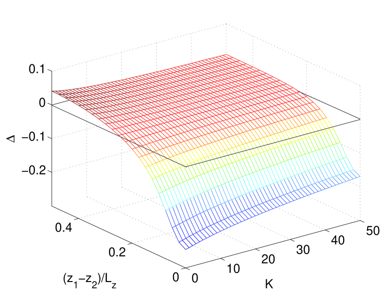
Figure 3: Energy shift in units of $\kappa^{2}N_{0}m_{\mathrm{B}}L_{z}^{2}/\hbar^{3}V^{2}$ for two impurities in a homogeneous condensate with periodic boundary conditions. The interaction of BEC atoms is characterized by the dimensionless parameter $K=gN_{0}2m_{\mathrm{B}}L_{z}^{2}/\hbar^{2}V$. The impurities are located on the $z$-axis, $L_{x}=L_{y}=0.5L_{z}$, and $z_{0}=0.05L_{z}$.

It is also very instructive to consider the dependence of the conditional level shift $\Delta$ on the condensate geometry, i.e. on the ratio $L_{\mathrm{rad}}/L_{z}$, where $L_{\mathrm{rad}}=L_{x}=L_{y}$. This is illustrated in figure 4. One recognizes that the absolute value of the energy shift increases as the ratio $L_{\mathrm{rad}}/L_{z}$ decreases. Thus the energy shift is largest for a highly non-symmetric geometry of the BEC. The strongest effect is thus to be expected in a quasi one-dimensional condensate. For this reason we will investigate in the following section the energy shift in the case of a BEC in a harmonic trap only for a one-dimensional condensate.

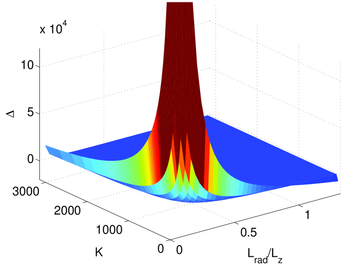
Figure 4: Influence of condensate geometry on energy shift in a box with periodic boundary conditions. $\Delta$ is in units of $\kappa^{2}2m_{\mathrm{B}}/4\hbar^{3}$, $K$ is defined as in figure 3. The impurities are located on the $z$-axis with a distance of $0.5L_{z}$. $L_{z}=12\cdot 10^{-6}\mathrm{m}$, and $L_{x}=L_{y}$ has been varied.

IV 1-D condensate in a trap

In this section we consider a quasi one-dimensional condensate confined in an harmonic trap $V_{\mathrm{ext}}=m_{\mathrm{B}}\omega_{\mathrm{B}}^{2}z^{2}/2$. We first consider the case of an ideal, i.e. noninteracting gas. In this case the solutions of the Gross-Pitaevskii equation and the Bogoliubov-de Gennes equations are just the solutions of the harmonic oscillator:

$$\psi_{0}(z)=\sqrt{\frac{N_{0}}{\sqrt{\pi}z_{\mathrm{B}}}}\mathrm{e}^{-{z^{2}}/{2z_{\mathrm{B}}^{2}}}$$ (25)

$$u_{j}(z)=\frac{1}{\sqrt{2^{j}j!\sqrt{\pi}z_{\mathrm{B}}}}\mathrm{e}^{-{z}^{2}/2z_{\mathrm{B}}^{2}}H_{j}\left(\frac{z}{z_{\mathrm{B}}}\right)$$ (26)

$$v_{j}(z)=0$$ (27)

$$E_{j}=j\hbar\omega_{\mathrm{B}}\,.$$ (28)

Here $z_{\mathrm{B}}=\sqrt{\hbar/m\omega_{\mathrm{B}}}$ is the ground-state width of the 1-D harmonic trap. By calculating the integrals in equation (11) one finds

$$\begin{split}\Delta=-\frac{\kappa_{\mathrm{1D}}^{2}}{2\hbar}\sum_{\nu=1}^{\infty}&\frac{1}{\hbar\nu\omega_{\mathrm{B}}}\frac{N_{0}\exp\left(-\check{z}_{1}^{2}-\check{z}_{2}^{2}\right)}{\pi(z_{0}^{2}+z_{\mathrm{B}}^{2})}\frac{\check{z}^{\nu}}{2^{\nu}\nu!}\\ &\times H_{\nu}\left(\check{z}_{1}\right)H_{\nu}\left(\check{z}_{2}\right)\,,\end{split}$$ (29)

where $\check{z}=z_{\mathrm{B}}^{2}/(z_{\mathrm{B}}^{2}+z_{0}^{2})$ and $\check{z}_{l}={z_{l}}/{\sqrt{z_{\mathrm{B}}^{2}+z_{0}^{2}}}$. We also have introduced the one-dimensional coupling constant $\kappa_{\mathrm{1D}}=\kappa/(2\pi a_{\bot}^{2})$ with the radial confinement $a_{\bot}^{2}=\hbar/m_{\mathrm{B}}\omega_{\bot}$. The conditional level shift is shown in figure 5 for different widths $z_{0}$ of the impurity traps. As expected the shape of the curves coincides for distances larger than the ground state width of the impurity traps. Distances smaller than $z_{0}$ are excluded because we have assumed that there is no direct scattering interaction between the impurity atoms.

It is interesting to note that different from the case of a condensate in a box, the force between the impurities is not always attractive. One recognizes that this is only the case if the distance is sufficiently small. If the distance is larger than a certain value, in our case $\check{z}_{1}-\check{z}_{2}\approx 2\cdot 0.6$, the force becomes repulsive.

Figure 5: Energy shift $\Delta$ in an ideal 1-D condensate as function of impurity distance for different ratios of $z_{\mathrm{B}}/z_{0}$. The shift is given in units of $\kappa_{\mathrm{1D}}^{2}N_{0}/2\hbar^{2}\omega_{\mathrm{B}}\pi\left(z_{\mathrm{B}}^{2}+z_{0}^{2}\right)$. The inset shows a magnification for small distances. Here $\check{z}_{1}=-\check{z}_{2}$.

We now consider the case of a weakly interacting 1-D gas. In order to solve the Gross-Pitaevskii equation we make use of the Thomas-Fermi (TF) approximation. Although the results obtained in this way cannot be smoothly connected to the ideal-condensate case, the TF approximation allows to derive a compact expression for the level shift. The TF condensate wavefunction is given by

$$\psi_{0}(z)=\sqrt{\frac{\mu}{g_{\mathrm{1D}}}\left(1-\frac{z^{2}}{R_{\mathrm{TF}}^{2}}\right)}\,,$$ (30)

where the TF radius is given by $R_{\mathrm{TF}}=\sqrt{2\mu/m_{\mathrm{B}}\omega_{\mathrm{B}}^{2}}$. $\mu$ denotes the chemical potential and the one dimensional interaction parameter $g_{\mathrm{1D}}$ is defined analogous to $\kappa_{\mathrm{1D}}$. To solve the Bogoliubov-de Gennes equations analytically further approximtions are needed as discussed in Oehberg-PRA-1997 . We here take over the results for the functions $f^{\pm}_{j}$ obtained in Petrov-PRL-2000 :

$$f^{\pm}_{j}(z)=\sqrt{\frac{2j+1}{2R_{\mathrm{TF}}}}\left[\frac{2\mu}{E_{j}}\left(1-\frac{z^{2}}{R_{\mathrm{TF}}^{2}}\right)\right]^{\pm\frac{1}{2}}P_{j}\left(\frac{z}{R_{\mathrm{TF}}}\right)$$ (31)

with the energies $E_{j}=\hbar\omega_{\mathrm{B}}\sqrt{j(j+1)/2}$. The $P_{j}$ are Legendre polynomials. Using the completeness of the Legendre polynomials one can explicitely evaluate expression (18). One finds that the sum including the $j=0$ term vanishes if the overlap of the impurity wavefunctions is negligible:

$$\begin{split}&\sum_{j=0}^{\infty}\frac{S_{j}(1,2)}{E_{j}}\\ &\quad=-\frac{1}{2g_{\mathrm{1D}}}\int\!\mathrm{d}z\,\left|\phi_{0}(z-z_{1})\right|^{2}\left|\phi_{0}(z-z_{2})\right|^{2}\approx 0\,.\end{split}$$ (32)

Thus the energy shift (18) is determined only by the $j=0$ term which yields the simple expression :

$$\Delta=\frac{\kappa_{\mathrm{1D}}^{2}}{8\hbar R_{\mathrm{TF}}g_{\mathrm{1D}}}\,.$$ (33)

This result does not depend on the distance of the impurity atoms which is due to the Thomas-Fermi approximation. The shift is always positive and becomes larger for smaller interactions in the BEC and for larger 1D confinement. It is instructive to express $\Delta$ in terms of the impurity-BEC stattering length $a_{\mathrm{i}}$ and the BEC scattering length $a$. One finds

$$\Delta=\frac{\omega_{\perp}}{4}\frac{m_{\mathrm{B}}^{2}}{m_{\mathrm{i}}^{2}}\frac{a_{\mathrm{i}}^{2}}{R_{\mathrm{TF}}a}$$ (34)

Here we have $m_{\mathrm{i}}=2m_{\mathrm{B}}m_{\mathrm{S}}/(m_{\mathrm{B}}+m_{\mathrm{S}})$. Thus assuming a tight transversal confinement with $\omega_{\perp}=2\pi\times 10^{4}$ Hz, a large scattering length between impurities and BEC $a_{\mathrm{i}}=200$nm, a small scattering within the BEC $a=5$ nm, a small trap with $R_{\mathrm{TF}}=20\mu$m, and $m_{\mathrm{S}}\approx m_{\mathrm{B}}$ one finds a conditional frequency shift of $2\pi\times 10^{3}$ Hz.

As shown in Appendix C the result of equation (33) should be valid as long as the following conditions are fulfilled

$$\frac{z_{1}-z_{2}}{R_{\mathrm{TF}}}\gg\pi\sqrt{\frac{\zeta}{2}}$$ (35)

$$\frac{\delta r}{R_{\mathrm{TF}}}\gg\max\left\{\sqrt{\zeta},\frac{z_{0}}{R_{\mathrm{TF}}}\right\}\,.$$ (36)

Here, $\delta r$ denotes the distance of one of the impurities to the edge of the condensate and $\zeta=\hbar\omega_{\mathrm{B}}/2\mu$ is the Thomas-Fermi parameter. Furthermore the interaction strength of the condensate has to fulfill the condition

$$g_{\mathrm{1D}}\gg\frac{2\hbar\omega_{\mathrm{B}}R_{\mathrm{TF}}}{3N_{0}}\,.$$ (37)

Hence, we have the restriction

$$\Delta\ll\min\left\{\omega_{\mathrm{B}},\frac{3N_{0}\kappa_{\mathrm{1D}}^{2}}{16\hbar^{2}R^{2}_{\mathrm{TF}}\omega_{\mathrm{B}}}\right\}\,.$$ (38)

V Conclusions

In the present paper we have analyzed the interaction of impurity atoms in a Bose-Einstein condensate localized at specific positions by tight confining potentials. It was shown that in addition to the level shift caused by s-wave scattering with the macroscopic condensate field there are also contributions from the interaction with vacuum fluctuations of the Bogoliubov phonons. The self- and conditonal energy shifts were calculated for a BEC in a box with periodic boundary conditions. It was shown that size and sign of the conditional energy shift depends on the separation of the impurities and is largest for a highly anisotropic condensate geometry and for small interactions within the condensate. With increasing interaction of the condensate atoms the spatial dependence becomes less and less pronounced. Motivated by these findings the level shift in a quasi one-dimensional harmonic trap was calculated. In the Thomas-Fermi limit a rather simple analytic expression was obtained from a Bogoliubov approach. For small trap sizes a conditional frequency shift in the range of several kHz seems feasible which could be of interest for the implementation of a quantum phase gate.

Appendix A Derivation of the equation of motion for the statistical operator

The total statistical operator of both the condensate and the impurities is denoted by $\hat{\chi}$. Its time evolution is then given by the Liouville-von Neumann equation $i\hbar\partial_{t}\hat{\chi}(t)=\left[\hat{H},\hat{\chi}(t)\right]$, where $\hat{H}=\hat{H}_{\mathrm{B}}+\hat{H}_{\mathrm{S}}+\hat{H}_{\mathrm{int}}$ is the Hamiltonian of the whole system, with $\hat{H}_{\mathrm{B}}$ being the Hamiltonian of the condensate, $\hat{H}_{\mathrm{S}}$ that of the impurities and $\hat{H}_{\mathrm{int}}$ the interaction. Changing into the interaction picture yields

$$i\hbar\partial_{t}\tilde{\chi}(t)=\left[\tilde{H}_{\mathrm{int}}(t),\tilde{\chi}(t)\right]\,.$$ (39)

Formal integration and resubstitution leads to

$$\begin{split}i\hbar\partial_{t}\tilde{\chi}(t)=&\left[\tilde{H}_{\mathrm{int}}(t),\tilde{\chi}(t_{0})\right]\\ &+\frac{1}{i\hbar}\int_{t_{0}}^{t}\mathrm{d}t^{\prime}\left[\tilde{H}_{\mathrm{int}}(t),\left[\tilde{H}_{\mathrm{int}}(t^{\prime}),\tilde{\chi}(t^{\prime})\right]\right]\,.\end{split}$$ (40)

Here, $t_{0}$ is the time when the interaction starts. The statistical operator for the impurity atoms can be obtained by tracing out the condensate, i.e. $\tilde{\varrho}(t)=\mathrm{Tr}_{\mathrm{B}}\left[\tilde{\chi}(t)\right]$. This yields

$$\begin{split}&i\hbar\partial_{t}\tilde{\varrho}(t)=\mathrm{Tr}_{\mathrm{B}}\left(\left[\tilde{H}_{\mathrm{int}}(t),\tilde{\chi}(t_{0})\right]\right)\\ &\quad+\frac{1}{i\hbar}\int_{t_{0}}^{t}\!\mathrm{d}t^{\prime}\,\mathrm{Tr}_{\mathrm{B}}\left(\left[\tilde{H}_{\mathrm{int}}(t),\left[\tilde{H}_{\mathrm{int}}(t^{\prime}),\tilde{\chi}(t^{\prime})\right]\right]\right)\,.\end{split}$$ (41)

Following the standard approach we assume that the influence of the impurity atoms on the condensate can be neglected and that the statistical operator of the whole system seperates as

$$\tilde{\chi}(t)=\tilde{\varrho}(t)\otimes\tilde{\varrho}_{\mathrm{B}}(t)+\tilde{\chi}_{\mathrm{corr}}(t)\approx\tilde{\varrho}(t)\otimes\tilde{\varrho}_{\mathrm{B}}(t_{0})\,.$$ (42)

Furthermore since we have incorporated the mean-field contribution to the free Hamiltonian of the impurities, the expectation value of the interaction Hamiltonian vanishes. , i.e. $\mathrm{Tr}_{\mathrm{B}}\left(\tilde{\varrho}_{\mathrm{B}}(t_{0})\tilde{H}_{\mathrm{int}}(t)\right)=0$. With these approximations we obtain

$$\begin{split}\partial_{t}\tilde{\varrho}(t)=&-\frac{1}{\hbar^{2}}\int_{t_{0}}^{t}\!\mathrm{d}t^{\prime}\,\\ &\cdot\mathrm{Tr}_{\mathrm{B}}\left(\left[\tilde{H}_{\mathrm{int}}(t),\left[\tilde{H}_{\mathrm{int}}(t^{\prime}),\tilde{\varrho}(t^{\prime})\otimes\tilde{\varrho}_{\mathrm{B}}(t_{0})\right]\right]\right)\,.\end{split}$$ (43)

The interaction Hamiltonian in the interaction picture can be expressed as

$$\tilde{H}_{\mathrm{int}}(t)=\sum_{\alpha,\beta}|\alpha\beta,t\rangle\langle\alpha\beta,t|\left(\frac{\kappa_{\alpha}}{2}\tilde{B}_{1}(t)+\frac{\kappa_{\beta}}{2}\tilde{B}_{2}(t)\right)\,.$$ (44)

where

$$|\alpha\beta,t\rangle\langle\alpha\beta,t|=\mathrm{e}^{\frac{i}{\hbar}\left(\hat{H}_{\mathrm{S}}+\hat{H}_{\mathrm{B}}\right)t}\left|\alpha\beta\right\rangle\left\langle\alpha\beta\right|\mathrm{e}^{-\frac{i}{\hbar}\left(\hat{H}_{\mathrm{S}}+\hat{H}_{\mathrm{B}}\right)t}.$$ (45)

Substituting this into eq. (43) yields

$$\begin{split}\partial_{t}\tilde{\varrho}_{\alpha\beta,\gamma\delta}(t)=-\frac{1}{4\hbar^{2}}\int_{t_{0}}^{t}\!\mathrm{d}t^{\prime}\,\tilde{\varrho}_{\alpha\beta,\gamma\delta}(t^{\prime})&\left(\left\langle\tilde{B}_{1}(t)\tilde{B}_{1}(t^{\prime})\right\rangle\left(\kappa^{2}_{\alpha}-\kappa_{\alpha}\kappa_{\gamma}\right)+\left\langle\tilde{B}_{1}(t)\tilde{B}_{2}(t^{\prime})\right\rangle\left(\kappa_{\alpha}\kappa_{\beta}-\kappa_{\beta}\kappa_{\gamma}\right)\right.\\ &+\left\langle\tilde{B}_{2}(t)\tilde{B}_{1}(t^{\prime})\right\rangle\left(\kappa_{\alpha}\kappa_{\beta}-\kappa_{\alpha}\kappa_{\delta}\right)+\left\langle\tilde{B}_{2}(t)\tilde{B}_{2}(t^{\prime})\right\rangle\left(\kappa_{\beta}^{2}-\kappa_{\beta}\kappa_{\delta}\right)\\ &+\left\langle\tilde{B}_{1}(t^{\prime})\tilde{B}_{1}(t)\right\rangle\left(\kappa_{\gamma}^{2}-\kappa_{\alpha}\kappa_{\gamma}\right)+\left\langle\tilde{B}_{1}(t^{\prime})\tilde{B}_{2}(t)\right\rangle\left(\kappa_{\gamma}\kappa_{\delta}-\kappa_{\beta}\kappa_{\gamma}\right)\\ &\left.+\left\langle\tilde{B}_{2}(t^{\prime})\tilde{B}_{1}(t)\right\rangle\left(\kappa_{\gamma}\kappa_{\delta}-\kappa_{\alpha}\kappa_{\delta}\right)+\left\langle\tilde{B}_{2}(t^{\prime})\tilde{B}_{2}(t)\right\rangle\left(\kappa_{\delta}^{2}-\kappa_{\beta}\kappa_{\delta}\right)\right)\,.\end{split}$$ (46)

Appendix B Bogoliubov theory

In this appendix we briefly summarize the main results of the Bogoliubov approach. We start with the hamiltonian of the Bose gas in $s$-wave-scattering approximation

$$\begin{split}\hat{H}_{\mathrm{B}}=&\int\!\mathrm{d}\mathbf{r}\,\hat{\psi}^{\dagger}(\mathbf{r})\left(-\frac{\hbar^{2}}{2m_{\mathrm{B}}}\Delta+V_{\mathrm{ext}}(\mathbf{r})-\mu\right)\hat{\psi}(\mathbf{r})\\ &+\frac{g}{2}\int\!\mathrm{d}\mathbf{r}\,\hat{\psi}^{\dagger}(\mathbf{r})\hat{\psi}^{\dagger}(\mathbf{r})\hat{\psi}(\mathbf{r})\hat{\psi}(\mathbf{r})\,.\end{split}$$ (47)

The field operator $\hat{\psi}$ of the condensate is then devided into a $\mathbb{C}$-number function $\psi_{0}$ which represents the condensed part of the Bose-gas and an operator $\hat{\xi}$ of quantum fluctuations: $\hat{\psi}({\mathbf{r}})=\psi_{0}({\mathbf{r}})+\hat{\xi}({\mathbf{r}})$. The wavefunction of the condensate is given by the Gross-Pitaevskii equation

$$\left(-\frac{\hbar^{2}}{2m_{\mathrm{B}}}\Delta+V_{\mathrm{ext}}(\mathbf{r})-\mu+g\left|\psi_{0}(\mathbf{r})\right|^{2}\right)\psi_{0}(\mathbf{r})=0\,.$$ (48)

By plugging this into the Hamiltonian and neglecting terms of the order $\mathcal{O}(\hat{\xi}^{3})$ and higher one gets

$$\begin{split}\hat{H}_{\mathrm{B}}\approx H_{\mathrm{B}}^{0}+\int\!&\mathrm{d}\mathbf{r}\,\biggl{\{}\hat{\xi}^{\dagger}(\mathbf{r})\left(-\frac{\hbar^{2}}{2m_{\mathrm{B}}}\Delta+V_{\mathrm{ext}}(\mathbf{r})-\mu\right)\hat{\xi}(\mathbf{r})\\ &+\frac{g}{2}\left(4\left|\psi_{0}(\mathbf{r})\right|^{2}\hat{\xi}^{\dagger}(\mathbf{r})\hat{\xi}(\mathbf{r})\right.\\ &\left.+\psi_{0}^{2}(\mathbf{r})\hat{\xi}^{\dagger}(\mathbf{r})\hat{\xi}^{\dagger}(\mathbf{r})+\left.\psi_{0}^{*}\right.^{2}(\mathbf{r})\hat{\xi}(\mathbf{r})\hat{\xi}(\mathbf{r})\right)\biggr{\}}\,.\end{split}$$ (49)

The terms linear in $\hat{\xi}$ vanish because of the Gross-Pitaevskii equation. The term $H_{\mathrm{B}}^{0}$ does not depend on operators and is without consequence. In order to diagonalize the Hamiltonian we employ the Bogoliubov ansatz

$$\hat{\xi}(\mathbf{r})=\left.\sum_{\nu}\right.^{\prime}u_{\nu}(\mathbf{r})\hat{b}_{\nu}-v_{\nu}^{*}(\mathbf{r})\hat{b}_{\nu}^{\dagger}$$ (50)

$$\hat{\xi}^{\dagger}(\mathbf{r})=\left.\sum_{\nu}\right.^{\prime}u_{\nu}^{*}(\mathbf{r})\hat{b}_{\nu}^{\dagger}-v_{\nu}(\mathbf{r})\hat{b}_{\nu}\,.$$ (51)

Here, $\hat{b}_{\nu}^{\dagger}$ and $\hat{b}_{\nu}$ are bosonic creation and anihilation operators of the Bogoliubov quasi-particles. The prime at the sum indicates that the ground state is excluded in the summation. If the wave functions $u_{\nu}$ and $v_{\nu}$ fulfill the Bogoliubov-de Gennes equations ($\psi_{0}$ is taken to be real)

$$\left[-\frac{\hbar^{2}\Delta}{2m_{\mathrm{B}}}+V_{\mathrm{ext}}(\mathbf{r})-\mu\right]u_{\nu}+g\left|\psi_{0}\right|^{2}\left(2u_{\nu}-v_{\nu}\right)=E_{\nu}u_{\nu}$$ (52)

$$\left[-\frac{\hbar^{2}\Delta}{2m_{\mathrm{B}}}+V_{\mathrm{ext}}(\mathbf{r})-\mu\right]v_{\nu}+g\left|\psi_{0}\right|^{2}\left(2v_{\nu}-u_{\nu}\right)=-E_{\nu}v_{\nu}\,,$$ (53)

with the normalization

$$\int\left\{u_{\nu}(\mathbf{r})u^{*}_{\nu^{\prime}}(\mathbf{r})-v_{\nu}(\mathbf{r})v^{*}_{\nu^{\prime}}(\mathbf{r})\right\}\mathrm{d}\mathbf{r}=\delta_{\nu\nu^{\prime}}$$ (54)

$$\int\left\{v_{\nu}(\mathbf{r})u_{\nu^{\prime}}(\mathbf{r})-u_{\nu}(\mathbf{r})v_{\nu^{\prime}}(\mathbf{r})\right\}\mathrm{d}\mathbf{r}=0\,,$$ (55)

the Hamiltonian takes the very simple form

$$\hat{H}_{\mathrm{B}}=H^{0}_{\mathrm{B}}-\left.\sum_{\nu}\right.^{\prime}E_{\nu}\int\left|v_{\nu}(\mathbf{r})\right|^{2}\mathrm{d}\mathbf{r}+\left.\sum_{\nu}\right.^{\prime}E_{\nu}\hat{b}_{\nu}^{\dagger}\hat{b}_{\nu}\,.$$ (56)

With this the operators $\tilde{\xi}$ in the interaction picture can easily be calculated

$$\tilde{\xi}(\mathbf{r},t)=\left.\sum_{\nu}\right.^{\prime}u_{\nu}(\mathbf{r})\hat{b}_{\nu}\mathrm{e}^{-iE_{\nu}t/\hbar}-v_{\nu}^{*}(\mathbf{r})\hat{b}_{\nu}^{\dagger}\mathrm{e}^{+iE_{\nu}t/\hbar}\,.$$ (57)

Appendix C Validity of eq. (33)

In order to estimate the range of validity of the expression for the conditional shift in TF approximation, eq. (33), we start with the expression (see also eq.(11)

$$\begin{split}\sum_{j=0}^{M}\frac{S_{j}(1,2)}{E_{j}}=&\sum_{j=0}^{M}\frac{1}{E_{j}}\int_{-R_{\mathrm{TF}}}^{R_{\mathrm{TF}}}\!\mathrm{d}z\,\left|\phi_{0}(z-z_{1})\right|^{2}\psi_{0}(z)f^{-}_{j}(z)\\ &\times\int_{-R_{\mathrm{TF}}}^{R_{\mathrm{TF}}}\!\mathrm{d}z^{\prime}\left|\phi_{0}(z^{\prime}-z_{2})\right|^{2}\psi_{0}(z^{\prime})f^{-}_{j}(z^{\prime})\,,\end{split}$$ (58)

where $f^{-}_{j}=u_{j}-v_{j}$. By using (31) we find

$$\begin{split}&\sum_{j=0}^{M}\frac{S_{j}(1,2)}{E_{j}}\sim\int_{-R_{\mathrm{TF}}}^{R_{\mathrm{TF}}}\!\mathrm{d}z\,\int_{-R_{\mathrm{TF}}}^{R_{\mathrm{TF}}}\!\mathrm{d}z^{\prime}\,\\ &\qquad\times\left|\phi_{0}(z-z_{1})\right|^{2}\left|\phi_{0}(z^{\prime}-z_{2})\right|^{2}f_{\mathrm{P}}^{M}\left(\frac{z}{R_{\mathrm{TF}}},\frac{z^{\prime}}{R_{\mathrm{TF}}}\right)\end{split}$$ (59)

5 where we have introduced

$$f_{\mathrm{P}}^{M}(x,x^{\prime})=\sum_{n=0}^{M}\frac{2n+1}{2}P_{n}(x)P_{n}(x^{\prime})\,.$$ (60)

If $M\rightarrow\infty$ the sum approaches the $\delta$-function and we obtain equation (LABEL:HmWW1Dfast0). On the other hand the solutions (31) of the Bogoliubov-de Genne equations used here are only valid for Oehberg-PRA-1997

$$\frac{\delta r}{R_{\mathrm{TF}}}\gg\max\left[\frac{\sqrt{M(M+1)}\zeta}{\sqrt{2}},\sqrt{\frac{\sqrt{2}\zeta}{\sqrt{M(M+1)}}}\,\right],$$ (61)

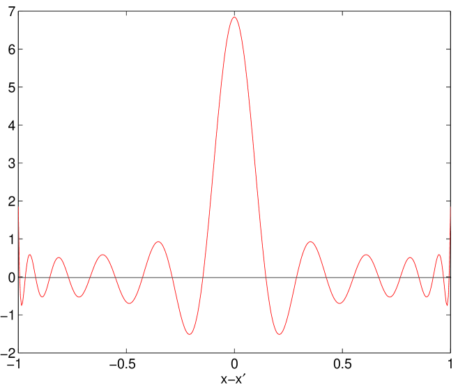
Figure 6: Picture of $f_{\mathrm{P}}^{M}$ for $M=20$.

where $\delta r$ is the distance from the edge of the condensate. This implies $M\ll\sqrt{2}\delta r/R_{\mathrm{TF}}\zeta$ and with $\delta r\gg R_{\mathrm{TF}}\sqrt{\zeta}$, also following from eq.(61) we arrive at $M\ll\sqrt{\frac{2}{\zeta}}$. Thus the limit $M\rightarrow\infty$ cannot be taken in (60). Nevertheless even for a finite but sufficiently large upper limit of summation $M$ the sum is to a good approximation zero as can be seen as follows: In figure 6 $f_{\mathrm{P}}^{20}$ is shown. One recognizes a pronounced central maximum. The first integral over $z$ in equation (59) only contributes if there is an overlapp of the maximum of $f_{\mathrm{P}}^{M}$ and the ground state $\phi_{0}(z-z_{1})$. The same holds for the second integral over $z^{\prime}$ and $\phi_{0}(z^{\prime}-z_{2})$. Hence, equation (59) vanishes if the distance of the impurities is much bigger than the width of the central maximum. We thus need to estimate the width of this central peak. With the Stirling formula one finds asymptotically for large (and even) $M$

$$f^{M}_{\mathrm{P}}(0,0)\approx\frac{M}{\pi}\,.$$ (62)

Since $\int f^{M}_{\mathrm{P}}(0,s)\,\mathrm{d}s=1$ the width of the central peak can be approximated as $\Delta s=\pi/M$. This finally yields the condition

$$\frac{z_{1}-z_{2}}{R_{\mathrm{TF}}}\gg\frac{\pi}{M}\gg\pi\sqrt{\frac{\zeta}{2}}$$ (63)

for which the sum in (59) is approximately 0. It should be noted that we have assumed the Thomas-Fermi limit $\zeta\ll 1$, which is essential for the analytic solution of the Gross-Pitaevskii and Bogoliubov-de Gennes equations.

References

(1) for a review see: Nature 416, 205-246 (2002).
(2)
N. Schlosser, G. Reymaond, I. Protsenko, and P. Grangier,
Nature 411, 1024 (2001).
(3) R. B. Diener, B. Wu, M. G. Raizen and Q. Niu,
Phys. Rev. Lett. 89, 070401 (2002).
(4) R. Dumke, M. Volk, T. Münther,
F.B.J. Buchkremer, G. Birkl, and
W. Ertmer, Phys. Rev. Lett. 89, 097903 (2002).
(5) C. Orzel, A. K. Tuchmann, M. L. Fenselau,
M. Yasuda, and M. A. Kasevich, Science 291, 2386 (2001).
(6)
M. Greiner, O. Mandel, T. Esslinger, T. Hänsch,
and I. Bloch, Nature 415, 39 (2002).
(7)
O. Mandel, M. Greiner, A. Widera,
T. Rom, T. W. Hänsch, I. Bloch, Nature 425, 937 (2003).
(8) see e.g.: R. Folmann, P. Kruger, J. Schmiedmayer,
J. Denschlag, and C. Henkel, Adv. At. Mol. Opt. Phys. 48, 263 (2002)
and references.
(9) see e.g.:
D. Bouwmeester, A. Ekert and A. Zeilinger (Eds.),
“The Physics of Quantum Information” (Springer, Berlin, 2000)
(10) A. Recati, P. O. Fedichev, W. Zwerger,
J. von Delft, and P. Zoller, cond-mat/0404533.
(11) A. Micheli, A. J. Daley, D. Jaksch, and
P. Zoller, quant-ph/0406020.
(12) P. Öhberg, E. L. Surkov, L. Tittonen, S. Stenholm,
M. Wilkens, and G. V. Shlyapnikov,
Phys. Rev. A 56, R3346 (1997).
(13) D. S. Petrov, G. V. Shlyapnikov, and
J. T. M. Walraven, Phys. Rev. Lett. 85, 3745 (2000).