Coherence in scale-free networks of chaotic maps

Abstract

We study fully synchronized states in scale-free networks of chaotic logistic maps as a function of both dynamical and topological parameters. Three different network topologies are considered: (i) random scale-free topology, (ii) deterministic pseudo-fractal scale-free network, and (iii) Apollonian network. For the random scale-free topology we find a coupling strength threshold beyond which full synchronization is attained. This threshold scales as $k^{-\mu}$, where $k$ is the outgoing connectivity and $\mu$ depends on the local nonlinearity. For deterministic scale-free networks coherence is observed only when the coupling strength is proportional to the neighbor connectivity. We show that the transition to coherence is of first-order and study the role of the most connected nodes in the collective dynamics of oscillators in scale-free networks.

I Introduction and model

Recently, intensive research on the structure and dynamics of networks has provided insight for many systems where they arise naturally livro ; albert02 ; dorogovtsevrev . Complex networks appear in a wide variety of fields ranging from lasers meucci02 , granular media snoeijer04 ; otto03 , quantum transport texier04 , colloidal suspensions tanaka04 , electrical circuits almond04 , and time series analysis small02 , to heart rhythms stewart04 , epidemics moreno04 ; dezso02 , protein folding compiani04 , and locomotion zhaoping04 among others livro ; albert02 ; dorogovtsevrev .

From the mathematical point of view, a network is a graph, composed by nodes or vertices and by their connections or edges albert02 . When studying network dynamics one frequently assumes a regular structure where each node evolves according to some more or less complicated dynamics, typically fixed points lind04 , limit cycles strogatz00 or chaotic attractors pecora97 ; anteneodo04 . When studying network structure, one usually neglects node dynamics and all complexity is introduced by the way nodes are connected to each other, i.e. by the network topology. With respect to their topology, networks are usually divided into three large classes albert02 : random networks, where all the nodes are randomly connected erdos , small-world networks introduced recently by Watts and Strogatz strogatz01 ; watts98 as a middle ground between regular and random networks, and the scale-free networks (e.g. Barabási and Albert barabasi99 ), where growth and preferential attachment are considered.

The next logical step toward real network dynamics is to consider simultaneously structural and dynamic complexity. One important question addressed in this context is to know if synchronization between oscillators in such complex topologies would appear and under which conditions it prevails. In fact, coherent behavior of oscillator networks with complex topologies has been studied for the random topology manrubia99 ; jost01 and small-world topology nishikawa03 ; barahona02 ; lago-fernandez00 ; hong04 . However, apart from a few exceptions jost01 ; jostalso ; ieee , there is a quite general lack of studies tackling synchronization of chaotic oscillators in scale-free topologies.

In this paper we present detailed results concerning synchronization in oscillator networks with scale-free topologies. Our purpose is to determine under which conditions scale-free topologies enable the emergence of coherent behavior. As a general result, we present evidences that the transition to synchronization is of first-order. Our model reads

$$x_{t+1,i}=(1-\varepsilon)f(x_{t,i})+\frac{\varepsilon}{{\cal N}_{i}}\sum_{j\in{\cal K}_{i}}k_{j}^{\alpha}f(x_{t,j}),$$ (1)

where $i=1,\dots,L$ and $t$ label discrete space and time respectively, $L$ being the total number of oscillators, $0\leq\varepsilon\leq 1$ is the coupling parameter, ${\cal K}_{i}$ represents the set of labels of the neighbors of node $i$, $k_{i}$ represents the number of such neighbors, and ${\cal N}_{i}=\sum_{j\in{\cal K}_{i}}k_{j}^{\alpha}$ normalizes the interaction term in Eq. (1). The function $f(x)$ is a continuous function governing node dynamics when connections are absent. Here we choose the well-known quadratic map $f(x)=1-ax^{2}$, where the free parameter $a$ is restricted to the interval $-0.25\leq a\leq 2$ and contains all possible dynamical regimes from a fixed point (e.g. a=0) to fully developed chaotic orbits (e.g. $a=2$). The parameter $\alpha$ is a real number controlling the homogeneity in the coupling: positive values of $\alpha$ enhance the coupling strength with sites having larger number of neighbors, while negative values favor sites having less neighbors. For $\alpha=0$ the coupling between each site and its neighborhood is homogeneous, i.e. it is independent on the coordination.

The linear stability of the coherent states $x_{t,i}=X,\forall i$ is governed by the variational equations of Eq. (1), whose diagonal form reads pecora98 ; fink00 ; manrubiabook

$$\xi_{t+1,i} = \exp{\left(\Lambda(\varepsilon\lambda_{i})\right)}\xi_{t,i}$$ (2)

$$= \left[Df(X)-\varepsilon\lambda_{i}Df(X)\right]\xi_{t,i},$$ (4)

where $\Lambda(\varepsilon\lambda_{i})$ is the Lyapunov exponent, $Df(X)$ represents the identity matrix multiplied by the derivative of $f(x)$ computed at $x=X$ and $\lambda_{i}$ are eigenvalues of the coupling matrix $\mathbb{G}$ whose diagonal values are $g_{ii}=1$, while off-diagonal elements are $g_{ij}=-k_{j}^{\alpha}/{\cal N}_{i}$ if nodes $i$ and $j$ are coupled and zero otherwise. If $\mathbb{G}$ has zero-sum rows and all its eigenvalues $\lambda_{1}\leq\lambda_{2}\leq\dots\leq\lambda_{L}$ are real, then $\lambda_{1}=0$ corresponds to the mode parallel to the synchronization manifold and the largest Lyapunov exponent defines a master stability function pecora98 . The coherent state is stable whenever $\Lambda(\varepsilon\lambda_{i})<0$ for $i=2,\dots,L$ pecora98 ; fink00 ; manrubiabook . In our case, it is easy to check that indeed $\mathbb{G}$ have zero-row sum, yielding $\lambda_{1}=0$ and all its eigenvalues are real, since $\hbox{det}(\mathbb{G}-\lambda\mathbb{I})=\hbox{det}(\bar{\mathbb{G}}-\lambda\mathbb{I})$ where $\bar{\mathbb{G}}$ is a symmetric matrix, namely $\bar{\mathbb{G}}=\mathbb{H}\mathbb{K}\mathbb{L}\mathbb{K}\mathbb{H}$ with $\mathbb{L}$ being the Laplacian of the network pecora98 ; motter04 , and matrices $\mathbb{H}$ and $\mathbb{K}$ being the diagonal matrices with elements $H_{ii}={\cal N}_{i}^{-1/2}$ and $K_{ii}=k_{i}^{\alpha/2}$ respectively.

From Eq. (4), taking into account the ordering of the eigenvalues $\lambda_{i}$, one easily concludes that the stability condition for chaotic maps reads

$$\frac{1-\exp{(-\bar{\lambda})}}{\lambda_{2}}<\varepsilon<\frac{1+\exp{(-\bar{\lambda})}}{\lambda_{L}},$$ (5)

where $\bar{\lambda}$ is the Lyapunov exponent of the local map. In particular there is a range of coupling strengths enabling synchronizability if $\lambda_{L}/\lambda_{2}<(1+\hbox{e}^{-\bar{\lambda}})/(1-\hbox{e}^{-\bar{\lambda}})$ holds. Therefore, by computing the eigenvalues of the Laplacian matrix one is able to find the range of couplings for which coherent states are stable. For more detailed results see Ref. new .

Instead of starting from coherent states and studying their stability to perturbations, in this paper we consider large samples of random initial configurations and study how much and under what conditions they converge toward a coherent state. This procedure not only reveals the existence of stable solutions but also gives a rough measure of its basin of attraction.

Earlier results jost01 show a transition to full synchronization for two particular values of the nonlinearity $a$ in the homogeneous regime ($\alpha=0$), when either the coupling strength or the number of outgoing connections are varied. Here, we show that the threshold value of such a transition as a function of coupling strength and outgoing connectivity obeys a power-law with an exponent that depends on the nonlinearity. We study not only the usual random scale-free network of Barabási and Albert barabasi99 , but also deterministic scale-free networks constructed in an iterative way barabasi01 ; dorogovtsev02 ; hanspriv . Deterministic scale-free networks are analytically easier to handle barabasi01 ; iguchi04 . Deterministic networks are applied for instance in spin systems hanspriv , and geographical and social networks hanspriv ; gonzalez04 .

We consider in Section II the homogeneous coupling regime for the random scale-free topology. In Section III we extend our results to two deterministic scale-free networks, namely a pseudo-fractal network dorogovtsev02 and an Apollonian network hanspriv . Discussion and conclusions are given in Section IV.

Figure 1: Typical histogram of the standard mean square amplitude deviation $\sigma^{2}$ as a function of the coupling strength $\varepsilon$, showing the transition to coherence for a sample of $500$ initial random configurations. Here $N$ represents the fraction of configurations, and we discarded transients of $10^{4}$ time steps and fixed nonlinearity $a=2$, connectivity $k=m_{0}=8$, and number of nodes $L=1000$, and $\alpha=0$. The base of the logarithm is $10$.

Figure 2: Typical histogram of the standard mean square-deviation $\hbox{log}_{10}\ \sigma^{2}$ as a function of connectivity $k$, for $\varepsilon=0.95$, $a=2$, $\alpha=0$ and $L=1000$. The same conditions and initial configurations of Fig. 1 were used.

II Random scale-free networks

Random scale-free networks share with many real networks, e.g. the World Wide Web, two generic mechanisms: growth and preferential attachment albert02 . In this Section, we use the algorithm of Barabási and Albert albert02 ; barabasi99 to construct the network: starting with a small number of nodes, say $m_{0}$, fully interconnected with each other, one adds iteratively a new node with $k$ new edges, which connect randomly the new node with previous nodes, depending on their own number of connections. As a general feature, one finds albert02 a connectivity distribution which follows a power law with an exponent $\gamma=3$, independently on $m_{0}$ and $k$. After a certain number of iterations, ones has a network with $L$ nodes, and then we place chaotic maps at the nodes, according to Eq. (1), and observe if they synchronize or not after some transient.

A suitable approach to study synchronization of chaotic oscillators on an arbitrary network topology jost01 is to compute the standard mean square-deviation

$$\sigma^{2}_{t}=\tfrac{1}{L}\sum_{i=1}^{L}(x_{t,i}-\bar{x}_{t})^{2}\;,$$ (6)

where $\bar{x}_{t}$ is the average amplitude at a given time step $t$. As one easily sees, all the nodes are synchronized at the same amplitude whenever $\sigma^{2}$ is zero within numerical precision, i.e. $\sigma^{2}\sim 10^{-30}$. We call these fully synchronized states coherent states, to distinguish them from partially synchronized configurations, when several different clusters of nodes with the same amplitude are observed lind04 .

Figure 3: Transition to coherence as a function of connectivity $k$ and coupling strength $\varepsilon$. (a) Fraction $N_{\sigma=0}$ of coherent states from $500$ random initial configurations for $a=2$. (b) Coherence transition curves in the $(\varepsilon,k)$ plane for (from bottom to top) $a=1.5,1.6,1.8,1.7,1.9$ and $a=2$, and (c) the same transition in a log-log plot (base $10$), showing power-law dependence between connectivity and coupling strength for the transition curves, with an exponent $\mu$ which depends on the value of $a$ (see inset). Here $\alpha=0$, $L=1000$ and we used transients of $10^{4}$ time steps. By increasing the transient size to $\sim 10^{6}$ one sees clearly that the transition to coherence is of first-order either (d) when varying the coupling strength $\varepsilon$ or (e) when varying the outgoing connectivity $k$.

In a previous work by Jost and Joy jost01 , concerning lattices of coupled maps with different coupling topologies, a transition to coherence between chaotic maps was found, when considering the Barabási-Albert network, occurring for particularly high coupling strengths, typically of the order of $\varepsilon_{c}\sim 0.9$. Our simulations have shown that these transitions occur after discarding transients of $\sim 10^{4}$ time steps and they do not change significantly with the network size. Moreover, this transition to coherence is robust with respect to initial configurations.

Figure 1 shows a typical histogram of the standard mean square-deviation as a function of the coupling strength $\varepsilon$, computed from a sample of 500 initial configurations, and fixing $L=1000$, $a=2$, and $k=m_{0}=8$. From the histogram, one clearly sees the sharp transition to coherence and also its robustness to initial configurations, since for each coupling strength all the final configurations have approximately the same standard mean square-deviation. In particular, above the threshold $\varepsilon_{c}\sim 0.9$, all initial configurations converge toward a coherent state, indicating that in this parameter region the basin of attraction of coherent states fills almost the entire phase space. These two features, sharp transition to coherence and robustness with respect to initial configurations, are also observed when varying the connectivity $k$, as illustrated by Fig. 2. Both Figs. 1 and 2 were drawn fixing one of the parameters, $\varepsilon$ or $k$. Our simulations show that for the fully chaotic regime ($a=2$) the transition to coherence occurs for gradually smaller coupling strength if the connectivity $k$ is increased. Figure 3a illustrates this fact, plotting the fraction $N_{\sigma=0}$ of initial configurations which converge to a coherent state. One sees a clear transition to coherence. Computing similar histograms for other values of $a$, smaller then $a=2$, and projecting them in the $(\varepsilon,k)$ plane one observes similar transition lines in ranges with smaller coupling strengths. Figure 3b illustrates this fact by plotting the threshold values, $\varepsilon_{c}$ and $k_{c}$, at the transition curves for (from bottom to top) $a=1.5,1.6,1.8,1.7,1.9$ and $2$, in the same conditions as in Fig. 3a. For all these values of $a$, the single uncoupled map shows chaotic orbits, or at least the orbits have very large periods $\tau>10^{4}$. Note that the curve for $a=1.8$ is below that for $a=1.7$; this slight discrepancy is due to the fact that for $a=1.8$ the amplitudes of the logistic map vary (chaotically) in a smaller interval than that observed for $a=1.7$. As illustrated in Fig. 3c, all curves obey, within our statistical precision, a power-law,

$$\varepsilon_{c}\propto k_{c}^{-\mu}.$$ (7)

For the six values of $a$ above, the exponents are respectively $\mu=0.2345,0.2354,0.2353,0.2231,0.2023$ and $0.1804$. In other words, the exponent is almost constant below $a\sim 1.7$ and decreases above this value, as illustrated in the inset of Fig. 3c.

In order to determine the nature of the transition to coherence seen in Fig. 3a, we show in Fig. 3d a high-resolution plot of $N_{\sigma=0}$ as a function of $\varepsilon$ for different connectivities. Here one clearly sees a well-defined jump indicating that the transition to coherence is of first-order. One also observes first-order phase transitions when the outgoing connectivity $k$ is varied (see Fig. 3e). That transitions are indeed of first order is easily recognized by the clear existence of hysteresis: when increasing either $\varepsilon$ or $k$ the configuration eventually falls into a coherent state, no longer spontaneously desynchronizing, no matter how far the parameters are tuned back.

In this Section we only consider the case of homogeneous coupling ($\alpha=0$). For $\alpha>0$, when the coupling to nodes with large number of neighbors is strengthened, we find transitions to coherence similar to the ones illustrated in Fig. 3, occurring at weaker coupling strengths.

As a general conclusion one could say that, although the exponent $\gamma$ of the power-law distribution of connections characterizing scale-free networks does not depend on the outgoing connectivity $k$ barabasi99 , synchronization behavior is quite sensitive to this quantity.

III Deterministic scale-free networks

In the previous Section we focused on random scale-free networks, i.e. growing networks where new nodes are connected following probabilistic rules. Although this stochasticity is typical for real networks, it is more difficult to handle analytically barabasi01 . In this Section we study a different type of networks: deterministic scale-free networks barabasi01 ; dorogovtsev02 ; hanspriv .

In particular, we use two different deterministic topologies, namely the pseudo-fractal scale-free network introduced by Dorogovtsev et al dorogovtsev02 , which is similar to the first deterministic scale-free network proposed by Barabási et al barabasi01 , and was recently applied, e.g. to studies of opinion formation gonzalez04 , and the Apollonian network introduced by Andrade et al hanspriv .

The pseudo-fractal network of Dorogovtsev is obtained, starting from three nodes interconnected with each other, and at each iteration each edge generates a new node, attached to its two vertices. Figure 4a illustrates this network after three iterations, i.e. with three generations of nodes. With such a construction the number of nodes $L_{n}$ and the number of connections $M_{n}$ increases as dorogovtsev02

$$L_{n} = \tfrac{3}{2}(3^{n}+1)\;,$$ (8a)

$$M_{n} = 3^{n+1}\;,$$ (8b)

where $n$ is the number of iteration steps (generations). Moreover, at iteration $n$ the number of nodes with degree $k=2,2^{2},\dots,2^{n-1},2^{n}$ and $2^{n+1}$ is equal to $3^{n},3^{n-1},\dots,3^{2},3$ and $3$ respectively, yielding a power-law distribution with exponent $\gamma=1+\ln{3}/\ln{2}\simeq 2.585$.

The Apollonian network has a construction algorithm different from the pseudo-fractal network: one starts with three interconnected nodes, defining a triangle. At $n=0$ one puts a new node at the center of the triangle, joined to the three other nodes, and thus defining three new smaller triangles. At iteration $n=1$ one adds at the center of each of these three triangles a new node, connected to the three vertices of the triangle, defining nine new triangles; at iteration $n=2$ one adds one new node at the center of each of these nine triangles, and so on (see Fig. 4b). With this construction procedure one obtains a deterministic scale-free network hanspriv , where the number of nodes $L_{n}$ and the number of connections $M_{n}$ are given respectively by

$$L_{n} = \tfrac{1}{2}(3^{n+1}+5)\;,$$ (9a)

$$M_{n} = \tfrac{3}{2}(3^{n+1}+1)\;.$$ (9b)

At iteration $n$, the number of nodes with degree $k=3,3\cdot 2,3\cdot 2^{2},\dots,3\cdot 2^{n-1},3\cdot 2^{n}$ and $2^{n+1}$ is equal to $3^{n},3^{n-1},3^{n-2},\dots,3^{2},3,1$ and $3$ respectively, yielding a power-law distribution with the same exponent $\gamma$ as the one found for the pseudo-fractal network.

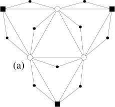
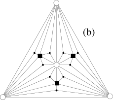
Figure 4: Illustrations of two deterministic scale-free networks: (a) the pseudo-fractal network gonzalez04 , and (b) the Apollonian network hanspriv . Identical symbols label nodes belonging to the same generation $n$ (see text), namely $\bigcirc$ for $n=0$, $\blacksquare$ for $n=1$ and $\bullet$ for $n=2$.

From Fig. 4 and the description above, one easily concludes that for the pseudo-fractal network the outgoing connectivity is fixed at $k=2$, while for Apollonian networks one has $k=3$. Despite both networks have a small number of outgoing connections, they are quite different from the geometrical point of view. In fact, while the pseudo-fractal network has no metric, Apollonian networks are embedded in Euclidean space and fill it densely as $n\to\infty$, being particularly suited for describing geographical situations hanspriv .

As mentioned by Barabási et al barabasi01 , a strong advantage of deterministic networks is that it is often possible to compute analytically their properties, for example the adjacency matrix, whose eigenvalue spectrum characterizes the topology albert02 . A simple way to write the adjacency matrix of the pseudo-fractal network is

$${\cal A}_{n}=\left[\begin{array}[]{cc}{\cal A}_{n-1}&{\cal M}_{n-1}\\ {\cal M}_{n-1}^{T}&\emptyset\end{array}\right]_{L_{n}\times L_{n}}\;,$$ (10)

where $L_{n}$ is given by Eq. (8a), ${\cal M}^{T}$ represents the transpose matrix of ${\cal M}$ and for each generation $n=1,2,\dots$ the matrix ${\cal M}_{n}$ reads

$${\cal M}_{n}=\left[\begin{array}[]{ccc}{\cal M}_{n-1}&{\cal M}_{n-1}&\emptyset\\ \emptyset&\emptyset&{\cal B}_{n-1}\end{array}\right]_{2\cdot 3^{n-1}\times 3^{n}}\;,$$ (11)

with

$${\cal B}_{n-1}=\left[\begin{array}[]{cccc}{\cal A}_{0}&\emptyset&\dots&\emptyset\\ \emptyset&{\cal A}_{0}&\dots&\emptyset\\ \vdots&\vdots&\ddots&\vdots\\ \emptyset&\emptyset&\dots&{\cal A}_{0}\end{array}\right]_{3^{n-1}\times 3^{n-1}}$$ (12)

and whose starting form is

$${\cal M}_{0}={\cal A}_{0}=\left[\begin{array}[]{ccc}0&1&1\\ 1&0&1\\ 1&1&0\end{array}\right]_{3\times 3}\;.$$ (13)

For the Apollonian network, the adjacency matrix is given by the same recurrence of Eq. (10), but this time with

$${\cal A}_{0}=\left[\begin{array}[]{cccc}0&1&1&1\\ 1&0&1&1\\ 1&1&0&1\\ 1&1&1&0\end{array}\right]\;,$$ (14)

and ${\cal M}_{n}$ being a matrix with $(3^{n}+5)/2$ rows and $3^{n}$ columns and having in each column three non-zero elements only.

Figure 5: Typical histogram of the standard mean square-deviation $\hbox{log}_{10}\ \sigma^{2}$ for the pseudo-fractal network as a function of the coupling strength $\varepsilon$. Similar result is obtained for the Apollonian network. Nodes are ruled by the map $f(x)=1-2x^{2}$ and we fixed $\alpha=0$. For the pseudo-fractal network we fixed the number of nodes $L=1095$ ($6$ generations of nodes), while for the Apollonian network $L=1096$ ($6$ generations of nodes). For each coupling strength, the value $N$ indicates the fraction of $500$ initial configurations, and we used transients of $10^{4}$ time steps.

For stability analysis purposes (see Section I), one could derive the Laplacian matrices directly from these adjacency matrices, multiplying the adjacency matrices by $-1$ and adding the appropriate number of connections of each node $i$ along the main diagonal.

As shown in Fig. 5, despite having quite similar structural properties dorogovtsev02 ; hanspriv , the global dynamics of the entirely deterministic scale-free networks shows quite different behavior than the one observed for the Barabási-Albert model in the previous section. Namely, there is no coherence observed for the fully chaotic map for $a=2$. In fact, from Fig. 5 one sees that the standard mean square-deviation never vanishes. Instead, it is characterized by some large value which is almost constant beyond the weak coupling regime ($\varepsilon\gtrsim 0.2$). In the weak coupling regime ($\varepsilon\lesssim 0.2$) the standard mean square-deviation is even larger, since the coupling is not strong enough to compensate the highly chaotic local dynamics ($a=2$). Our simulations have shown that this feature remains valid for any transient up to $10^{6}$ time steps, and it seems to be valid for any value of $a$ for which the quadratic map supports chaotic orbits. One possible physical explanation for this absence of synchronizability is that long range random connections are crucial to improve the ability for synchronization and, due to the deterministic construction of the network, there are no long range connections as in the Barabási-Albert scale-free network. Rigorously speaking, the absence of synchronizability is valid only within the range $0\leq\varepsilon\leq 1$. Of course that, as long as condition (5) holds, there is for sure some range of coupling strengths for which the coherent states are stable. However, since we are working with maps of the interval, we neglect coupling strengths outside the unit interval, otherwise it is not possible to guarantee convergence for all initial configurations.

Figure 6: Histogram of the standard mean square-deviation $\sigma^{2}$ as a function of nonlinearity $a$ and coupling strength $\varepsilon$, for deterministic scale-free networks, namely (a) pseudo-fractal network and (b) Apollonian network. The mean square-deviation is averaged over a sample of $500$ initial configurations and during $100$ time steps, after discarding transients of $10^{4}$ time steps. Here $\alpha=0$ and the base of the logarithm is $10$.

Figure 7: Transitions to coherence in deterministic scale-free networks, when synchronizing the first $g$ generations of nodes out of $\ell$ generations (see text). (a) pseudo-fractal network and (b) Apollonian network. The collective dynamical behavior is quite insensitive to hubs (see text). Insets show that transitions to coherence are of first-order. For each network, we use $\ell=9$ generations of nodes and $a=2$ fixed. The base of the logarithm is $10$.

Figure 8: Inducing transition to coherence by varying the heterogeneity $\alpha$ (see Eq. (1)) in scale-free networks. (a) pseudo-fractal network and (b) Apollonian network. For strong heterogeneity coherence appears beyond a relatively high coupling strength, but it disappears again for very large couplings (see text). For each network, we use $\ell=6$ generations of nodes and fix $a=2$. (c) and (d) show high-resolution plots of $\sigma^{2}$ as a function of $\varepsilon$ for $\alpha=2$, emphasizing the first-order phase transition to coherence. The base of the logarithm is $10$.

We plot the average $\langle\hbox{log}_{10}\ \sigma^{2}\rangle$ as a function of both the nonlinearity $a$ and the coupling strength $\varepsilon$ simultaneously. Figure 6 shows this dependence for the full range of the coupling strength $0\leq\varepsilon\leq 1$ and for nonlinearities above the accumulation point of the first period-doubling cascade of the quadratic map, namely $a\simeq 1.411$. In Fig. 6a we use a pseudo-fractal network, while in Fig. 6b the Apollonian network is considered. In both cases six generations of nodes are taken, yielding a total of $L=1095$ nodes for the pseudo-fractal network and $L=1096$ for the Apollonian network.

As can be seen from these figures, in both cases one has two main regions: (I) a region where the standard mean square-deviation is large and varies smoothly with the parameters and (II) a region where the mean square-deviation is smaller but has larger fluctuations. For the Apollonian network the irregular region is characterized by significantly smaller values for the standard mean square-deviation.

The results observed in the histograms of Fig. 6 are somehow surprising, since irregular variations of the standard mean square-deviation occur for low nonlinearity and high coupling strengths, precisely where one would expect the most regular behavior of the node dynamics. However, this irregularity is just apparent, since $\langle\hbox{log}_{10}\ \sigma^{2}\rangle$ is an average over a sample of initial conditions. Whenever some initial configuration leads to coherence the zero standard deviation decreases this average. Therefore, for $a<1.7$, i.e. in the region of irregular variations of $\sigma^{2}$, coherent solutions are observed. In fact, from the stability condition in Eq. (5) one sees that for periodic maps, the lower boundary of the $\varepsilon$-range is always negative while the upper is positive, yielding always a finite range of coupling strengths where synchronizability is possible. Since for Apollonian networks, the fluctuations occur at small values of the standard deviation, this means that there is probably a larger number of coherent solutions.

Figure 6 indicates that there is a lack of coherent solutions above $a\sim 1.7$. To explain this fact one should notice that both the pseudo-fractal and Apollonian networks have small outgoing connectivities, $k=2$ and $k=3$ respectively. Since one also observes almost no coherent solution for random scale-free networks neither for $k=2$ nor for $k=3$ (see Section II), we believe that the outgoing connectivity $k$ is the main parameter controlling synchronization between oscillators in complex networks. By choosing another deterministic scale-free network with a higher outgoing connectivity, say $k=10$, one might see coherent solutions beyond a coupling threshold value approximately similar to those computed for random scale-free networks (see Fig. 3).

In the remainder of this section we will consider the two deterministic scale-free topologies, and study possible ways of inducing coherent states.

Starting from a total number of $\ell$ generations, one efficient way of inducing coherence is by imposing synchronization among a certain number of $g<\ell$ generations. By generation we mean the set of new nodes appearing simultaneously at a given iteration $n$, during the ‘construction’ of the network. For instance, in the Apollonian network, the first generation has $L_{1}=3$ nodes, the second has $L_{2}-L_{1}=9$ and the $n$th generation has $L_{n}-L_{n-1}=3^{n}$ nodes. In other words, we are interested in the collective effects when the most connected nodes (hubs) are synchronized. We will show that, in fact, hubs play no dominant role for the synchronization of nodes.

Figure 7 shows the standard mean square-deviation as a function of coupling strength for pseudo-fractal (Fig. 7a) and Apollonian networks (Fig. 7b). In each case we choose the fully chaotic map ($a=2$) and impose synchronization among the nodes of the first $g$ generations by setting them to be their mean amplitude at each time-step.

For both networks, one sees from Fig. 7 that the standard mean square-deviation remains large when synchronization is imposed to all $g<\ell-2$ generations. Coherent solutions are only observed for $g=\ell-2$ and $g=\ell-1$, beyond a coupling threshold which is smaller for the latter case. Surprisingly, for $g=\ell-1$ the transition to coherence occurs precisely for the same coupling strength in both networks. This may be due to the fact that, the fraction $L_{g}/L_{\ell}$ of nodes on which one imposes synchronization is approximately the same for both networks. For $g=\ell-2$ the pseudo-fractal network shows coherence only above very high coupling strengths, near $\varepsilon\sim 1$, while for Apollonian networks the threshold is much lower. Although in this case the fraction of nodes on which one imposes synchronization is also similar for both networks, it is much smaller than in the case where $g=\ell-1$. The transition to coherence occurs at different coupling strengths because the number of synchronized nodes is not enough to suppress the effect of the outgoing connectivity. So, since the outgoing connectivity is larger for the Apollonian network, its transition to coherence occurs for weaker coupling strengths. For both networks, one obtains similar results for any higher value $\ell$ of generations since the quotient of the number of nodes between two successive generations $L_{n}/L_{n-1}\to 3$ as $n$ increases.

As a general remark, one observes from Fig. 7 that one needs to synchronize a rather high number of generations to induce coherence. Therefore, it seems that, dynamical collective behavior on scale-free networks is quite insensitive to hubs. As shown in the insets of Fig. 7a and 7b, the transition to coherence is of first-order.

Another way to induce coherence in these two deterministic scale-free networks is, instead of imposing synchronization to the most connected nodes, to strengthen their coupling to the other nodes by taking $\alpha>0$ in Eq. (1). Figure 8 illustrates the transition to coherence by varying the heterogeneity $\alpha$ for the pseudo-fractal (Fig. 8a) and the Apollonian network (Fig. 8b). For both networks, one sees that coherence sets in for $\alpha\gtrsim 1.5$, and only beyond a certain threshold of the coupling strength.

In particular, one observes the remarkable fact that coherence appears only in an intermediate coupling range, i.e. neither to large nor to small values. This is in agreement with previous works pecora97 concerning other systems of coupled chaotic oscillators, where one also observes that synchronized chaos requires that the coupling must be neither too weak nor too strong in order to avoid triggering spatial instabilities strogatz01 . From Figs. 8c and 8d one observes that all these transitions to coherence are of first-order.

For the pseudo-fractal, the upper threshold disappears when the heterogeneity $\alpha$ is further increased. However, for the Apollonian network the upper threshold not only persists but it shifts toward smaller and smaller coupling strengths when $\alpha$ is further increased. As far as we know, this is the first time that one observes such behavior, and it should be related to the geometrical differences between both networks. In other words, since Apollonian is a very particular scale-free network, being the only one, studied so far which is embedded in Euclidean space, this particular feature seems to enable nontrivial synchronization behavior: stronger dominance in the coupling to the most connected nodes destroys coherence.

IV Discussion and conclusions

In this paper we studied fully synchronized solutions for three scale-free network topologies. The main conclusion is the following: in random scale-free networks synchronization of chaotic maps not only depends on the coupling strength but is mainly controlled by the outgoing connectivity $k$, which is a measure of cohesion in the networks. Because of that, one finds coherent solutions in random scale-free networks of fully chaotic logistic maps ($a=2$) with outgoing connectivity $k=8$ and homogeneous coupling, but not in deterministic scale-free networks, since they have rather small effective outgoing connectivity, namely $k=2$ for the pseudo-fractal network and $k=3$ for the Apollonian network.

Therefore, although the exponent $\gamma$ of connection distributions in scale-free networks does not depend on the outgoing connectivity albert02 , we have shown that, in general, synchronization of chaotic maps in such coupling topologies is quite sensitive to it. Moreover, the transition to coherence is of first-order, indicating a similarity with other complex networks strogatz01 . In particular, the threshold values of the coupling strength obey a power-law, Eq. (7), as function of the outgoing connectivity. The exponent of this power-law depends on the nonlinearity $a$ of the chaotic map, being almost constant below $a_{c}\sim 1.7$ and decreasing linearly above it. Interestingly this value of $a_{c}$ is in the vicinity of the bifurcation of the quadratic map where the period-$3$ window appears, and coincides with the appearance of other nontrivial behaviors in coupled map lattices with regular topologies, namely in the velocity distribution of traveling wave solutions lind04b .

The synchronization criterion was based here in the square mean standard deviation following previous studies jost01 . Of course, it could be possible to have numerically a zero standard deviation $\sigma^{2}\sim 10^{-30}$ with a particular oscillator slightly nonsynchronized. However, in such case the deviation of the oscillator amplitude from the rest of the network would be of the order of $10^{-15}$, a majorant of the precision for our criterion. Therefore, we believe that within this numerical precision there are no spurious results. Further investigations could be done, implementing extensions of clustering criteria such as, e.g., that of Pikovsky et al. pikovsky01 .

For deterministic scale-free networks with homogeneous coupling, the same value $a_{c}$ indicates the threshold above which no coherent solutions are observed, independently of the coupling strength. Above $a_{c}$, coherence is observed only for heterogeneous coupling, namely for $\alpha\gtrsim 1.5$. However, for this range of values, we have also shown that coherence is also absent either for very small or for very large coupling strengths, due to spatial instabilities. Another particularly interesting result that still needs to be explained is that, for Apollonian networks, the coupling threshold beyond which coherence disappears gets smaller when the heterogeneity is further increased. This point is not observed for the pseudo-fractal network and may be due to the geometrical differences between both deterministic networks.

As a general property, we have shown that all transitions to coherence are of first-order. Furthermore, all results are robust not only against changes of the initial configurations of node amplitude but also, in random scale-free networks, against changes of the connection network. We also presented preliminary results indicating that in scale-free networks hubs play apparently no fundamental role in the dynamical collective behavior, what remains to be further investigated.

References

- (1) S. Bornholdt and H.G. Schuster (eds.) Handbook of Graphs and Networks (Wiley-VCH, Weinheim, 2003).
- (2) R. Albert and A.-L. Barabási, Rev. Mod. Phys. 74, 47 (2002).
- (3) S.N. Dorogovtsev and J.F.F. Mendes, Adv. Phys. 51, 1079 (2002).
- (4) R. Meucci, R. McAllister, and R. Roy, Phys. Rev. E 66, 026216 (2002).
- (5) J.H. Snoeijer, T.J.H. Vlugt, M. van Hecke, and W. van Saarloos, Phys. Rev. Lett. 92, 054302 (2004).
- (6) M. Otto, J.-P. Bouchaud, P. Claudin, and J.E.S. Socolar, Phys. Rev. E 67, 031302 (2003).
- (7) C. Texier and G. Montambaux, Phys. Rev. Lett. 92, 186801 (2004).
- (8) H. Tanaka, J. Meunier, and D. Bonn, Phys. Rev. E 69, 031404 (2004).
- (9) D.P. Almond and C.R. Bowen, Phys. Rev. Lett. 92, 157601 (2004).
- (10) M. Small and C.K. Tse, Phys. Rev. E 66, 066701 (2002).
- (11) I. Stewart, Nature 427, 601 (2004).
- (12) Y. Moreno, M. Nekovee and A. Vespignani, Phys. Rev. E 69, 055101(R) (2004).
- (13) Z. Dezso and A.L. Barabási, Phys. Rev. E 65, 055103 (2002).
- (14) M. Compiani, E. Capriotti, and R. Casadio, Phys. Rev. E 69, 051905 (2004).
- (15) L. Zhaoping, A. Lewis and S. Scarpetta, Phys. Rev. Lett. 92, 198106 (2004).
- (16) P.G. Lind, J. Corte-Real and J.A.C. Gallas, Phys. Rev. E 69, 026209 (2004).
- (17) S.H. Strogatz, Physica D 143, 1 (2000).
- (18) L.M. Pecora, T.L. Carroll, G.A. Johnson, D.J. Mar and J.F. Heagy, Chaos 7, 520 (1997).
- (19) C. Anteneodo, A.M. Batista and R.L. Viana, Phys. Lett. A 326, 227-233 (2004).
- (20) P. Erdös and A. Rényi, Publ. Math. Debrecen 6, 290 (1959).
- (21) S.H. Strogatz, Nature 410, 268 (2001).
- (22) D.J. Watts and S.H. Strogatz, Nature 393, 440 (1998).
- (23) A.-L. Barabási and R. Albert, Science 286, 509-512 (1999).
- (24) S.C. Manrubia and A.S. Mikhailov, Phy. Rev. E 60, 1579 (1999).
- (25) J. Jost and M.P. Joy, Phys. Rev. E 65, 016201 (2001).
- (26) T. Nishikawa, A.E. Motter, Y.-C. Lai, and F.C. Hoppensteadt, Phys. Rev. Lett. 91, 014101 (2003).
- (27) M. Barahona and L.M. Pecora, Phys. Rev. Lett. 89, 054101 (2002).
- (28) L.F. Lago-Fernández, R. Huerta, F. Corbacho and J.A. Siguenza, Phys. Rev. Lett. 84, 2758 (2000).
- (29) H. Hong, B.J. Kim, M.Y. Choi, and H. Park, Phys. Rev. E 69, 067105 (2004).
- (30) F.M. Atay, J. Jost and A. Wende, Phys. Rev. Lett. 92, 144101 (2004).
- (31) X.F. Wang and G. Chen, IEEE Trans. Circ. Sys. I 49, 54 (2002).
- (32) L.M. Pecora and T.L. Carroll, Phys. Rev. Lett. 80, 2109 (1998).
- (33) K.S. Fink, G. Johnson, T. Carroll, D. Mar and L. Pecora, Phys. Rev. E 61, 5080 (2000).
- (34) S.C. Manrubia, A.S. Mikhailov and D.H. Zanette Emergence of Dynamical Order Synchronization Phenomena in Complex Systems, vol. 2 (World Scientific, Singapore, 2004).
- (35) A.E. Motter, C. Zhou and J. Kurths, cond-mat/0406207 (2004).
- (36) P.G. Lind, J.A.C. Gallas and H. Herrmann, manuscript in preparation (2004).
- (37) A.-L. Barabási, E. Ravasz, and T. Vicsek Physica A 299, 559 (2001).
- (38) S.N. Dorogovtsev, A.V. Goltsev, and J.F.F. Mendes, Phys. Rev. E 65, 066122 (2002).
- (39) J.S. Andrade Jr., H.J. Herrmann, R.F.S. Andrade, and L. da Silva, “Apollonian networks”, cond-mat/0406295 (2004).
- (40) K. Iguchi and H. Yamada, “Exactly solvable scale-free network model”, cond-mat/0405662, 2004.
- (41) M.C. González, A.O. Sousa, and H.J. Herrmann, Int. J. Mod. Phys. C 15, 45 (2004).
- (42) P.G. Lind, J. Corte-Real and J.A.C. Gallas, Phys. Rev. E 69, 066206 (2004).
- (43) A. Pikovsky, O. Popovych and Yu. Maistrenko, Phys. Rev. Lett. 87, 044102 (2001).