Energy landscape of a simple model for strong liquids

Abstract

We calculate the statistical properties of the energy landscape of a minimal model for strong network-forming liquids. Dynamic and thermodynamic properties of this model can be computed with arbitrary precision even at low temperatures. A degenerate disordered ground state and logarithmic statistics for the local minima energy distribution are the landscape signatures of strong liquid behavior. Differences from fragile liquid properties are attributed to the presence of a discrete energy scale, provided by the particle bonds, and to the intrinsic degeneracy of topologically disordered networks.

In recent years, the study of the statistical properties of the potential energy surface or landscape (PES) wales ; debenedetti01 ; angell95 sampled by liquids in supercooled states has received considerable attention, in the attempt to quantify the thermodynamic properties of supercooled liquids and glasses stillinger_pes ; sastry01 ; st ; press . The PES is analyzed to estimate the number and energy distribution $\Omega(E)$ of the local minima and the volume in configuration space sampled in vibrational motions around each local minimum.

According to Angell’s classification fragdef , a liquid is named ”fragile” if the temperature dependence of its transport coefficients shows large deviations from Arrhenius behavior. If no deviations are observed, the liquid is named ”strong”. For the case of fragile liquids — in the region of energies sampled during low temperature $T$ equilibrium simulations with state of the art numerical resources — $\Omega(E)$ is well described by a Gaussian distribution sastry01 ; heuer00 ; press . The validity of Gaussian statistics in regions of the PES with energy lower than those accessible in simulations, would suggest the existence of a finite Kauzmann temperature $T_{K}$, where the configurational entropy $S_{conf}$ vanishes, and via the Adam-Gibbs relation adam65 ; wolynes , a divergence of the characteristic relaxation time at $T_{K}$. The quantification of the statistical properties of the PES for models of strong liquids is still under debate voivod01 ; newheuer . It has been shown that, on lowering $T$, deviations from Gaussian statistics take place. The configurational entropy does not seem to extrapolate to zero at a finite $T$, but the long equilibration times and the unknown value of the ground state energy prevent an unambiguous determination of the ground state degeneracy. A recent work of Heuer and coworkers newheuer suggests that the breakdown of Gaussian statistics originates from the emergence of a natural cut-off in $\Omega(E)$, related to the formation of a fully connected network of bonds.

In this Letter, we report a study aiming to clarify the statistical properties of the PES for a strong liquid, to provide a useful framework for interpreting results of realistic models, and to shed light on the differences between fragile and strong liquids. We quantify the landscape properties for a simple model, similar in spirit to one previously introduced by Speedy and Debenedetti speedymaxval . We show that, with appropriate numerical techniques, both the dynamics and thermodynamic properties of this model can be computed with high accuracy and that no extrapolations are required to determine the low $T$ behavior. The strong liquid behavior is associated with the presence of two ingredients, which are characteristic of all network-forming liquids: a degenerate ground state and a discrete distribution of energies above the ground state, generated by the bond energy scale.

We investigate a maximum valency model: a square well model of width $\Delta$ with a constraint on the maximum number of interacting particles. The interaction between two particles $i,j$ that each have less than $N_{max}$ bonds to other particles, or between two particles already bonded to each other, is given by a square-well potential,

$$V_{ij}(r)=\begin{cases}~{}~{}\infty~{}~{}~{}~{}~{}~{}~{}\hskip 2.27621ptr<\sigma\\ -u_{0}~{}~{}~{}~{}~{}~{}~{}\sigma<r<\Delta\\ ~{}~{}~{}0~{}~{}~{}~{}~{}~{}~{}~{}r>\sigma+\Delta.\end{cases}$$ (1)

When $i$ and/or $j$ are already bonded to $N_{max}$ neighbors, then $V_{ij}(r)$ is simply a hard sphere (HS) interaction,

$$V_{ij}(r)=\begin{cases}~{}~{}\infty~{}~{}~{}~{}~{}~{}~{}~{}r<\sigma\\ ~{}~{}~{}0~{}~{}~{}~{}~{}~{}~{}~{}\hskip 2.27621ptr>\sigma.\end{cases}$$ (2)

The maximum number of bonds per particle is controlled by tuning $N_{max}$. This model is particularly suited for theoretical and numerical studies. First of all, along an isochore, the system changes from a HS system (when $k_{B}T\gg u_{0}$, $k_{B}$ is the Boltzmann constant) to a simple model for network-forming liquids (when $k_{B}T<u_{0}$) with coordination $N_{max}$ and no angular constraints noangcons . Second, the ground state energy for a system of $N$ particles is known, being the energy of a fully connected network ($-u_{0}NN_{max}/2$). Third, as $V(r)$ is simply a square well model, the local minima of the PES coincide with the bonding patterns of the system. Consequently, moving between minima takes place via breaking and reforming of bonds. Fourth, the volume in configuration space of each of these bonding patterns can be calculated with no approximation, as discussed in the following. In the PES language, it means that the basin free energy stillinger_pes can be calculated exactly. Finally, since the energy levels of the system are discrete by construction, the number of bonding patterns with $M<<NN_{max}/2$ broken bonds can be calculated by combinatorial factors. Exploiting these properties allows us to quantify precisely the statistical properties of the PES of this model.

We perform Monte Carlo (MC) and event driven molecular dynamics simulations by using $\Delta/(\sigma+\Delta)=0.03$, $u_{0}=1$, $\sigma=1$ and $N_{max}=4$. Entropy, $S$, is measured in units of $k_{B}$. Setting $k_{B}=1$, energy $E$ and temperature $T$ are measured in units of $u_{0}$. We study a system of $N=10^{4}$ particles of equal mass $m=1$, implementing periodic boundary conditions, at a fixed packing fraction $\phi=0.30$ packfrac from temperature $T=100$ (where the HS limit is recovered) down to $T=0.04$, where an almost fully connected network of bonds is obtained mapping . No evidence of phase separation is observed zaccar . Fig. 1a shows the $T$ dependence of the potential energy per particle $E$ as a function of $1/T$. For a Gaussian PES sastry01 ; REM , $E$ should be linear in $1/T$. Deviations from the $1/T$ law are clearly seen at low $T$, when the energy approaches the ground state energy $E_{gs}=-2$, with a striking similarity with the $T$ dependence of the energy of the sampled minima evaluated in landscape analyses of atomistic models for silica voivod01 ; newheuer . The approach to $E_{gs}$ is well described by $E-E_{gs}\sim e^{-\frac{1}{2T}}$, providing an unambiguous way of calculating all thermodynamic properties down to $T=0$.

Next we provide evidence that the present model is a simple and satisfactory one for strong glass-forming liquids, by showing several features that are commonly observed in real systems. Fig. 1b shows the $T$ dependence of $\eta$ and $D$ visc . Both quantities display Arrhenius behavior at low $T$, as expected for strong liquids, with an activation energy controlled by the bond energy. The product $\frac{D\eta}{T}\approx\frac{1}{3\pi\sigma}$, as expected from the Stokes-Einstein relation. We also evaluate the exponent $\beta$ of the stretched exponential function that describes the long time decay of density autocorrelation functions, finding values $\beta>0.85$ for all the wavevectors. Such a large $\beta$ value is in agreement with the experimentally observed direct correlation between $\beta$ and strong behavior bohmer . Finally, since at the investigated low $T$ the potential energy has already approached the ground state value (Fig. 1a), no signifficant drop in the specific heat will take place at the glass transition temperature. This feature is often found in strong liquids martinez ; richet .

Next we evaluate the statistical properties of the PES. In the landscape approach, configuration space is partitioned into basins around the local minima of the PES. For the present model, different local minima can be unambiguously identified as different bonding patterns and the energy of the minimum coincides with the potential energy of the configuration, i.e. with the number of bonds. The partition function can be written as a sum over all bonding patterns. At low $T$, it is convenient to write the sum over the number of $M$ broken bonds, associating with each energy level $E$ the number of distinct network configurations with $M\equiv(E-E_{gs})N$ broken bonds (the degeneracy of the energy level) times the volume in configuration space that can be sampled by the network without breaking or forming any bond (i.e. preserving the bonding pattern). The logarithm of the number of distinct networks with the same number of bonds defines $S_{conf}(E)$, while the logarithm of the sampled volume defines the basin vibrational entropy $S_{vib}$. The sum $S_{conf}+S_{vib}$ defines the total entropy of the model.

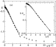
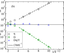
Figure 1: Temperature dependence of the potential energy per particle $E$ (top) and of $\eta$ (in units of $(mu_{0})^{1/2}/\sigma^{2}$), $D$ (in units of $\sigma(u_{0}/m)^{1/2}$), and the product $D\eta/T$ (bottom). $D$ is calculated from the long time limit of $\delta r^{2}(t)/6t$, with $\delta r^{2}(t)$ the mean squared displacement, and $\eta$ as explained in alder . In the top panel, the dashed line shows the $1/T$ behavior expected for a Gaussian landscape sastry01 ; REM . The inset shows the same data in a semi-log representation to highlight the validity of the low-T behavior $\ln[E-E_{gs}]=\ln[2.56]-\frac{1}{2T}$ indicated by the continuous line (see text). In the bottom panel the dashed lines are the best-fit Arrhenius behavior for $\eta$ and $D$. The continuous line corresponds to the expected value from the Stokes-Einstein relation (see text).

In the present model, $S_{vib}$ can be calculated without approximation by thermodynamic integration from a reference Einstein crystal frenkel . In this technique, a series of MC simulations are performed adding to the original Hamiltonian $H_{0}$ a harmonic perturbation $H_{E}(\vec{r}^{N};\lambda)=\lambda\sum_{i=1}^{N}(\vec{r}_{i}-\vec{r}_{i}^{0})^{2}$, where $(\vec{r}_{1}^{0},...,\vec{r}_{N}^{0})$ is a typical configuration of energy $E$ whose basin free energy needs to be evaluated, and the parameter $\lambda$ is the elastic constant of the harmonic perturbation. The system described by the Hamiltonian $H(\vec{r}^{N};\lambda)=H_{0}(\vec{r}^{N})+H_{E}(\vec{r}^{N};\lambda)$ is then simulated at fixed $T$ and $V$ with a MC technique, rejecting all moves altering the bonding pattern. We study several values of $\lambda$ running from $\lambda=0$ up to a value $\lambda_{max}$, whereupon the behavior of a system composed of 3$N$ independent harmonic springs of elastic constant $\lambda_{max}$ is recovered. In this limit, the free energy is known analytically. The vibrational free energy $f_{vib}$ ($\lambda=0$) of the basin to which $\vec{r}^{0}$ belongs is given by

$$f_{vib}(T)=F_{H_{E}}(T;\lambda_{max})$$

$$-\int_{-\infty}^{ln[\lambda_{max}]}\lambda\langle\sum_{i=1}^{N}(\vec{r}_{i}-\vec{r}_{i}^{0})^{2}\rangle_{\lambda}dln[\lambda],$$ (3)

where $\sum_{i}(\vec{r}_{i}-\vec{r}_{i}^{0})^{2}$ is the sum of the square displacements of all particles at a fixed value of $\lambda$, brackets denote ensemble average, and $F_{H_{E}}(T;\lambda_{max})$ is the free energy of the 3$N$ Einstein oscillators. Fig. 2 shows the $\lambda$ dependence of $\lambda\langle\sum_{i}(\vec{r}_{i}-\vec{r}_{i}^{0})^{2}\rangle_{\lambda}/N$ for one specific state point. At large $\lambda$ values, the mean square displacement per particle approaches the theoretically expected limit $\frac{3}{2}\frac{k_{B}T}{\lambda}$. It must be noted that in the present model, since no energy changes are involved in sampling the configuration space volume at fixed bonding pattern, for each specific basin the basin free energy is purely entropic.

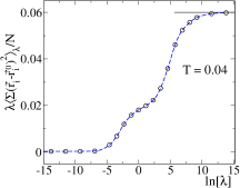
Figure 2: Mean squared displacement per particle times $\lambda$ as a function of $ln[\lambda]$ for a typical basin explored at $T=0.04$. The continuous line shows the harmonic behavior $\frac{3}{2}k_{B}T$.

Repeating the thermodynamic integration procedure for several different equilibrium configurations at different $T$, $S_{vib}(E)$ can be precisely calculated. Fig. 3a shows that the excess quantity, $S_{vib}^{ex}(E)$, over the ideal gas contribution, depends linearly on the basin depth $E$, a feature shared with previously investigated models for supercooled liquids sastry01 ; press ; wales . $S_{vib}^{ex}(E)$ is well represented by the best-fit function:

$$S^{ex}_{vib}=-8.8+4.27(E-E_{gs}).$$ (4)

Complementing these data with the calculation of the excess total entropy over the ideal gas contribution, $S_{tot}^{ex}$, by integration of the $T$ dependence of the specific heat over $T$ from the known HS high $T$ reference state frenkel , allows us to evaluate $S_{conf}\equiv S_{tot}^{ex}-S_{vib}^{ex}$. Fig.3b shows that, close to the ground state, the $E$ dependence of $S_{conf}$ is well described by a logarithmic combinatorial function:

$$S_{conf}(E)=S_{conf}(E_{gs})$$

$$-2(E-E_{gs})\ln[2(E-E_{gs})]+(E-E_{gs}).$$ (5)

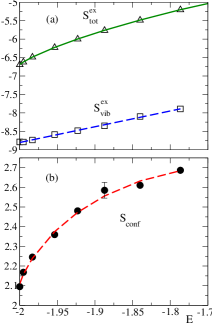
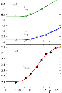
Figure 3: Energy $E$ [panels (a) and (b)] and $T$ [panels (c) and (d)] dependence of $S_{tot}^{ex}$, $S_{vib}^{ex}$ and $S_{conf}$. A typical error bar is shown in panel (b). Dashed lines for $S^{ex}_{conf}(E)$ and $S^{ex}_{vib}(E)$ are fits to Eqs.4-5 (see text). The continuous line for $S_{tot}^{ex}$ is the result of summing the obtained fit functions. The continuous lines for $S_{tot}^{ex}(T)$, $S_{vib}^{ex}(T)$ and $S_{conf}(T)$ are calculated from the $T$ dependence of $E$ (see text).

The logarithmic term results from the number of distinct ways $(E-E_{gs})N$ bonds can be broken among $N$ particles. A one-parameter fit (see Fig. 3b) suggests $S_{conf}(E_{gs})\approx 2.1$ uppersconf . Eqs. 4-5 fully define the statistical properties of the PES. All thermodynamic functions can be evaluated from them. Indeed, solving $d(S_{conf}+S^{ex}_{vib})/dE=1/T$, the $T$ dependence of $E$ is found to be $E(T)-E_{gs}=2.56e^{-\frac{1}{2T}}$, providing the continuous line in the inset of Fig. 1a, and parametrically, the continuous lines for $S^{ex}(T),S^{ex}_{vib}(T)$ and $S_{conf}(T)$, compared with the numerical estimates in Figs. 3c-3d.

According to the picture emerging from this study, strong liquid behavior is connected to the existence of an energy scale (provided by the bond energy) which is discrete and dominant as compared to the energetic contributions coming from non-bonded next-nearest neighbor interactions angellbond . It is also intimately connected to the existence of a significantly degenerate ground state, favoring the formation of highly bonded states which can still entropically rearrange to form different bonding patterns with the same energy schwabl . The presence of the bond energy scale impure also determines a distribution of energy levels above the disordered ground state which are logarithmically spaced. These results help rationalize previous landscape analysis of realistic models of network-forming liquids voivod01 and the recent observation by Heuer and coworkers that the breakdown of Gaussian landscape statistics is associated with the formation of a fully connected defect-free network newheuer . While in realistic models the ground state energy is not known, and the very long equilibration times needed prevent an unambiguous determination of the ground state degeneracy, both these quantities can be calculated for the present model.

In this model, the discrete energy states provide a truly degenerate ground state. In real systems, small differences in energy exist, e.g. resulting from second neighbor interactions, between configurations that in our model would correspond to the same energy state. Hence, in real systems the “ground state” energy is smeared out, singling out a unique lowest energy state. Consequently, for $k_{B}T$ values smaller than this spread in energy, $S_{conf}$ approaches zero. Therefore, our classical model is strictly applicable at temperatures where quantum effects are negligible quantum , and for values of $k_{B}T$ much larger than the spread in energy of the ground state.

The simplicity of the model and the possibility of calculating accurately the relevant thermodynamic properties at all $T$ makes this model a relevant candidate for deepening our understanding of the differences between strong and fragile liquids. Results reported here suggest that strong and fragile liquids are characterized by significant differences in their PES properties. In a simplified picture, a non-degenerate disordered ground state and Gaussian statistics characterize fragile liquids, while a degenerate disordered ground state and logarithmic statistics are associated with strong liquids. The origin of this difference is traced to the presence of a discrete energy scale, provided by particle bonds, and to the intrinsic degeneracy of topologically disordered networks.

We acknowledge support from MIUR-COFIN, MIUR-FIRB, DIPC-Spain, NSF and NSERC-Canada.

References

- (1) D. Wales, Energy Landscapes, Cambridge University Press, Cambridge (2004).
- (2) P. G. Debenedetti and F. H. Stillinger, Nature (London) 410, 259 (2001).
- (3) C. A. Angell, Science 267, 1924 (1995).
- (4) F. H. Stillinger and T. A. Weber, Phys. Rev. A 25, 978 (1982); Science 225, 983 (1984); F. H. Stillinger, ibid. 267, 1935 (1995); F. Sciortino, J. Stat. Mech., P05015, (2005).
- (5) S. Sastry, Nature (London) 409, 164 (2001).
- (6) F. Sciortino et al., Phys. Rev. Lett. 83, 3214 (1999).
- (7) E. La Nave et al., Phys. Rev. Lett. 88, 225701 (2002).
- (8) C. A. Angell, J. Non-Cryst. Solids 73, 1 (1985).
- (9) A. Heuer and S. Buchner, J. Phys.: Condens. Matter 12, 6535 (2000).
- (10) G. Adam and J. H. Gibbs, J. Chem. Phys. 43, 139 (1965).
- (11) X. Xia and P. G. Wolynes, Phys. Rev. Lett. 86, 5526 (2001).
- (12) I. Saika-Voivod et al., Nature (London) 412, 514 (2001).
- (13) A. Saksaengwijit et al., Phys. Rev. Lett. 93, 235701 (2004).
- (14) R. J. Speedy and P. G. Debenedetti, Mol. Phys. 81, 237 (1994); ibid. 86, 1375 (1995); 88, 1293 (1996).
- (15) In Ref.speedymaxval an angular constraint is imposed by avoiding three particles bonding loops.
- (16) Note that a diamond structure of touching hard spheres has , a value compatible with the one we study here. The diamond structure is characteristic of tetrahedral network forming strong liquids like water and silica.
- (17) In the effort to capture the basic ingredients of a strong liquid, angular correlations are completely neglected. Still, the investigated low -regime qualitatively corresponds to typical experimental values. From SiO2 and GeO2 viscosity data above the glass transition temperature richet ; sipp , we estimate Arrhenius activation energies (SiO2) K and (GeO2) K. Assuming the investigated -range in our simulations roughly corresponds to K for SiO2 and K for GeO2, values in the experimental accesible -range richet ; sipp .
- (18) P. Richet, Geochim. Cosmochim. Acta 48, 471 (1984).
- (19) A. Sipp et al., J. Non-Cryst. Sol. 288, 166 (2001).
- (20) E. Zaccarelli et al., Phys. Rev. Lett. 94, 218301 (2005).
- (21) B. J. Alder et al., J. Chem. Phys. 53, 3813 (1970).
- (22) B. Derrida, Phys. Rev. B 24, 2613 (1981).
- (23) Note that in simulations, it is today possible to follow changes in dynamic properties covering up to six orders of magnitude, to be compared to changes in experimental quantities covering about 12 decades.
- (24) R. Böhmer et al., J. Chem. Phys. 99, 4201 (1993).
- (25) L. M. Martinez and C. A. Angell, Nature 410, 663 (2001).
- (26) D. Frenkel and B. Smit, Understanding Molecular Simulation, Academic Press, San Diego (1996).
- (27) The value found here should be considered an upper bound value for tetrahedral networks speedymaxval ; sceats , due to the absence of angular constraints in the bonding geometry.
- (28) M. G. Sceats et al., J. Chem. Phys. 70, 3927 (1979); R. L. C. Vink and G. T. Barkema, Phys. Rev. B 67, 245201 (2003); N. Rivier and F. Wooten, MATCH Commun. Math. Comput. Chem 48, 145 (2003).
- (29) C. A. Angell and K. Rao, J. Chem. Phys. 57, 470 (1972).
- (30) Note that the presence of a residual value of at is not in conflict with the Third Law of Thermodynamics, see, e.g., F. Schwabl, Statistical Mechanics, Springer-Verlag, Berlin Heidelberg (2000).
- (31) Impure network-forming liquids as mixed alkali silicates richet ; bohmer show deviations from strong behavior. Such deviations could originate from the interplay between different bond energies, strongly smearing out the discrete energy scale.
- (32) In a first approximation, quantum effects take place below the temperature where the de Broglie wavelenght becomes comparable to nearest neighbour distances.