Central peak in the pseudogap of high Tc superconductors
Abstract
We study the effect of antiferromagnetic (AF) correlations in the three-band Emery model, with respect to the experimental situation in weakly underdoped and optimally doped BSCCO. In the vicinity of the vH singularity of the conduction band there appears a central peak in the middle of a pseudogap, which is in an antiadiabatic regime, insensitive to the time scale of the mechanism responsible for the pseudogap. We find a quantum low-temperature regime corresponding to experiment, in which the pseudogap is created by zero-point motion of the magnons, as opposed to the usual semiclassical derivation, where it is due to a divergence of the magnon occupation number. Detailed analysis of the spectral functions along the – line show significant agreement with experiment, both qualitative and, in the principal scales, quantitative. The observed slight approaching-then-receding of both the wide and narrow peaks with respect to the Fermi energy is also reproduced. We conclude that optimally doped BSCCO has a well-developed pseudogap of the order of 1000 K. This is only masked by the narrow antiadiabatic peak, which provides a small energy scale, unrelated to the AF scale, and primarily controlled by the position of the chemical potential.
I Introduction
The Fermi surface phenomena in the high-Tc cuprates, and especially BSCCO, have been extensively investigated, and a broad consensus has developed concerning their main features. The Fermi surface is large and hole-like, with a simple topology of a rounded square, or barrel, centered around the M-point Fretwell et al. (2000). Single-particle phenomenology is routinely invoked on the ARPES spectra, thus the ‘self-energy’ and ‘damping’ are often extracted from the main peak as if it were a coherent, weakly perturbed quasiparticle Valla et al. (1999). However, in the underdoped regime and below a temperature scale T∗, the metallic state is surfeit with low-energy correlations, about whose relevance for either the pseudogap, or the superconducting mechanism itself, there is no general agreement at present. Various experimental observations at low energy have been interpreted in terms of stripes Kivelson et al. (2003), paramagnons Sadovskii (2001), phonons Lanzara et al. (2001), and superconducting fluctuations above Tc Ong et al. (2004). All these correlations are at present the object of intense scrutiny, mainly with a view to ascertaining whether they enhance or suppress superconductivity.
Theoretical understanding of the measured electronic spectral functions of high-Tc superconductors has received significant attention in the context of these efforts Shen et al. (1995); Kim et al. (1998); Schabel et al. (1998); Fedorov et al. (1999); Feng et al. (2001); Kaminski et al. (2001); Mesot et al. (2001); Matsui et al. (2003); Campuzano et al. (2004, to appear). Physically, conduction occurs in the copper oxide planes, so the most important electronic states are directly accessible to surface probes such as ARPES. This naturally allows for a concentration of theoretical effort, especially because the observed spectra offer some outstanding puzzles of their own. Such a long-standing issue is the appearance of the pseudogap Randeria (1998), observed near the vH points for underdoped systems, and its connection with the AF gap at lower doping on the one hand, and with the superconducting (SC) gap at lower temperature, on the other. Experimentally, the pseudogap is clearly connected with a correlation Campuzano et al. (2004, to appear), and the most natural candidate for its origin are antiferromagnetic fluctuations above their transition point Sadovskii (2001).
The present work attempts to connect several aspects of the low-energy phenomenology of the cuprates in the hope of realistically constraining the eventual theory of the optimally doped and weakly underdoped state. We adopt an effective weak-coupling framework, and concentrate on aspects least sensitive to model details. Our most important observation is that the pseudogap does not really disappear at optimal doping, but is instead rather inefficient at suppressing part of the spectral strength around the vH points. The unsuppressed strength appears at the Fermi level as an ‘antiadiabatic’ central peak in the middle of a still fairly wide and deep pseudogap. It is the latter ‘high-energy pseudogap’ which indicates the underlying physical scale, while the ‘leading edge’ scale, associated with the central peak, turns out to be incidental to the dynamics. It is primarily controlled by doping. This interpretation does not even depend on the pseudogap being due to antiferromagnetism as such, but only on the fact that the dominant perturbing correlation occurs around the wavevector . It is however different than interpreting the high-energy ‘hump’ in terms of bilayer splitting Feng et al. (2001); Chuang et al. (2001); Kordyuk et al. (2002).
We do not enter here the important question why the magnetic correlations undergo an essential change at Tc. Our main aim is to show that when their observed low-temperature behavior is introduced phenomenologically in the calculation of the single-electron propagator, the resulting antiadiabatic peak and pseudogap behave consistently with the main features of the ‘peak-dip-hump’ structure, found in experiments on superconducting optimally doped BSCCO. In this way our calculation refers to the superconducting state. We only omit the direct effect of superconductivity on the single electron propagation, namely the appearance of a superconducting gap. This is justified by the fact that the SC gap scale in ARPES is an order of magnitude below the AF scale, manifested by the high-energy ‘hump.’ In order to reproduce typical normal-state ARPES profiles, which do not show a narrow low-energy peak, we only need to overdamp the paramagnons. Our work provides a connection between the observed simultaneous appearances of a magnetic resonance and of a narrow low-energy peak in the ARPES profile, as the temperature drops below Tc.
Like some other authors Vilk (1997); Friedel and Kohmoto (2002); Eschrig and Norman (2003), here we use an effective weak-coupling (single-band) approach to describe the effect of antiferromagnetic correlations on the single-electron propagation. Given that is large in the high-Tc superconductors, our starting point is the strong coupling limit, and we use the present calculation to develop a phenomenological framework in which the correct physical regime can be identified for the effective weak-coupling approach. Section II is thus devoted to placing the present work in this wider theoretical context. Section III describes the model results. A comparison with experiment is found in Section IV. Finally, Section V is a recapitulation and discussion.
II The electron self-energy and the central peak
II.1 Separation of charge and spin channels
We enter a brief theoretical discussion now on the validity of the weak-coupling single-band approach, with a large hole-like Fermi surface, when is large. This is the essential input in our calculation, important for its comparison with the -dependencies measured by ARPES.
Recently a considerable improvement in understanding the band dispersion measured by ARPES in the high-Tc superconductors near optimal doping has been achieved by considering the extended Emery model Emery (1987) in the limit of large interactions on the Cu-site. The original Emery model of the CuO2 plane is extended by taking into account the direct O-O hopping in addition to the original Cu-O hopping and the difference of the O and Cu site energies Mrkonjić and Barišić (2003a).
In the limit of interest this means that the ‘broad’ oxygen band is weakly hybridized with the Cu level. The Emery model then resembles the Anderson lattice model which includes the accurate symmetry of the electron (hole) propagation in the CuO2 lattice, either along the O-O axis () or along the Cu-O axis (). Notably, the limit , although probably too extreme for physical purposes, corresponds to the Falicov-Kimball model Falicov and Kimball (1969), also sometimes invoked in the context of high-Tc superconductors Gor’kov and Sokol (1989); Sunko and Barišić (1996); Sunko (2000); Freericks and Devereaux (2001); Sunko (2005).
The large limit of the Emery model Emery (1987) extended by was treated in the homogenous mean field approximation Mrkonjić and Barišić (2003a) applied to the slave-boson representation of the Emery model. The usual objection that the mean-field slave boson (MFSB) approximation breaks the local gauge invariance required by the slave-boson theory was met Mrkonjić and Barišić (2003b) by emphasizing that the static mean field merely represents the slow component of the slave boson field. This latter, allowed by local gauge invariance, only appears as static when particular physical properties are calculated, most notably the physical electron band dispersion. Thus the physical dispersion can be represented by the usual non-interacting three-band dispersion, but with strongly renormalized tight-binding parameters and instead of and , while remains unaffected by the copper on-site repulsion. Most importantly, in this way the observed regime naturally replaces the regime , inferred from chemical valency analysis and high-energy spectroscopy data. The formula for the antibonding electron band is then
| (1) |
where
with and . It is obvious from Eq. (1) that the effective near neighbor hoppings and enter the dispersion non-linearly. This is in contrast to those one-band approaches which include hoppings to unphysically Mrkonjić and Barišić (2004) distant neighbors, but as independent parameters. (Noteworthily, LDA calculations Andersenn et al. (1995) show directly that when such long-range hoppings are induced by reduction of multiband to single-band models, the effective parameters depend non-linearly on the near-neighbor ones, as in our case.) We use the single band (1) from the three-band model with this distinction in mind.
Actually, after taking into account the fast harmonic slave-boson fluctuations around the mean-field saddle point, the MFSB band (1) decomposes into the narrow resonant band with dispersion and a spectral density , which accomodates approximately holes (doping ) on the O-site and one hole localized in the localized state on the Cu-site at the energy , deep below Mrkonjić and Barišić (2003a, b). The observed structure of the resonant band in LSCO is well described Mrkonjić and Barišić (2003a) by the regime and evolves with doping according to MFSB predictions.
Once these renormalizations are taken into account, the remaining low-energy analysis concerns only the resonant band containing the Fermi level. In the above slave-boson calculations the spins of the localized holes on the Cu sites are taken as paramagnetic. This is justified for large enough dopings , when the band-width of the resonant band exceeds the magnetic and/or superconducting energy scales, whereas for models of - type may be more appropriate. Indeed, for optimal dopings the bandwidth is of the order of 1 eV, whereas the magnetic and/or superconducting effects occur on scales lower by at least an order of magnitude. This approach is in principle well suited to take magnetic energies into account as a perturbation of the main energy scales associated with the resonant band. While the formation of the resonant band is associated in the first place with the slow component in the motion of the slave boson, its fast component is alone responsible for the weak magnetic couplings. Several calculations of this type were carried out before for strongly interacting electron systems. In particular, for the Emery model with large , the residual effective couplings were derived explicitly Tutiš (1994). The extension of these ideas to finite , in particular to , with a clear distinction between slow and fast components of the slave-boson field is currently under way. These residual couplings can be treated, for example, by the perturbational 2D parquet theory. At the latter was shown Dzyaloshinskii and Yakovenko (1988) to lead to ladder-like results (‘fast parquet’) in most of the space of coupling parameters, and to the marginal Fermi liquid only under very special conditions. Here we consider this ladder-like regime appropriate for calculating the electron self-energy from Fig. 1, where the wavy line represents the spin susceptibility , and the triangular vertex corrections are neglected.

To summarize, for large there is a natural separation of the slave-boson fluctuations into fast and slow components. The latter appear static when calculating the effective dispersion of the electrons, so in fact our mean-field slave-boson renormalization of the electronic band parameters corresponds to taking this slow component into account in the charge channel Mrkonjić and Barišić (2003b). This explains why the Fermi surface is large and hole-like. The fast component in the spin channel is the paramagnon perturbation of the large, hole-like Fermi surface. In the following, we concentrate entirely on the latter, neglecting triangular vertex corrections in Fig. 1.
II.2 Electron spectral density
Following the ideas expressed above, the fermion line in Fig. 1 is taken to represent hole propagation in the absence of magnetic couplings. In this approach the electron Green’s function appearing in Fig. 1 is free. It has been observed Vilk and Tremblay (1997); Yanase (2004) that corrections from self-consistency tend to cancel with vertex corrections in the absence of Migdal’s theorem, so it appears generally more reliable to take neither into account than only one. Thus the retarded Green‘s function is just
| (2) |
with from Eq. (1), and the spectral density of the resonant band. Based on the above MFSB considerations, we expect a significant -dependence in this quantity along the Fermi surface, once the strong on-site repulsion is explicitly taken into account. In the present work, we concentrate entirely on the vicinity of the vH point, so will eventually be absorbed into a coupling constant.
The wavy line in Fig. 1 is taken to correspond to the simplest form of the magnetic propagator,
| (3) |
where is close to the AF wave vector , is the damping, and the dispersion
| (4) |
Here is the band-edge, and the paramagnon velocity. An upper cutoff to the magnons is also introduced, corresponding to the extension of the magnon anomaly around .
The static magnetic structure factor related to Eqs. (3) and (4) is characterized by the value of and physical correlation length . This structural factor is measured directly by the elastic neutron scattering Rossat-Mignod et al. (1991); Ishida et al. (1996) or indirectly through the nuclear spin relaxation rate . Both these types of experiment were recently shown Gor’kov and Teitel’baum (2004) to be mutually consistent (in LSCO) when related by the static limit of Eq. (4). For simplicity however, the incommensurate effects (usually associated with ‘stripes’) will not be included in the present calculation, as they do not seem to be important for ARPES results. The value of is therefore taken to be in Eq. (3), and is isotropic.
Turning further to the dynamical features of Eq. (3), it should be noted that the possibility of a central peak in the magnon response, below , appearing together with the strong dispersive branches, is not included. We could include it fairly easily, following an ansatz Bjeliš and S. Barišić (1975) slightly different from Eq. (3). As shown below, such slow correlations (usually associated with ‘dynamical stripes’) are not needed to reproduce the main features of the electronic spectral structure observed by ARPES along the – line. At fixed and low temperature, the main parameter tuning the AF dynamics in Eq. (3) is the ratio of the damping and the band-edge . Magnetic fluctuations are strongly overdamped in the normal state, but as soon as superconductivity sets in, a resonance peak appears at 41 meV, around optimal doping Rossat-Mignod et al. (1991); Ishida et al. (1996). Notably, Morr Morr (2000) has obtained the magnetic resonance peak, observed below Tc, from a mode with the dispersion (4) and meV, simply by changing from overdamping to underdamping.
The formal expression for the (retarded) fermion self-energy Abrikosov et al. (1975) may then be rewritten as a sum of two terms111If the lattice constant , then the product is of dimension energy.
| (5) | |||||
where is the effective interaction vertex in Fig. 1, and . The first term in Eq. (5) is the boson propagator convoluted with the electron response, the second, vice versa. In the high temperature limit the first is negligible, because the Bose occupation term dominates the Fermi factor, . In the low-temperature limit , which we consider here, both terms may be equally important, with contributions coming from magnon zero-point motion. The antiadiabatic central peak is due to the second (boson response) term in both temperature limits, as is the lower side wing, corresponding to occupied states. The effect of the first term in the low-temperature regime is twofold: it provides the upper wing (unoccupied states) of the pseudogap, and significantly affects the position and spectral intensity of the peaks coming from the second term.
Each of the two terms can itself be expressed as the sum of two contributions, a ‘dispersive’ part from the propagator poles, and a ‘diffusive’ part from the poles in the occupation factors. The diffusive terms are proportional to the damping in the respective response functions. They are not essential for the physics discussed in the present work, although we include them in the numerics, when we compare with experiment. The dispersive parts are responsible for both the gap and the pseudogap, when it appears. As shown below, the pseudogap can appear not only in the high- (), but also in the low-temperature () regime, while the true gap is always in the high-temperature limit, since in the present model it requires before . The temperature is taken to be 10 meV, lower than the other parameters in the problem.
As already emphasized in previous work Bjeliš and S. Barišić (1975); Sunko and Barišić (1993), a special physical regime applies in the vicinity of the vH point, where the electrons themselves are slow, in fact static at the vH point itself. Then a frequency ‘window’ appears, of the order of the band-edge , in which a weakly damped peak survives. This creates an ‘antiadiabatic’ central peak in the middle of the pseudogap, as long as the paramagnon band-edge is finite. For a thorough example of the usual adiabatic regime from the side of broken translational symmetry, see Ref. Brazovskii and Dzyaloshinskii (1976), while Ref. Bjeliš and S. Barišić (1975) describes the antiadiabatic regime without translational symmetry breaking. Both of these study charge density waves. In the high-Tc context, Ref. Sunko and Barišić (1993) discusses the high-temperature antiadiabatic case, while Ref. Vilk (1997) is concerned with shadow-band signatures found in the high-temperature overdamped regime (), which we can also reproduce. The latter two references Vilk (1997); Sunko and Barišić (1993) take the translational symmetry to be unbroken, like the present work.
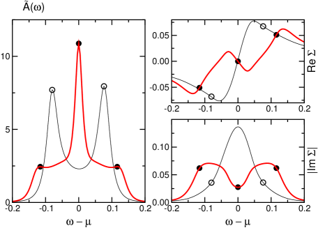
The appearance of the antiadiabatic central peak is first illustrated in the renormalized spectral density of Fig. 2 for a particularly simple parametrization. We put and , so that the unperturbed system has a square nested Fermi surface touching the vH singularity. The product is taken as constant, independent of the position on the Fermi surface. The band-edge eV eV eV is set to the low-temperature regime, as in the rest of the article, while the remaining parameters are irrelevant for the discussion. The thin line in the left panel gives the spectral strength at , simply split into two peaks. They have quasiparticle signatures, as shown in the right two panels: has a negative slope at the peak positions, and is small.
The thick lines show the situation at , the vH point, for the same parametrization. The maxima in the side wings, also denoted by full circles, are evidently incoherent: the corresponding has a positive slope, and is large. Clearly a central peak has survived at the vH point, protected by the antiadiabatic mechanism. To see this, note that when the boson response is peaked around in Eq. (5), the main contribution to at , the vH point, comes from electrons at , the other vH point, where they are slow.
Thus the central peak consists of vH electrons which do not scatter because they barely move, so for them even the slowest available paramagnons are averaged out; this is the antiadiabatic regime. It is clear that it violates the Fermi liquid paradigm, since at the Fermi level despite . This is because electrons interact with dissipative bosons. When the boson damping is zero, for at the vH point itself; this was checked analytically Sunko and Barišić (1993). It is further important to note that the antiadiabatic peak does not necessarily appear at the Fermi level, since it has its own -dispersion. In the zone, and for the antiadiabatic peak behave similarly as for a quasiparticle, including the reduced but finite quasiparticle weight. We shall see that the peak can reveal its antiadiabatic origin nevertheless, by disappearing with changing when the electrons involved acquire a significant velocity.
Our calculation can support various physically motivated notions of a pseudogap simply by performing it in different regions of parameter space. Because of this, the actual pseudogap obtained in a particular calculation with realistic parameters usually behaves as a transitional form between intuitive limiting cases. For example, one might say that a pseudogap exists only if the central peak does not cross the Fermi energy. However, that behavior continuously transforms into the usual quasiparticle one simply by increasing the energy of the paramagnon band-edge, and in fact the central peak can easily cross before the side wings have disappeared. Similarly, the notion that has to have a positive slope for a side wing to be called incoherent is less restrictive than requiring to be maximal at the peak position. Thus the latter notion of incoherence is found as a limiting case, while the former appears across a wide range of parametrizations. Finally, one could define the pseudogap by the spectral weight having a minimum at the Fermi energy, and a maximum in at the same position. The split quasiparticle (thin line) in the left panel of Fig. 2 is a limiting case for such a definition, where all the peaks appearing are coherent. However, these peaks do not cross the Fermi energy. This corresponds to the most common understanding of a pseudogap, where a coherent quasiparticle splits in two because of strong scattering at , which is the precursor to the new zone boundary when at fixed temperature.
Let us narrow the usage of the term ‘pseudogap’ now, to the one found relevant for the present work. We do not call the thin line in the left panel of Fig. 2 a pseudogap, in spite of the valley between the two peaks, corresponding to a large . However, the peaks themselves are ‘coherent,’ as discussed above. Here we reserve the term ‘pseudogap’ for manifestly incoherent side wings, like the side wings of the thick line, irrespective of the nature or presence of a central peak in the middle. Notably, other parametrizations can give three coherent peaks at the vH point, the two side ones like at the nodal point, and an antiadiabatic one in the middle; in that case there is no pseudogap at all, in the language of this article.
III Model regimes
At fixed low temperature, the ratio of the paramagnon ‘band-edge’ to the damping becomes the principal physical parameter of the self-energy (5). We shall show below that this number is relevant to account for the principal features of the ARPES measurements in BSCCO and YBCO Lu et al. (2001) along the – line, which we shall call X–M, in accord with the crystallographic notation for YBCO. We take to be 40 meV, in accord with experiment, which puts our calculation in the low-temperature limit, . This means that the electrons are only perturbed by paramagnon zero-point motion. We argue below it is this ‘quantum’ pseudogap which is actually observed in optimally doped BSCCO. The use of the term pseudogap to refer to the destruction of the Fermi liquid behavior by magnetic quantum fluctuations is already well established in studies of the antiferromagnetic quantum critical point Coleman (1999).
The parameters in expression (5) are treated semiphenomenologically, i.e. we shall use them primarily to adjust the experimentally observed outcomes, but with regard to physically reasonable values. Let us give a standard parametrization now, used throughout the article. The renormalized parameters of the Emery model in the hole picture are: copper-oxygen hopping eV, oxygen-oxygen hopping eV, and effective copper-oxygen energy splitting eV. The Fermi energy is in the electron antibonding band (1) of the three-band model Mrkonjić and Barišić (2003a). The temperature is eV, as already mentioned.
The paramagnon parameters are the band-edge eV, damping eV, cutoff eV, and correlation length 3 lattice spacings. The coupling constant is eV. Its wave-vector dependence is neglected, because we concentrate on and . To get a feeling for it, we note that the total range of around the Fermi surface is 0.1 eV for this parametrization, which is roughly an order below the width of the non-interacting antibonding band (1). Hence eV may conveniently be imagined as ‘percent’ of the non-interacting electronic scale. The chemical potential is eV from the vH point. (Larger means less holes.) Individual parameter values are quoted elsewhere in the paper only to denote deviations from the set given here.
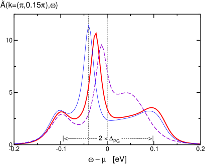
The generic form of the pseudogapped spectral function with a central peak is shown in Fig. 3. As long as we are in the vicinity of the vH point, some of the spectral strength of the slow electrons survives in the middle of the pseudogap, itself of width , near the Fermi energy. The persistence of a central peak in the single-loop approximation was noted earlier Bjeliš and S. Barišić (1975); Sunko and Barišić (1993). There appears an intrinsic ‘leading edge’ scale, the small distance from the central peak to the Fermi energy. When the chemical potential is shifted toward underdoping, this distance increases. The high background observed in ARPES does not appear here. It was obtained in both ARPES de Melo and Doniach (1990) and Raman Nikšić et al. (1995) contexts by taking into account the high-frequency slave-boson fluctuations in the charge channel, which we do not consider here. (In the latter case Nikšić et al. (1995) this was done in the so-called non-crossing approximation, a somewhat different starting point from the mean-field slave-boson one, on which this article is based.) The upper and lower wings at may be understood in the semiclassical language as a consequence of the electronic scattering on the nearly static, but still not completely ordered AF-like potential induced by the paramagnons. This interpretation implies essentially incoherent side wings, with a large and with a positive slope. (In fact a different structure can also appear, with coherent side peaks, as mentioned in the discussion of Fig. 2.) In the parametrizations used here to compare with experiment, the side wings are in fact incoherent, while the physical regime is at low temperature.
The pseudogap in the high-temperature limit looks quite similar, as shown by the broken line in Fig. 3. In particular the energy scale of the side wings is easily adjusted to be the same. The qualitative behavior is however different, and since the distinction is important for the phenomenology, we discuss it now.

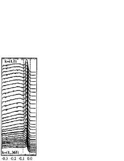
In Fig. 4, we show the calculated low-temperature (left panel) and high-temperature (middle and right panels) peaks dispersing along the X–M line. We first take the band-edge rather high, eV, to emphasize the antiadiabatic peak, which picks up most of the spectral strength. Then the only difference between the left and middle panels is the temperature, and we note that the antiadiabatic peak is much less dispersive in the low-temperature case, and loses strength before crossing the Fermi level. The low-temperature regime is influenced by both terms in Eq. (5) equally, with a competition between the Bose and Fermi contributions. In the high-temperature limit the second (boson response) term takes over, with a different dynamics, due to the fact that when , in Eq. (5) becomes , introducing an additional dispersive factor in the denominator. Note, however, that the intensities are given without the Fermi occupation factor — we show the renormalized spectral density , not . This means in particular that the loss of intensity in the left panel is not due to the Fermi surface crossing, in fact we shall see (Fig. 8 in the experimental section) that it occurs just as well when the antiadiabatic peak stays away from the Fermi surface.
It is possible to keep the antiadiabatic peak below the Fermi energy in the high-temperature regime as well, by lowering the band-edge . This is shown in the right panel. Notice that lowering the band-edge in the high temperature regime goes toward the opening of a true gap, so the antiadiabatic signal is much smaller, relative to the side wings. Otherwise, the dispersion is qualitatively similar to the left panel, especially so when we realize that lowering the band-edge flattens the dispersion in the low-temperature case as well (as visible in Fig. 8), similarly pushing the signal away from the Fermi energy. The important qualitative difference in the behavior of spectral strengths is however the following: in the left panel of Fig. 4, we notice that the side signal disappears before the antiadiabatic one; in the right panel, they disappear together. In fact, the generic behavior in the high-temperature limit is rather that the antiadiabatic peak disappears sooner. We shall see in the next section that experimental evidence in the superconducting state exhibits the low-temperature behavior, providing one piece of evidence that the measured response is in the low-temperature quantum regime.
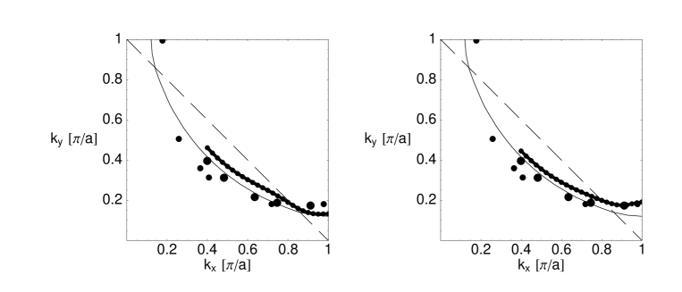
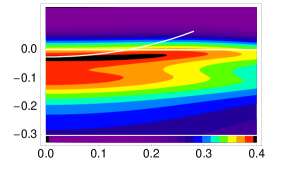
The second piece of evidence is the effect of the magnon perturbation on the Fermi surface. In the absence of a quasiparticle crossing, the experimental community has developed various alternative criteria to define the Fermi surface, one of which is the position of the maximum in the momentum-distribution curve at fixed Kaminski et al. (2001). We adopt that criterion in Fig. 5, which shows that the effect of magnon perturbation on the zeroth-order Fermi surface is qualitatively different for the high- and low-temperature pseudogaps. In the high-temperature (semiclassical) regime (left panel), the tendency is to change the shape of the Fermi surface so as to follow the zone diagonal in the vicinity of the ‘hot spots’ Coleman (1999), i.e. the points of intersection of the Fermi surface with the diagonal. Geometrically, this means that the angle of the Fermi surface with the zone diagonal decreases. In the low-temperature (quantum) regime , shown in the right panel, the result is precisely the opposite, the intersection angle increases, and there is even a tendency to turn the effective Fermi surface upwards, resulting in a ‘flared’ shape. While our parametrization was chosen for a best fit to energy distribution curves (see below), and we do not expect detailed agreement with the Fermi surface shape, this qualitative difference is of foremost physical importance. It shows, in effect, that ‘hot spot’ scenarios, for example Ref. Yanase and Yamada (1999), correspond to the high-temperature regime of Eq. (5). They depend on the similarity between ‘strong’ and ‘singular’ scattering at the nesting wave vector, but this similarity is qualitatively correct only when , which is not the observed case. The tendency of the Fermi surface to follow the zone diagonal for is of course a precursor to the diagonal becoming the new zone boundary, when the paramagnons condense. As already stressed above, this can only happen in the present model when . While the upturn of the Fermi surface has never been clearly observed — there is only one experiment Norman et al. (1995), the small points Fig. 5, which seems to show such a tendency — the bending to follow the zone diagonal can be excluded with certainty. The Fermi surface of optimally doped BSCCO in the vicinity of the vH points is at least a straight line parallel to the –X line. The marked difference between the two final shapes (thick lines) in Fig. 5 means that in the present model one must choose the right-hand panel to reproduce the experimentally observed shape. Thus, both the evolution of ARPES spectra in the Brillouin zone and correction to the zeroth order shape of the Fermi surface in BSCCO seem to point in the same direction, that the observed pseudogap is due to zero-point motion of the magnons.
This discussion can be followed in the form of Eq. 5. In the semiclassical regime , the first term is negligible with respect to the divergence of the boson occupation number in the second term, which is a precursor to the true gap. In the low-temperature regime, the two terms are of the same order. They contribute even at zero temperature, because the paramagnon zero-point motion can excite electrons within meV of the Fermi energy, and since the vH singularity is roughly within this range, that means a lot of them. Thus we can violate the conventional Fermi liquid picture simply by putting in dissipative paramagnons and letting , keeping at its observed value, as discussed on the simple example of Fig. 2. It would of course be interesting to understand why the paramagnon resonance should appear when the system goes superconducting. We hope to shed more light on this question when we consider the on-site repulsion explicitly, as mentioned in Sect. II.
IV Comparison with experimental spectra
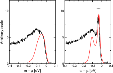
In Fig. 6, we show the comparison with experiment, used to establish the parametrization. The jagged lines are measured ARPES intensities Fedorov et al. (1999) of optimally doped BSCCO, integrated along the – line, in the normal (T=103 K, left) and superconducting state (T=46 K, right). The smooth lines are both calculated at the point with the parameters in the text, the only difference being the paramagnon damping: left, overdamped ( eV), right, underdamped ( eV). The difference, marked by crosses, in the positions of the leading peaks in the right panel is 100 K, the superconducting scale. The vertical scales of the two experimental and the two theoretical curves are the same, while the relative scale of theory vs. experiment is arbitrary. The single (overdamped) peak in the left panel and the side peak in the right panel correspond to a positive slope of and large , i.e. are both incoherent. Only the narrow (leading-edge) peak in the right panel is coherent, with negative slope of and small .
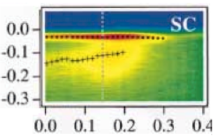
Having fixed all parameters at the point in Fig. 6, we now compare model predictions of evolution in the BZ with a different set of experimental data Kaminski et al. (2001), first in Fig. 7. The strong non-dispersive structure observed at the Fermi level corresponds to the antiadiabatic peak in the calculation. The lower wing of the pseudogap is shifted away from the position of the original three-band dispersion, reproducing the experimental high-energy ‘hump’ scale of 100 meV. The ridge at 100 meV binding roughly follows the original dispersion, broken and shifted by the paramagnon interaction. The antiadiabatic peak is interpolated between it and the upper wing (not visible because of the Fermi factor). Notably, the same behavior has been reported along the X–M line in YBCO Lu et al. (2001).
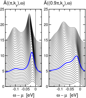
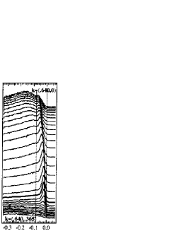
In Fig. 8, we show the detailed energy distribution curves (EDC‘s) corresponding to Fig. 7. All the qualitative experimental features are correctly reproduced: both the major and minor energy scales, and the downturn (in energy) of the antiadiabatic peak as one moves further away from the Fermi crossing. Such an approaching-then-receding of the narrow peak with respect to the Fermi level has been noticed in experiment Kaminski et al. (2001), and becomes more pronounced with underdoping.
The reference position of the central peak at is at the Fermi energy, as observed in our simple example in Fig. 2. As soon as the chemical potential is shifted, or one looks at other points in the BZ, the peak moves away from the Fermi energy, producing a ‘leading-edge’ energy scale of the order of the chemical potential, affected of course by its own dispersion. It is unrelated either to the primary AF scale, which determines the width of the pseudogap by the ‘high-energy’ side lobes, or the superconducting scale, which does not appear in the calculation at all. Of course, as the coupling constant decreases, or band-edge increases, the peak begins to turn back into an ordinary (weak-coupling) quasiparticle.
In the right two panels of Fig. 8, we show what happens as one moves towards the point in cuts parallel to the X–M line. We note a significant redistribution of spectral strength, such that the side peak is much stronger at , the –X line itself, but quickly loses strength as one moves perpendicularly away from it in the direction, parallel to the X–M line. Finally at , only the antiadiabatic peak survives. Experimentally, much the same behavior has been observed, with the proviso that it seems to evolve more slowly in the direction, so the qualitative features we calculate around here are observed around in experiment Kaminski et al. (2001). Again, the wide peak has its own approaching-then-receding sequence, similar to the one observed both in optimally doped Kaminski et al. (2001) and underdoped samples Campuzano et al. (1999). The fact that the calculated qualitative features continue to match closely the experimental situation as one moves away from the X–M line into the zone interior, while the quantitative evolution proceeds at a different pace, is possibly due to neglecting the -dependence of the product in the calculation.
The principal outcome of the comparison with experiment is that the experimental situation Kaminski et al. (2001) in the superconducting state corresponds to the model regime of low temperature and low damping . This allows us to claim that the pseudogapped regime in fact extends to optimal doping. Furthermore, the fact that our underdamped curves are calculated in the normal state means that the main qualitative effect of superconductivity on the ARPES signal is due to the reduction of magnon damping in the superconducting state.
V Summary
The present work associates the observed spectra around the vH point with the concept of an antiadiabatic central peak. It appears in the middle of a pseudogap, representing that part of the spectral strength which is not suppressed by the usual adiabatic mechanism of the opening of a pseudogap. The underlying main AF scale is allways that of the side wings in Fig. 3, which is observed in ARPES as a ‘high-energy’ feature, or ‘hump.’ In this way we are able to claim that the leading-edge scale, connected with the narrow peak, is not due to any independent physical phenomenon. The position of the antiadiabatic peak is sensitive to the chemical potential, which naturally accounts in our scheme for the increase of the ‘leading edge’ pseudogap with underdoping. We can easily recover the conventional Fermi liquid by raising the paramagnon band-edge or lowering the coupling constant. At some point the ‘hump’ scale goes to zero, and one recovers the usual weakly perturbed quasiparticle. This is consistent with the observation that the T* scale disappears at overdoping, rather than merging with the superconducting scale Loram et al. (2000); Ozyuzer et al. (2003).
The pseudogap with an antiadiabatic peak was found in this work to have two physical regimes, low- and high-temperature, relative to the paramagnon band-edge. The regime of low temperature corresponds to experiment in optimally doped BSCCO. In the model, it gives rise to a dispersion for the antiadiabatic peak which is qualitatively different from the bare one, amounting to a non-dispersive ‘feature’ at a few tens of meV binding energy. Thus the observed leading-edge scale need not be entirely due to the superconducting gap. The low-temperature regime is pseudogapped, because a true gap appears when before , i.e. it is always in the high-temperature regime. As long as is held fixed, a pseudogap-like situation will occur for , without developing into a true gap even for the lowest temperatures. However, it may be a true pseudogap, in the sense that the side wings are incoherent, and this is the case in the parametrization used here to compare with experiment. Lowering the band-edge in the low-temperature regime makes the central peak disappear just like in the high-temperature case, thus naturally accounting for the underdoped situation.
We took much trouble with Figs. 4 and 5 to choose the low-temperature regime, although the magnon mode at 41 meV is obviously much higher than the temperature. The reason is that our calculation is so simple and generic that it fairly represents the perturbation by any bosonic mode which does not have a slow component. There are a number of observed low-energy fluctuations, such as stripes, which we do not take into account here. At present, we cannot completely exclude a possible role of slow (spin) fluctuations in the electron response measured by ARPES. These can be modelled to some extent by a ‘central peak’ in the boson response, distinct from the dispersive branches studied here, and easily introduced in our calculation by a slightly more general parametrization Bjeliš and S. Barišić (1975) of . However, since the observed spectral strength redistribution and Fermi surface shape both correspond to our low-temperature regime, we can ascribe the main features of the ARPES response to the dispersive paramagnons. In this way the other low-energy phenomena are relegated to a secodary role, possibly having to do with the shape and spectral composition of the side wings. Even if the pseudogap were not due to paramagnons, still the conclusion would remain that the characteristic energy scale of the relevant boson is higher than the temperature, hence the pseudogap need not of itself imply any additional ground-state phenomena. As things stand, we see no reason to depart essentially from the natural interpretation in terms of AF paramagnons.
The neglected quantum fluctuations in the charge channel are also expected to affect the width and shape of the high-energy hump observed in ARPES, which appears sharper and narrower in our calculation than in experiment. Apart from that, the EDC‘s obtained along the X–M line have a striking resemblance to experiment in their main features. Both the high-energy scale of 100 meV, and the leading-edge scale of 20–30 meV are correctly reproduced. The main intensity pattern, where the peak loses strength further away from the vH point, without ever crossing the Fermi energy, is reproduced as well. The intensity shifts between the central peak and side wings are also obtained. Finally, the observed slight variation in the narrow peak position, which approaches the Fermi energy and then recedes from it, is also found in the calculation. Thus we believe that we have understood the physical origin of the narrow lowest-energy signal along the X–M line to be quite general: the electrons giving rise to this signal are slower than the perturbing paramagnons, and so escape the adiabatic suppression which opens the pseudogap. We can easily recover the actual experimental situation for , simply by overdamping the paramagnons, which washes out the antiadiabatic peak. This scenario is naturally consistent with the fact that a precursor of the narrow peak is sometimes observed above Tc. Based on the above discussion, we claim that the pseudogap in optimally doped BSCCO is in fact fully developed, of the order of 1000 K, and is only masked by the antiadiabatic peak. In this way we can view the superconducting correlations as a third scale, an order of magnitude lower than the pseudogap ‘hump’ scale, and two orders of magnitude below the on-site repulsion, here taken into account through the overall band renormalization. Their interplay with the antiadiabatic leading-edge scale found here, which is of the same order of 10 meV, should be of interest. It remains to be seen whether the physical regime found here to be relevant for the low-energy cuprate phenomenology can be consistently obtained from a microscopic strong-coupling approach in the presence of an oxygen-oxygen overlap, as outlined in Section II.
To conclude, we described the main low-energy signal along the X–M line in optimally doped BSCCO to be due to an antiadiabatic central peak. The pseudogap in the same material is an order of magnitude above the superconducting scale, and persists below Tc. The small separation between the antiadiabatic peak and the Fermi level appears naturally in the calculation, even in the absence of explicit superconductivity. It is primarily determined by the value of the chemical potential, in a way consistent with its observed variation with doping.
Acknowledgements.
Conversations with J. Friedel and E. Tutiš are gratefully acknowledged. This work was supported by the Croatian Government under Project .References
- Fretwell et al. (2000) H. M. Fretwell, A. Kaminski, J. Mesot, J. C. Campuzano, M. R. Norman, M. Randeria, T. S. R. Gatt, T. Takahashi, and K. Kadowaki, Phys. Rev. Lett. 84, 4449 (2000).
- Valla et al. (1999) T. Valla, A. V. Fedorov, P. D. Johnson, B. O. Wells, S. L. Hulbert, Q. Li, G. D. Gu, and N. Koshizuka, Science 285, 2110 (1999).
- Kivelson et al. (2003) S. A. Kivelson, I. P. Bindloss, E. Fradkin, V. Oganesyan, J. M. Tranquada, A. Kapitulnik, and C. Howald, Rev. Mod. Phys. 75, 1201 (2003).
- Sadovskii (2001) M. V. Sadovskii, Uspekhi fizicheskih nauk 171, 539 (2001).
- Lanzara et al. (2001) A. Lanzara, P. V. Bogdanov, X. J. Zhou, S. A. Kellar, D. L. Feng, E. D. Lu, T. Yoshida, H. Eisaki, A. Fujimori, K. Kishio, et al., Nature 412, 510 (2001).
- Ong et al. (2004) N. P. Ong, Y. Wang, S. Ono, Y. Ando, and S. Uchida, Ann. Phys.-Berlin 13, 9 (2004).
- Shen et al. (1995) Z. X. Shen, W. E. Spicer, D. M. King, D. S. Dessau, and B. O. Wells, Science 267, 343 (1995).
- Kim et al. (1998) C. Kim, P. J. White, Z. X. Shen, T. Tohyama, Y. Shibata, S. Maekawa, B. O. Wells, Y. J. Kim, R. J. Birgeneau, and M. A. Kastner, Phys. Rev. Lett. 80, 4245 (1998).
- Schabel et al. (1998) M. C. Schabel, C.-H. Park, A. Matsuura, Z. X. Shen, D. A. Bonn, R. Liang, and W. N. Hardy, Phys. Rev. B57, 6090 (1998).
- Fedorov et al. (1999) A. V. Fedorov, T. Valla, P. D. Johnson, Q. Li, G. D. Gu, and N. Koshizuka, Phys. Rev. Lett. 82, 2179 (1999).
- Feng et al. (2001) D. L. Feng, N. P. Armitage, D. H. Lu, A. Damascelli, J. P. Hu, P. Bogdanov, A. Lanzara, F. Ronning, K. M. Shen, H. Eisaki, et al., Phys. Rev. Lett. 86, 5550 (2001).
- Kaminski et al. (2001) A. Kaminski, M. Randeria, J. C. Campuzano, M. R. Norman, H. Fretwell, J. Mesot, T. Sato, T. Takahashi, and K. Kadowaki, Phys. Rev. Lett. 86, 1070 (2001).
- Mesot et al. (2001) J. Mesot, M. Randeria, M. R. Norman, A. Kaminski, H. M. Fretwell, J. C. Campuzano, H. Ding, T. Takeuchi, T. Sato, T. Yokoya, et al., Phys. Rev. B 63, 224516 (2001).
- Matsui et al. (2003) H. Matsui, T. Sato, T. Takahashi, S.-C. Wang, H.-B. Yang, H. Ding, T. Fujii, T. Watanabe, and A. Matsuda, Phys. Rev. Lett. 90, 217002 (2003).
- Campuzano et al. (2004, to appear) J. C. Campuzano, M. R. Norman, and M. Randeria, in The Physics of Superconductors Vol. II: Novel Superconductors: Cuprate, Heavy-Fermion, and Organic Superconductors, edited by K. H. Bennemann and J. B. Ketterson (Springer, 2004, to appear), cond-mat/0209476.
- Randeria (1998) M. Randeria, in Proceedings of the International School of Physics ’Enrico Fermi’ Course CXXXVI on High Temperature Superconductors, edited by G. Iadonisi, J. R. Schrieffer, and M. L. Chiafalo (IOS Press, 1998), pp. 53–75, cond-mat/9710223.
- Chuang et al. (2001) Y. D. Chuang, A. D. Gromko, A. Fedorov, Y. Aiura, K. Oka, Y. Ando, H. Eisaki, S. I. Uchida, and D. S. Dessau, Phys. Rev. Lett. 87, 117002 (2001).
- Kordyuk et al. (2002) A. A. Kordyuk, S. V. Borisenko, T. K. Kim, K. A. Nenkov, M. Knupfer, J. Fink, M. S. Golden, H. Berger, and R. Follath, Phys. Rev. Lett. 89, 077003 (2002).
- Vilk (1997) J. M. Vilk, Phys. Rev. B 55, 3870 (1997).
- Friedel and Kohmoto (2002) J. Friedel and M. Kohmoto, Eur. Phys. J. B 30, 427 (2002).
- Eschrig and Norman (2003) M. Eschrig and M. R. Norman, Phys. Rev. B 67, 144503/1 (2003).
- Emery (1987) V. J. Emery, Phys. Rev. Lett. 58, 2794 (1987).
- Mrkonjić and Barišić (2003a) I. Mrkonjić and S. Barišić, Eur. Phys. J. B 34, 69 (2003a).
- Falicov and Kimball (1969) L. M. Falicov and J. C. Kimball, Phys. Rev. Lett. 22, 997 (1969).
- Gor’kov and Sokol (1989) L. P. Gor’kov and A. V. Sokol, J. Physique 50, 2823 (1989).
- Sunko and Barišić (1996) D. K. Sunko and S. Barišić, Europhys. Lett. 36, 607 (1996), erratum: Europhys. Lett. 37, p. 313, 1997.
- Sunko (2000) D. K. Sunko, Fizika A (Zagreb) 8, 311 (2000), cond-mat/0005170.
- Freericks and Devereaux (2001) J. K. Freericks and T. P. Devereaux, Phys. Rev. B 64, 125110/1 (2001).
- Sunko (2005) D. K. Sunko, Eur. Phys. J. B 43, 319 (2005).
- Mrkonjić and Barišić (2003b) I. Mrkonjić and S. Barišić, Eur. Phys. J. B 34, 441 (2003b).
- Mrkonjić and Barišić (2004) I. Mrkonjić and S. Barišić, Phys. Rev. Lett. 92, 129701/1 (2004).
- Andersenn et al. (1995) O. K. Andersenn, A. I. Liechtenstein, O. Jepsen, and F. Paulsen, J. Phys. Chem. Solids 56, 1573 (1995).
- Tutiš (1994) E. Tutiš, Ph.D. thesis, University of Zagreb (1994), in Croatian.
- Dzyaloshinskii and Yakovenko (1988) I. E. Dzyaloshinskii and V. M. Yakovenko, Int. J. Mod. Phys. B 5, 667 (1988).
- Vilk and Tremblay (1997) J. M. Vilk and A. S. Tremblay, J. Phys. I France 7, 1309 (1997).
- Yanase (2004) Y. Yanase, J. Phys. Soc. Jpn. 73, 1000 (2004).
- Rossat-Mignod et al. (1991) J. Rossat-Mignod, L. P. Regnault, C. Vettier, P. Burlet, J. Y. Henry, and G. Lapertot, Physica B 169, 58 (1991).
- Ishida et al. (1996) K. Ishida, Y. Kitaoka, K. Asayama, K. Kadowaki, and T. Mochiku, Physica C 263, 371 (1996).
- Gor’kov and Teitel’baum (2004) L. P. Gor’kov and G. B. Teitel’baum, JETP Lett. 80, 195 (2004), cond-mat/0312379.
- Bjeliš and S. Barišić (1975) A. Bjeliš and S. Barišić, J. Physique Lett. 36, L169 (1975).
- Morr (2000) D. K. Morr, Physica B 280, 178 (2000).
- Abrikosov et al. (1975) A. A. Abrikosov, L. P. Gorkov, and I. E. Dzaloshinski, Methods of Quantum Field Theory in Statistical Physics (Dover, 1975).
- Sunko and Barišić (1993) D. K. Sunko and S. Barišić, Europhys. Lett. 22, 299 (1993).
- Brazovskii and Dzyaloshinskii (1976) S. A. Brazovskii and I. E. Dzyaloshinskii, ZhETF 71, 2338 (1976).
- Lu et al. (2001) D. H. Lu, D. L. Feng, N. P. Armitage, K. M. Shen, A. Damascelli, C. Kim, F. Ronning, and Z.-X. Shen, Phys. Rev. Lett. 86, 4370 (2001).
- Coleman (1999) P. Coleman, Physica B 259-261, 353 (1999).
- de Melo and Doniach (1990) C. A. R. S. de Melo and S. Doniach, Phys. Rev. B 41, 6633 (1990).
- Nikšić et al. (1995) H. Nikšić, E. Tutiš, and S. Barišić, Physica C 241, 247 (1995).
- Valla et al. (2000) T. Valla, A. V. Fedorov, P. D. Johnson, Q. Li, G. D. Gu, and N. Koshizuka, Phys. Rev. Lett. 85, 828 (2000).
- Norman et al. (1995) M. R. Norman, M. Randeria, H. Ding, and J. C. Campuzano, Phys. Rev. B 52, 615 (1995).
- Yanase and Yamada (1999) Y. Yanase and K. Yamada, J. Phys. Soc. Jpn. 68, 548 (1999).
- Campuzano et al. (1999) J. C. Campuzano, H. Ding, M. R. Norman, H. M. Fretwell, M. Randeria, A. Kaminski, J. Mesot, T. Takeuchi, T. Sato, T. Yokoya, et al., Phys. Rev. Lett. 83, 3709 (1999).
- Loram et al. (2000) J. W. Loram, J. L. Luo, J. R. Cooper, W. Y. Liang, and J. L. Tallon, Physica C 341-348, 831 (2000).
- Ozyuzer et al. (2003) L. Ozyuzer, J. E. Zasadzinski, K. E. Gray, D. G. Hinks, and N. Miyakawa, IEEE Transactions on Applied Superconductivity 13, 893 (2003), cond/mat-0301335.