Electron properties of carbon nanotubes in a periodic potential

Abstract

A periodic potential applied to a nanotube is shown to lock electrons into incompressible states that can form a devil’s staircase. Electron interactions result in spectral gaps when the electron density (relative to a half-filled Carbon $\pi-$band) is a rational number per potential period, in contrast to the single-particle case where only the integer-density gaps are allowed. When electrons are weakly bound to the potential, incompressible states arise due to Bragg diffraction in the Luttinger liquid. Charge gaps are enhanced due to quantum fluctuations, whereas neutral excitations are governed by an effective SU(4)$\simeq$O(6) Gross-Neveu Lagrangian. In the opposite limit of the tightly bound electrons, effects of exchange are unimportant, and the system behaves as a single fermion mode that represents a Wigner crystal pinned by the external potential, with the gaps dominated by the Coulomb repulsion. The phase diagram is drawn using the effective spinless Dirac Hamiltonian derived in this limit. Incompressible states can be detected in the adiabatic transport setup realized by a slowly moving potential wave, with electron interactions providing the possibility of pumping of a fraction of an electron per cycle (equivalently, in pumping at a fraction of the base frequency).

I Introduction

Since their discovery,Iijima carbon nanotubes (NTs) remain in focus of both basic and applied research. Dresselhaus ; AvourisDresselhaus Besides their important technological potential, McEuen'98 ; Dekker'99 nanotubes are a testing ground for novel physical phenomena involving strong electron interactions. In particular, they are believed to be perfect systems to study Tomonaga-Luttinger liquid effects. Krotov'97 ; Kane'97 ; Egger'97 ; Odintsov'99 ; Levitov'01 ; Stone Experimentally, effects of electron-electron interactions in nanotubes have been observed in the Coulomb blockade peaks in transport, Bockrath'97 ; Tans'98 in the power law temperature and bias dependence of the tunneling conductance,Bockrath'99 ; Yao'99 ; Nygard and in the power law dependence of the angle-integrated photoemission spectra.PE

Nanotubes are rich systems to study electron correlations for a number of reasons. Indeed, their one-dimensional (1d) character increases effects of interactions; spin and Brillouin zone degeneracyDresselhaus result in the presence of the four polarizations of Dirac fermions which can allow one to probe SU(4) spin excitations; Levitov'01 ; SU4Kondo-exp ; SU4Kondo-th exceptional chemical and mechanical NT properties result in very low disorder; finally, diverse methods of nanotube synthesis, a variety of available nanotube chiralities and of the ways of coupling to the nanotube electron system allow one to explore a wide region of parameter space.

In the present work we propose to employ the coupling of an external periodic potential to the nanotube electronic system as a probe of both Tomonaga-Luttinger correlations, and of the 1d Wigner crystallization, via commensurability effects. We focus on the electron properties of single-wall NTs in a periodic potential whose period $\lambda_{\rm ext}$ is much greater than the NT radius $a$, $\lambda_{\rm ext}\gg a$. Such a potential can be realized using optical methods, by gating, or by an acoustic field. In all of these cases, the realistic period $\lambda_{\rm ext}$ is of the order 0.1–1 $\mu$m. As shown below, effects of the Tomonaga-Luttinger correlations on the Bragg diffraction of electrons, realization of the SU(4) spin excitations, as well as pinning of the Wigner crystal can be demonstrated in such a setup depending on the applied potential and on the NT parameters.

In particular, below we will identify incompressible electron states, characterized by excitation gaps, that can arise when the average NT electron number density $\bar{\rho}$ (counted from half-filling) is commensurate with the period $\lambda_{\rm ext}$ of the external potential:

$$\bar{\rho}={m_{\rm tot}\over\lambda_{\rm ext}}\,,\quad m_{\rm tot}=4m\,.$$ (1)

In Eq. (1), $m$ is the number of fermions of each of the four polarizations (herein called “flavors”) per period.

At what density values $m$ can the spectral gaps open? The single-particle treatmentTalyanskii'01 maps the problem onto that of the Bloch electron, resulting in the spectrum of minibands separated by minigaps as a consequence of the Bragg diffraction on the external potential. Filling up an integer number $m$ of minibands corresponds to adding $m$ electrons of each flavor per “unit cell” (the period $\lambda_{\rm ext}$). Thus, minigaps open up when the density (1) is integer: $m=0,\,\pm 1,\,\pm 2,\,...$ .Talyanskii'01 In other words, the wave nature of the Bloch electron leads to commensurate states with integer density.

Our main result here is that electron interactions dramatically change the spectrum, adding incompressible states at rational densities $m=p/q$, in which commensurability is induced by interactions. NT-devil In a fractional$-m$ state, the NT electron system is locked by the external potential into a $q\lambda_{\rm ext}-$periodic commensurate configuration (such as the ones schematically represented in Fig. 1). Naturally, the states with the lower denominator $q$ are more pronounced. Realistically, due to finite NT length and temperature, only a few states with small enough $q$ can be detected. However, these fractional-$m$ states are important as the corresponding minigaps are interaction-induced (and vanish in the noninteracting limit). Measurement of such minigaps can provide a direct probe of interactions between electrons.

(a)                                                                    
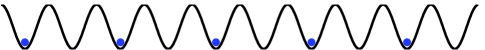
(b)                                                                    
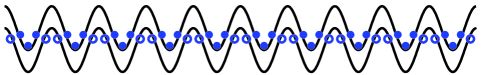
(c)                                                                    
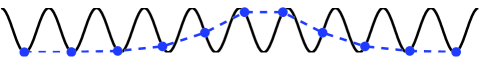
(d)                                                                    
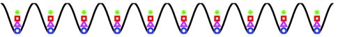
(e)                                                                    

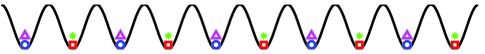
Figure 1: (Color online) Incompressible electron states (schematic). (a) The $(1/2,0)$ state with $m_{\rm tot}=1/2$. (b) The $(3,2)$ state with $m_{\rm tot}=1$. Large potential amplitude breaks the “Dirac vacuum” placing holes (open circles) into the potential maxima. (c) An example of the phase soliton excitation over the $(1,0)$ state. The excitation gap is given by the phase soliton energy. (d) The $m=1$ incompressible state allowed by the Bloch theory of noninteracting nanotube electrons. Four kinds of labels mark the NT fermions of the four flavors. (e) Semiclassical picture of the simplest interaction-induced $m=1/2$ state. Fermions of the same flavor avoid each other due to the Pauli principle.

From a practical standpoint, measurement of the gaps can identify the incompressible states characterized by quantum coherence on a macroscopic scale. A challenging experimental proposalTalyanskii'01 is to realize the Thouless pumpThouless by taking advantage of the semi-metallic NT dispersion. In such a setup, a quantized current is predicted to arise whenever the chemical potential is inside the minigap created by the adiabatically slowly moving potential wave. As our approach suggests, due to electron interactions, commensurability (1) will result in additional current plateausNT-devil corresponding to pumping on average of a fraction of unit charge per cycle. Equivalently, electron interactions could allow one to realize a novel effect of adiabatic pumping of charge at the fraction of the base frequency of the potential modulation.

In connection with the adiabatic current quantization, we note a parallel between our system and the quantum Hall effect. In both cases, commensurability with external electromagnetic field yields incompressible states, spectral gaps, and quantization in transport. Moreover, it is the electron interactions that result in the incompressible states at fractional filling factors (commensuration due to interactions) in addition to the integer plateaus (commensuration due to wave nature of electrons), both causing non-dissipative transport.Kane-Lubensky This similarity extends onto the disorder stabilizing plateaus at lower denominators.

From a theoretical viewpoint, the excitation spectrum is linked to the general theory of commensurate-incommensurate transitions. Frenkel ; FvdM ; Dzyal ; Pokrovsky ; Bak In this approach, an excitation over the commensurate state (an incommensuration) is represented by a phase soliton [illustrated in Fig. 1(c)], whose energy gives the corresponding spectral gap. In the present work the phase soliton method is generalized onto the case of strongly interacting massive Dirac fermions of multiple polarizations.

Technically, the problem at hand requires non-perturbative treatment of electron interactions at low density ($\bar{\rho}\lambda_{\rm ext}=m_{\rm tot}\sim 1$), i.e. at the bottom of the band, taking into account the effects of the curvature of the electronic dispersion. This is hard to achieve in the conventional bosonization scheme which rests on the linearized dispersion and describes hydrodynamic density modes extended over the whole system. Indeed, the curvature of the dispersion is a “dangerously irrelevant perturbation” that causes ultraviolet divergencies. However, it is the curvature of the dispersion that can provide a length scale to an otherwise scale-invariant Gaussian bosonic action. Not surprisingly, phenomena in which the physics on the scale of Fermi wavelength is important, such as the Coulomb drag between quantum wires,Drag often rely on the curvature and, hence, are difficult to treat.

Nanotubes provide a crucial theoretical advantage: Even massive interacting Dirac fermions can be bosonized, by virtue of the massive Thirring — sine-Gordon duality,Coleman ; Haldane with the curvature of the dispersion controlled by the Dirac mass (NT gap $\Delta_{0}$ at half-filling). In the bosonic language, the gap controls the strength of the nonlinear term in the bosonic action. Moreover, the NT Hamiltonian is SU(4) symmetric in the forward scattering approximation. This symmetry simplifies the treatment since in the problem of the four coupled modes, only two different length scales appear: The charge scale, ${l_{\rm ch}}$ (screening length for the Coulomb interaction), and the flavor scale, ${l_{\rm fl}}\ll{l_{\rm ch}}$, with a meaning of a size of the electronic wave function represented by a composite sine-Gordon soliton of the charge and flavor modes. Levitov'01

External periodic potential locks electrons into incompressible states at commensurate densities. As a semiclassical illustration of this phenomenon, in Fig. 1(d,e) the centers of solitons that represent electrons of the different flavors are marked by the four different symbols. In accord with the above, such a locking is only possible when the NT gap $\Delta_{0}\neq 0$, since the dispersion curvature gives rise to the finite soliton sizes ${l_{\rm ch}},{l_{\rm fl}}\propto\Delta_{0}^{-\gamma/2}$ with $\gamma>0$. For strictly linear dispersion (as in the armchair tube), both of these scales are infinite, and the minigaps do not open, as it is impossible to pin a system that has an infinite length scale.FSA

In general, both Bragg diffraction and the Coulomb interaction contribute to the excitation gaps. While the diffraction is a dominant factor for the incompressible states when the system is controlled by the Luttinger-liquid fixed point, the Coulomb interaction plays a major role when the electron system is in the Wigner-crystal regime. The external potential, by bringing the additional length scale $\lambda_{\rm ext}$ to the problem, naturally distinguishes between the two sides of the Luttinger-liquid – Wigner-crystal crossover. Technically, this distinction occurs on the level of a saddle point of the nonlinear bosonic action.

In a recent Letter, NT-devil we showed that, in the semiclassical (strong coupling) limit, when electrons are nearly pointlike (${l_{\rm fl}}\ll\lambda_{\rm ext}$), the long range Coulomb interaction leads to the devil’s staircase of commensurate states representing the pinned Wigner crystal. Gaps open at rational densities $m_{\rm tot}$, and Coulomb interaction sets the gap energy scale. An example of such a state with $m_{\rm tot}=1/2$ is shown schematically in Fig. 1(a). In this work we will study the phase diagram in this limit in detail. Remarkably, the Dirac character of nanotube electrons brings about a set of incompressible states in which the “Dirac vacuum” is broken when the potential amplitude exceeds the gap at half-filling. In this case, physically different incompressible states can correspond to the same total density (1) with

$$4m=m_{\rm tot}=n_{e}-n_{h}\,.$$ (2)

To further characterize these states we specify the pair of numbers $(n_{e},n_{h})$ of electrons and holes in the potential minima and maxima correspondingly. An example of the $(3,2)$ state with $m_{\rm tot}=1$ is schematically shown in Fig. 1(b).

The opposite limit of the weakly coupled electrons (${l_{\rm fl}}\gg\lambda_{\rm ext}$) is connected to the gaps opening due to the Bragg diffraction. In this case electrons are delocalized over many periods, and gaps occupy a small part of the spectrum. Exchange is important, and adds to the cost of an excitation in which an extra electron of a particular flavor is added to the commensurate configuration. Below we will specifically focus on the lowest-denominator fractional state $m=1/2$, for which we find the effective action that describes excitations over the commensurate state, and obtain the charge and the SU(4)–flavor excitation gaps.

This paper is organized as follows. In Section II we introduce the model Hamiltonian. In Section III, as a warm-up, we consider the noninteracting problem. In Section IV the many-body Hamiltonian is bosonized.

Section V is central, as we introduce the phase soliton method for the bosonized NT electrons. In Section VI we consider the Bragg diffraction limit, whereas in Section VII we focus on the pinned Wigner crystal. In Section VIII we outline the phase diagram in the semiclassical (Wigner crystal) limit. In Section IX we discuss experimental ways to detect incompressible states.

II The Model

Near half-filling, the nanotube electron system in the forward scattering approximationEgger'97 ; Kane'97 is described in terms of the four ($2_{\rm spin}\times 2_{\rm valley}$) Dirac fermion flavors, with the following second-quantized Hamiltonian,

$${\cal H}={\cal H}_{0}+{\cal H}_{\rm bs}+{\cal H}_{\rm ext}\,.$$ (3)

The first term ${\cal H}_{0}$ is the massless Dirac Hamiltonian that includes Coulomb repulsion:

$${\cal H}_{0}=-i\hbar v\int\sum_{\alpha=1}^{4}\psi^{+}_{\alpha}\sigma_{3}\partial_{x}\psi_{\alpha}dx+\frac{1}{2}\sum_{k}\rho_{k}V(k)\rho_{-k}\,.$$ (4)

Here

$$\psi_{\alpha}=\left(\matrix{\psi^{R}_{\alpha}\cr\psi^{L}_{\alpha}}\right)\,,\quad 1\leq\alpha\leq 4$$ (5)

is a two component Weyl spinor of the flavor $\alpha$, $x$ is the coordinate along the tube, $\sigma_{1,3}$ are the Pauli matrices, and $v\approx 8\cdot 10^{7}$ cm/s is the NT Fermi velocity. In the total number density $\rho_{k}=\int\!dx\,e^{-ikx}\rho(x)$, with

$$\rho(x)\simeq\sum_{\alpha=1}^{4}\psi^{+}_{\alpha}(x)\psi_{\alpha}(x)\,,$$ (6)

we neglected the strongly oscillating components $\sim e^{\pm 2iK_{\rm BZ}x}$, with $K_{\rm BZ}\sim 1/a_{\rm cc}$ defining the position of the Dirac points in the Brillouin zone of graphene [$a_{cc}=0.143$ nm being the length of the Carbon bond]. For a nanotube of radius $a$ placed on a substrate with the dielectric constant $\varepsilon$, the 1d Coulomb interaction

$$V(k)=\textstyle{\frac{2}{\varepsilon+1}V_{0}(k)}\,,$$ (7)

where

$$V_{0}(k)\simeq e^{2}\ln\left[1+(ka)^{-2}\right]\,.$$ (8)

The essence of the forward scattering approximation employed above is that even in the presence of electron interactions, the two Dirac points at the corners of the Brillouin zone remain decoupled. Since the long range potential (7) does not discriminate between the Carbon sublattices, scattering amplitudes for the fermions of same and opposite chiralities at each Dirac point are equal. Egger'97 ; Kane'97 Hence in the Hamiltonian (4) we include only the part of electron interaction that involves the smooth part (6) of the electron density. Furthermore, in the Hamiltonian (4) the backscattering and Umklapp processes between the Dirac points are discarded. These processes are parametrically reduced by $a_{cc}/a\lesssim 0.1$, while the Umklapp amplitude is also numerically small.Odintsov'99

The second term in the Hamiltonian (3) describes the backscattering between the left and right moving fermions within each Dirac point:

$${\cal H}_{\rm bs}=\Delta_{0}\int{\textstyle\sum_{\alpha=1}^{4}}\psi^{+}_{\alpha}\sigma_{1}\psi_{\alpha}dx\,.$$ (9)

This backscattering is different from the usual “$V(2k_{F})$” term in quantum wires, as the interaction-induced gaps are undetectably small in metallic NTs. Instead, we rely on the curvature of the dispersion arising from the bare gap $\Delta_{0}$ at half-filling. Remarkably, this gap can greatly vary depending on NT chirality or external fields.Dresselhaus In particular, semiconducting nanotubes have a large gap

$$\Delta_{0}^{\rm(semicond)}={\hbar v\over 3a}\simeq 0.18~{}{\rm eV}/a_{\rm[nm]}$$ (10)

that scales inversely with the radius $a$. Metallic NTs can be of the two kinds. There are truly metallic, or the so-called “armchair” NTs which have a zero gap at half-filling, $\Delta_{0}=0$. However, a gap $\Delta_{0}\ll D$ that is small compared to the 1d bandwidth

$$D={\hbar v\over a}=0.53~{}{\rm eV}/a_{\rm[nm]}$$ (11)

can appear due to the curvature of the 2d graphene sheet in the nominally metallic tube. This gap is inversely proportional to the square of the NT radius, and is numerically given by

$$\Delta_{0}^{\rm(semimet)}\approx 10~{}{\rm meV}\cdot|\cos 3\Theta_{\rm ch}|/a_{\rm[nm]}^{2}$$ (12)

as a function of the NT chiral angle $\Theta_{\rm ch}$. zigzag ; exp-curvature Even smaller $\Delta_{0}$ can be induced in a strictly metallic “armchair” ($\Theta_{\rm ch}=\pi/6$) tube by applying magnetic field parallel to the NT axis. B-paral ; exp-B-parallel

Finally, interaction with the external periodic potential is represented by

$${\cal H}_{\rm ext}=\int\!dx\,\rho\,U(x)\,.$$ (13)

In the present work, for the purpose of simpler algebra, we consider the potential of the form

$$U(x)=A\cos k_{\rm ext}x\,,\quad k_{\rm ext}={2\pi/\lambda_{\rm ext}}\,.$$ (14)

Qualitatively, the results of this work will be valid for any periodic potential realized by the means described in the Introduction. As the values of the period $\lambda_{\rm ext}$ are in the $0.1-1\,\mu$m range, the separation of scales $k_{\rm ext}\ll 1/a\ll 1/a_{cc}$ rules out a possibility of coupling between the Dirac points via the potential (14), in full compatibility with the forward scattering approximation.

In general, our main conclusion about the interaction-induced incompressible states at fractional densities that open up in addition to the integer-density gaps is valid for any value of the NT gap $\Delta_{0}$. Quantitatively, our present analysis that will be based on the bosonization demands the separation of scales $\Delta_{0}\ll D$, practically requiring the semimetallic tubes.

The Hamiltonian (3) written in the forward scattering approximation is SU(4) invariant with respect to rotations in the space of the fermion flavors $\psi_{\alpha}$, with both the Coulomb interaction and the coupling to the smooth external potential (14) preserving this symmetry.

III Noninteracting Electrons

In the absence of interactions, the contributions of the four fermion flavors factorize. Here we consider the single electron spectrum [cf. Eqs. (4), (9), and (13)]

$$\left\{{\cal H}_{D}+U(x)\right\}\psi=\epsilon\psi\,,$$ (15)

where ${\cal H}_{D}$ for fermions of each flavor is given by

$${\cal H}_{D}=-i\hbar v\,\sigma_{3}\partial_{x}+\Delta_{0}\,\sigma_{1}\,.$$ (16)

This spectrum has been briefly analyzed in Ref. Talyanskii'01, . Below we will study it in detail emphasizing the distinction between the two opposite regimes of coupling, tight-binding vs. nearly-free electrons. It is convenient to perform a gauge transformation

$$\psi^{\prime}(x)=e^{-i\bar{A}\sigma_{3}\sin k_{\rm ext}x}\,\psi(x)\,,$$ (17)

where the dimensionless amplitude

$$\bar{A}={A/\epsilon_{0}}\,.$$ (18)

The kinetic energy scale

$$\epsilon_{0}\equiv\hbar k_{\rm ext}v=hv/\lambda_{\rm ext}=3.3~{}{\rm meV}/{\lambda_{\rm ext}}_{\rm\,[\mu m]}$$ (19)

is the Dirac level spacing in each potential minimum.

After the gauge transformation (17) the Hamiltonian ${\cal H}_{D}+U(x)$ becomes

$${\cal H}^{\prime}=-i\hbar v\,\partial_{x}\sigma_{3}+\Delta_{0}\sigma_{1}e^{-2i\bar{A}\sigma_{3}\sin k_{\rm ext}x}\,.$$ (20)

Remarkably, due to the Dirac character of the problem, in the Hamiltonian (20) the relative importance of the potential energy (the second term) is governed by the value of the Dirac gap $\Delta_{0}$, rather than the potential amplitude $A$, whereas the kinetic energy (the first term) is ${\cal O}(\epsilon_{0})$. [Note that in Eq. (20) we discarded the Schwinger anomaly term $\propto\int\!dx\,U^{2}(x)$ since its effectNT-anom of adding a constant energy shift is not important here.]

The coupling of the NT electron to the external potential can be either weak or strong, depending on the gap value $\Delta_{0}$. Consider the eigenvalue problem

$${\cal H}^{\prime}\psi^{\prime}=\epsilon\psi^{\prime}$$ (21)

that is periodic in $\lambda_{\rm ext}$. Its solutions are the spinor Bloch states $\psi^{\prime}_{p}(x)=u_{p}(x)e^{ipx}$ with a quasimomentum $\hbar p$ taking values in the effective Brillouin zone defined by the potential period, $-k_{\rm ext}/2<p<k_{\rm ext}/2$. Below we distinguish between the weak coupling limit (nearly free electrons), and the strong coupling (tight-binding) limit.

In the limit of nearly free electrons,

$$\psi^{\prime}_{p}(x)=u_{p}(x)e^{ipx}\,,\quad u_{p}(x)\simeq{\rm const},$$ (22)

and the electron wave functions are close to plane waves. Note that in the massless case of $\Delta_{0}=0$, $u_{p}\equiv{\rm const}$, and the external potential has no effect since it is gauged away. It is a manifestation of the fact that the scalar external potential does not mix massless Dirac branches whose wave functions have a spinor structure. This is also consistent with the above discussion that the potential energy scale is determined by the backscattering $\Delta_{0}$.

When the backscattering $\Delta_{0}\neq 0$, Bragg diffraction on the potential results in mixing between the left and right moving states of the Dirac spectrum at the values

$$p_{m}=\pm{m\over 2}\,k_{\rm ext}\,,\quad m=\pm 1,\,\pm 2,\,...$$ (23)

of the electron quasimomentum, opening minigaps in the single particle spectrum at energies $\epsilon_{m}=m\epsilon_{0}/2$. Perturbation theory in $\Delta_{0}$ yields the minigap valuesTalyanskii'01 $2\Delta_{m}^{(0)}$,

$$\Delta_{m}^{(0)}(\bar{A})=\Delta_{0}\,|J_{m}(2\bar{A})|\,.$$ (24)

The superscript $(0)$ in Eq. (24) relates to the noninteracting case. Minigaps (24) oscillate as a function of the potential amplitude $A$ and vanish for particular values of $A$ corresponding to zeroes of the Bessel functions $J_{m}$.

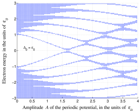
Figure 2: (Color online) Single electron spectrum in the potential (14) for the case $\Delta_{0}=\epsilon_{0}$.

The opposite regime is the strong coupling, or the tight-binding limit, in which case the external potential localizes the semi-classical Dirac electrons (holes) in its minima (maxima), tunneling between adjacent potential wells is exponentially suppressed, and minigaps become larger than the subbands. In this regime the wave function $u_{p}(x)$ becomes localized around the potential minimum, with its characteristic size

$${l_{\rm wf}}\ll\lambda_{\rm ext}\,.$$ (25)

The spectrum can be obtained by solving the problem (21) numerically via the transfer matrix. For an illustration, in Fig. 2 we plot the spectrum for the borderline case $\Delta_{0}=\epsilon_{0}$ in which the potential and kinetic energy in the Hamiltonian (20) are of the same order. Similar to the nearly free electron limit, the energy gaps oscillate as a function of $A$ and vanish at certain amplitude values. The spectrum also has a characteristic Dirac $\epsilon\to-\epsilon$ symmetry. Fig. 2 suggests that even for moderately strong backscattering $\Delta_{0}=\epsilon_{0}$ minigaps can occupy most of the spectrum when $A\sim\epsilon_{0}$.

In Appendix A we show that the limit (25) of exponentially suppressed interwell tunneling holds whenever

$$\left(\Delta_{0}\over\epsilon_{0}\right)^{-1}<{A\over\epsilon_{0}}<\left(\Delta_{0}\over\epsilon_{0}\right)^{c}\,,\quad\Delta_{0}>\epsilon_{0}\,,$$ (26)

where the exponent $c=3$ for tunneling from an energy level close to the bottom of the potential (or close to the top for holes), and $c=2$ for tunneling from a level far from the potential minimum or maximum.

Increasing the potential amplitude $A$ beyond $\Delta_{0}^{c}/\epsilon_{0}^{c-1}$ actually enhances the tunneling amplitude between the particle and hole continua. This is reflected in Fig. 2 by wider minibands for $A>\epsilon_{0}$. Indeed, an increase in $A$ makes the tunneling barrier through the Dirac gap $2\Delta_{0}$ shorter, and reduces the action under the barrier. The other way of understading the apparent delocalization of the wave functions for large $A$ is to notice that large potential amplitude results in strong oscillations of the potential term in Eq. (20). These oscillations effectively average this term to zero in the limit $A\to\infty$, in which case the minigaps become small as $A^{-1/2}$. The latter follows from the large–$A$ asymptotic behavior of the Bessel functions for the weak coupling minigaps (24) that become valid in this limit.

IV Bosonization

The Hamiltonian (3) is bosonizedStone ; Kane'97 ; Egger'97 ; Talyanskii'01 ; Levitov'01 by virtue of the massive Thirring — quantum sine-Gordon duality, Coleman ; Haldane by representing the fermionic operators (5) as nonlocal combinations of bose fields $\psi_{\alpha}\simeq(2\pi a)^{-1/2}\,e^{i\Theta_{\alpha}}$. The conjugate momenta

$$\Pi_{\alpha}={\hbar\over\pi v}\partial_{t}\Theta_{\alpha}$$ (27)

obey the canonical relations $\left[\Pi_{\alpha}(x),\,\Theta_{\beta}(y)\right]_{-}=-i\hbar\delta_{\alpha\beta}\,\delta(x-y).$ The result is the Lagrangian

$${\cal L} = {\frac{\hbar v}{2\pi}}\sum_{\alpha=1}^{4}\left(\frac{1}{v^{2}}\left(\partial_{t}\Theta_{\alpha}\right)^{2}-(\partial_{x}\Theta_{\alpha})^{2}-{2\Delta_{0}\over\hbar va}\cos 2\Theta_{\alpha}\right)$$ (28)

$$- \displaystyle{\frac{1}{2}}\int\!dx^{\prime}\,\rho(x)V(x-x^{\prime})\rho(x^{\prime})-\rho\left\{U(x)+\mu\right\}\,,$$

where the density $\rho(x)=\sum_{\alpha=1}^{4}\rho_{\alpha}=\sum_{\alpha=1}^{4}\textstyle{\frac{1}{\pi}}\,\partial_{x}\Theta_{\alpha}$, and $\mu$ is the chemical potential ($\mu=0$ at half-filling). The Gaussian part of the action is diagonalized by the combination of the unitary transformationTalyanskii'01 ; Levitov'01

$$\left(\matrix{\Theta_{1}\cr\Theta_{2}\cr\Theta_{3}\cr\Theta_{4}}\right)=\frac{1}{2}\left(\matrix{1&1&1&1\cr 1&-1&1&-1\cr 1&-1&-1&1\cr 1&1&-1&-1}\right)\left(\matrix{\theta^{0}\cr\theta^{1}\cr\theta^{2}\cr\theta^{3}}\right)$$ (29)

with the density (6) being a gradient of the charge mode $\theta^{0}$,

$$\rho(x)=\textstyle{\frac{2}{\pi}}\,\partial_{x}\theta^{0}\,,$$ (30)

and of the gauge transformation [cf. Eq. (17)]

$$\Theta_{\alpha}(x)\to\Theta_{\alpha}(x)-\textstyle\frac{1}{\hbar v}\int^{x}K^{-1}(U-\mu)\,dx^{\prime}$$ (31)

that leaves $\theta^{a}$ intact, and shifts

$$\theta^{0}\to\theta^{0}-\textstyle\frac{2}{\hbar v}\int^{x}K^{-1}(U-\mu)\,dx^{\prime}\,.$$ (32)

Here the charge stiffness

$$K_{q}=1+4\nu V(q)\,,\quad\nu={1\over\pi\hbar v}\,.$$ (33)

Below we drop the (irrelevant) logarithmic dependence of the stiffness $K_{q}$ on the momentum, assuming a constant value $K\!\equiv\!K_{q\sim 1/l_{\rm ch}}$, where $l_{\rm ch}\sim l_{s}$ is the charge soliton size (screening length for the Coulomb interaction). Using $e^{2}/\hbar v\simeq 2.7$ we estimate $K\simeq 40$ for $l_{\rm ch}\sim 1\,\mu$m for the stand-alone tube; $K\simeq 10$ for the tube placed on a substrate with a dielectric constant $\varepsilon=10$.

The nonlinear part of the action (28) is transformed using the identity $\sum_{\alpha=1}^{4}\cos 2\Theta_{\alpha}=4{\cal F}(\theta^{0},\theta^{a})$, where

$${\cal F}\left(\theta^{0},\,\theta^{a}\right)=\cos\theta^{0}\cdot\prod_{a=1}^{3}\cos\theta^{a}+\sin\theta^{0}\cdot\prod_{a=1}^{3}\sin\theta^{a},$$ (34)

yielding the Lagrangian Talyanskii'01 ; Levitov'01

$${\cal L}^{\prime}={\cal L}_{0}+{\cal L}_{\rm bs}\,,$$ (35)

$${\cal L}_{0} = {\hbar v\over 2\pi}\left\{\frac{1}{v^{2}}(\partial_{t}\theta^{0})^{2}-K\,(\partial_{x}\theta^{0})^{2}\right\}$$ (36)

$$+ {\hbar v\over 2\pi}\sum_{a=1}^{3}\left\{\frac{1}{v^{2}}(\partial_{t}\theta^{a})^{2}-(\partial_{x}\theta^{a})^{2}\right\},$$

$${\cal L}_{\rm bs} = -{\hbar vg_{0}\over\pi}{\cal F}(\theta^{0}+2\tilde{\mu}k_{\rm ext}x-2\tilde{A}\sin k_{\rm ext}x,\theta^{a}).\quad$$ (37)

The Lagrangian (35) describes one stiff charge mode $\theta^{0}$ and three soft flavor modes $\theta^{a}$, nonlinearly coupled by

$$g_{0}={4\Delta_{0}\over\hbar va}={4\over a^{2}}{\Delta_{0}\over D}\,,$$ (38)

where $D$ is the bandwidth (11), and the dimensionless quantities

$$\tilde{A}={A\over K\epsilon_{0}}\,,\quad\tilde{\mu}={\mu\over K\epsilon_{0}}$$ (39)

are introduced in a way similar to that of Eq. (18), with the energy scale $\epsilon_{0}$ defined in Eq. (19). The difference between Eqs. (39) and (18) is in the screening (by a factor of $1/K$) of external fields $U(x)$ and $\mu$ by the interacting NT system. When $g_{0}=0$, the electron number density (1) parametrized by $m$ varies continuously with $\tilde{\mu}$ as

$$m=2{\tilde{\mu}}\,.$$ (40)

In this case the system is a compressible scale-invariant Tomonaga-Luttinger liquid of the four flavors regardless of the electron interaction strength.FSA The nonlinear term (37) breaks charge-flavor separation by binding $\theta^{a}$ with $\theta^{0}$. It can become relevant at commensurate densities, yielding incompressible states.

Note that the Lagrangians (28) and (35) are SU(4) invariant, as is the original Hamiltonian ${\cal H}$. This invariance is not explicit in the adapted notation. It will manifest itself below on the level of renormalization.

V Phase soliton method

V.1 Electron as a composite soliton

Evaluation of excitation gaps requires the knowledge of how an added electron is represented in the language of the coupled bosonic fields (29). Here we first discuss this issue in a simpler case of a stand-alone tube, when no potential is applied: $U(x)\equiv 0$. We follow the framework of Levitov and Tsvelik,Levitov'01 emphasizing the details that will be important in the rest of the work.

The idea is that when interactions are strong ($K\gg 1$), the action (35) is dominated by the charge sector, which justifies optimization of (35) in a saddle point fashion, with $K^{1/2}$ playing the role of $\hbar^{-1}$. In particular, the soft neutral modes $\theta^{a}$ adjust themselves to provide an effective potential for the charged mode $\theta^{0}$ in such a way that the cost of adding charge is minimal. For the most part one can regard the charge mode as classical, since its quantum fluctuations are suppressed by $K^{-1/2}$ (and can be further included as corrections to the scaling laws as described in Sec. V.5 below), whereas the neutral fluctuations strongly renormalize the coupling (38), with its renormalized value $g$ given by Eq. (45) below.

As a result,Levitov'01 an electron added to a half-filled nanotube is a composite soliton characterized by the two length scales: the flavor $l_{\rm fl}$, and the charge $l_{\rm ch}\sim K^{1/2}l_{\rm fl}$, so that ${l_{\rm ch}}\gg{l_{\rm fl}}$. The neutral modes $\theta^{a}$ add a particular flavor to the electron, and, naturally, flavor is bound to charge by the non-linear term (37). Adding an electron of a given polarization $\alpha$ amounts to changing $\Theta_{\alpha}$ by $\pi$. According to the transformation (29), in the charge-flavor basis this results in a configuration in which all the fields $\theta^{0},\ \theta^{a}$ change by $\pm\pi/2$. However, given the separation of scales $l_{\rm ch}\gg l_{\rm fl}$, solitons of the flavor modes $\theta^{a}$ appear as sharp steps on the scale of $l_{\rm ch}$ that “switch” right in the middle of the charged soliton. The Coulomb interaction between electrons corresponds to overlap of charge soliton tails within the screening length ${l_{\rm ch}}$, whereas the fermionic exchange corresponds to overlap of the (shorter) flavor solitons. In the low-density regime $\bar{\rho}{l_{\rm fl}}\ll 1$, overlap of the charge-soliton tails maintans quasi-long-range order of a 1d Wigner crystal, whereas the effects of exchange are exponentially suppressed.

Technically, the effect of the neutral modes is to provide Fourier harmonics quadrupling in the nonlinear term (37), ${\cal F}(\theta^{0},\theta^{a})\to\bar{\cal F}(\theta^{0})\sim\cos 4\theta^{0}$. The optimization leading to the effective potential $\bar{\cal F}(\theta^{0})$ is shown in Fig. 3. On the classical level, minimizing ${\cal F}(\theta^{0},\theta^{a})$ over the values $\theta^{a}=n_{a}\pi/2$ with integer $n_{a}$ yields the potential

$$\bar{\cal F}_{\rm cl}(\theta^{0})=\min_{\{\theta^{a}=n_{a}\pi/2\}}{\cal F}(\theta^{a},\ \theta^{0})=\min\left\{\pm\cos\theta^{0},\ \pm\sin\theta^{0}\right\}$$ (41)

for the charge mode (top panel of Fig. 3). The switching between the branches of $\pm\cos\theta^{0}$ and $\pm\sin\theta^{0}$ occurs via the neutral fields changing by $\pm\pi/2$ right in the middle of the slow charge soliton, when $\theta^{0}$ has changed by $\pi/4$. One obtains the classical soliton of the charge mode of the formLevitov'01

$$\theta_{\rm cl}^{0}(x)=\left\{\matrix{2\cos^{-1}\tanh(u-x/l_{\rm ch}^{(\rm cl)})\,,&x<0\,,\cr\frac{\pi}{2}-2\cos^{-1}\tanh(u+x/l_{\rm ch}^{(\rm cl)})\,,&x>0\,,}\right.$$ (42)

where $l_{\rm ch}^{(\rm cl)}=(K/g)^{1/2}$ and $\tanh u=\cos\pi/8$.

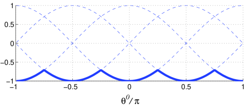
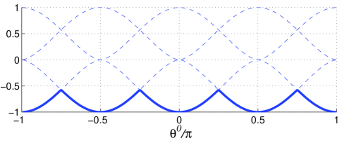
Figure 3: (Color online) Classical $\bar{\cal F}_{\rm cl}(\theta^{0})$ (top) and renormalized $\bar{\cal F}(\theta^{0})$ (bottom) effective potentials (shown in bold) for the charge mode in the case of $K\gg 1$, Eqs. (41) and (44)

Quantum fluctuations of the neutral sector renormalize the bare potential $\sim g_{0}\bar{\cal F}_{\rm cl}(\theta^{0})$ by providing it with the scaling dimension

$$\gamma=8/5\,.$$ (43)

As a result, the effective potential for the charge sector

$$\matrix{{\cal L}_{\rm bs}\to-\left({\hbar v\over\pi}\right)V_{\rm charge}\,,\quad V_{\rm charge}=g\bar{\cal F}(\theta^{0})\,,\cr\bar{\cal F}(\theta^{0})=-\left[-\bar{\cal F}_{\rm cl}(\theta^{0})\right]^{\gamma}\,,}$$ (44)

where the renormalized nonlinear coupling

$$g\simeq\frac{1}{a^{2}}\left({\Delta_{0}\over D}\right)^{\gamma}\,,$$ (45)

and the cutoff $D$ defined in Eq. (11). The potential $\bar{\cal F}(\theta^{0})$ is plotted in the lower panel of Fig. 3. The result (44) is justified in the adiabatic approximation ${l_{\rm ch}}\gg{l_{\rm fl}}$ when the potential (41) is slow on the scale $a<l<{l_{\rm fl}}$ on which quantum fluctuations of the fields $\theta^{a}$ accumulate (for renormalization procedure see Sec. V.5 below).

Although the difference between the form of the potential (41) [considered in Ref. Levitov'01, ], and the renormalized one, $\bar{\cal F}(\theta^{0})$ [Eq. (44)], is not crucial qualitatively,Novikov-unpub it can be important for quantitative considerations. Namely, it affects both the soliton energy, its size, ${l_{\rm fl}}$, and the effective screening length, ${l_{\rm ch}}$. Unfortunately, the analytic form for the charge mode soliton with the potential term (44) is unavailable. One way to find this soliton is to approximate the potential (44) by a piecewise-quadratic function [this procedure works wellLevitov'01 for the soliton in the nonrenormalized potential (41)]. This yields

$$\theta^{0}(x)\approx\theta_{\rm quad}^{0}(x)=\left\{\matrix{\frac{\pi}{4}e^{x/{l_{\rm ch}}}\,,&x<0\,,\cr\frac{\pi}{2}-\frac{\pi}{4}e^{-x/{l_{\rm ch}}}\,,&x>0\,,}\right.$$ (46)

with a charge soliton size

$${l_{\rm ch}}=\left({K/\gamma g}\right)^{1/2}\,,$$ (47)

which is a factor $\approx 1.26$ shorter compared to that in Eq. (42).

Physically, strong Coulomb repulsion in the presence of the curvature $\Delta_{0}$ of electronic dispersion qualitatively changes the conventional “spin-flavor separated” Luttinger-liquid behavior governed by the Gaussian action (36). At the Luttinger fixed point, all the modes enter on equal footing, and the dispersion curvature is irrelevant at high density. At low density, the saddle point of the total action (35) describes the crossover to the Wigner crystal, in which flavor is bound to charge. The neutral and the charge sectors play very different roles in the Wigner crystal regime: the former creates the effective potential for the latter. This effective potential (44) has a period $\pi/2$ that is four times smaller than that of the potential (37) with fixed $\theta^{a}$; the lowest harmonic in the Fourier expansion

$$\bar{\cal F}(\theta^{0})={\rm const}-\sum_{n=1}^{\infty}f_{n}\cos(4n\theta^{0})$$ (48)

is $\cos 4\theta^{0}$. The purpose of this period reduction is to lower the Coulomb energy by splitting the $\theta^{0}\to\theta^{0}+2\pi$ excitation that carries charge $4e$ [according to Eq. (30)] and is a flavor singlet, into four subsequent excitations each carrying a single fermion of a unit charge and of a particular flavor.

Practically, to obtain a smooth approximate form of the charge soliton, and to estimate its energy that dominates the cost of adding an electron, here we keep the most relevant harmonic in the Fourier series (48),

$$\bar{\cal F}(\theta^{0})\approx-f_{1}\cos 4\theta^{0}\,,\quad f_{1}\approx 0.178\,.$$ (49)

The approximation (49) overestimates the classical charge soliton energy by 10%:

$$E_{\rm ch.sol.}^{\rm approx.}=c_{1}{\hbar v\over\pi}\sqrt{Kg}\,,\quad c_{1}=\sqrt{4f_{1}}\approx 0.844\,,$$ (50)

compared with the energy in the full potential (44):

$$E_{\rm ch.sol.} = c_{\infty}{\hbar v\over\pi}\sqrt{Kg}\,,$$ (51)

$$c_{\infty} = \sqrt{8}\int_{0}^{\pi/4}\!d\theta^{0}\,\sqrt{1-\cos^{\gamma}\theta^{0}}\approx 0.752\,.$$

The charge soliton in the potential (49) takes the form

$$\theta^{0}_{\rm approx}(x)=\textstyle{\frac{1}{2}}\cos^{-1}\tanh(-x/{l_{\rm ch}}^{\prime})$$ (52)

with the rescaled size ${l_{\rm ch}}^{\prime}=\frac{1}{4}(K/f_{1}g)^{1/2}\approx l_{\rm ch}^{\rm(cl)}/1.69$. Note that, due to strong renormalization by the neutral fluctuations, the potential (44) is steeper than its classical counterpart (41). This leads to shorter charge soliton length than that of a classical solution (42), as both of the approximations, Eqs. (46) and (52), indicate.

Remarkably, the difference between the Luttinger liquid [described by the Gaussian Lagrangian (36)], and the Wigner crystal will become crucial after adding the external potential $U(x)$. Depending on the relation between its period, $\lambda_{\rm ext}$, and the “size of an electron”, ${l_{\rm fl}}$, either the Gaussian saddle point ($g_{0}\to 0$) of the action (35), or the Wigner-crystal saddle point described above will play out. The latter one applies in the regime $\lambda_{\rm ext}\gg{l_{\rm fl}}$ considered below in Section VII. There we show that the system effectively behaves as that of a single mode.

V.2 Incompressible states of the classical bosonic fields

The above discussion of the transition to the Wigner crystal suggests that, already on the classical level, the nonlinear action (28) or (35) captures important physics even on the short length scale (smaller than the inter-particle distance!). This intuition can be readily extended onto the $U\neq 0$ case. By adding the external potential (14), below we use the classical Hamiltonian

$$\matrix{{\cal H}_{\rm cl}[\Theta_{\alpha}]=\displaystyle{1\over 2}\sum(\partial_{x}\Theta_{\alpha})^{2}+\displaystyle{{K-1\over 8}}\,\left(\sum\partial_{x}\Theta_{\alpha}\right)^{2}\cr+\frac{1}{4}g_{0}\sum\cos 2\Theta_{\alpha}+\displaystyle{\frac{1}{\hbar v}}\,\sum\partial_{x}\Theta_{\alpha}\cdot\left({U(x)}\!-\!\mu\vphantom{1^{2^{3}}}\right),}$$ (53)

that follows from the Lagrangian (28), to numerically illustrate how incompressible states appear. For convenience here we work in the original basis $\Theta_{\alpha}$.

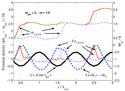
Figure 4: (Color online) Classical ground state of the Hamiltonian (53) for the density $m=1/2$. Bold solid line marks the external potential. Fine lines in the upper part denote the solitons of the fields $\Theta_{\alpha}$ found by the numerical minimization of Eq. (53) for $\tilde{\mu}=1/4$, $K=10$, $g_{0}=12k_{\rm ext}^{2}$, $A=K\epsilon_{0}$. The corresponding fine lines in the lower part denote the flavor densities $\delta\rho_{\alpha}=\rho_{\alpha}-m/\lambda_{\rm ext}$ counted from their average value $m/\lambda_{\rm ext}$. Bold dashed line is the total density counted from its average value $4m/\lambda_{\rm ext}$. Note the period doubling for $\Theta_{\alpha}(x)$.

Consider the simplest fractional density, $m=1/2$, corresponding to the chemical potential $\tilde{\mu}=1/4$ [cf. Eq. (40)]. Its classical ground state is an incompressible configuration in which the solitons of the fields $\Theta_{\alpha}$ occupy every other potential minimum, as shown in Fig. 4. This Figure is a result of the numerical minimization of the Hamiltonian (53) with respect to the fields $\Theta_{\alpha}$. In agreement with the general theoryPokrovsky (developed for a single-mode system), for the fraction $m=p/q$ the density should have the period $q\lambda_{\rm ext}$. In our case of the four modes, naturally, the period of the density $\frac{1}{\pi}\partial_{x}\Theta_{\alpha}$ in each mode is $q\lambda_{\rm ext}$, with $q=2$ in Fig. 4. Note that, since the total density $m_{\rm tot}=2$ is integer, the charge density period coincides with that of $U(x)$. In the absence of $U(x)$, all the solitons of $\Theta_{\alpha}$ would be equally separated from each other due to the Coulomb repulsion. The finite$-U$ configuration shown in Fig. 4 is the result of an interplay between the mutually repelling solitons and a confining periodic potential. We note that the fermionic exchange of the original problem (3) is manifest here already on the classical level, in the fact that solitons of the same flavor repel each other stronger, and, therefore, do not occupy the adjacent potential minima.

V.3 Phase soliton method for a single mode

To systematically study excitation gaps over commensurate configurations, we employ and generalize the phase soliton method. Representing an excitation in a commensurate phase by a phase soliton was utilized in the past in various contexts. The model of locking a system into a commensurate state was first suggested in the work of Frenkel and Kontorova.Frenkel Later, it was re-discovered and solved by Frank and van der Merwe FvdM in the context of atoms ordering on crystal surfaces, and by Dzyaloshinskii Dzyal describing a transition to the state with a helical magnetic structure. The general theory of commensurate-incommensurate phase transitions has been finalized by Pokrovsky and Talapov.Pokrovsky The result of these investigations is a finite or infinite sequence of gaps (“devil’s staircase”) corresponding to commensurate states. Bak

The essense of the phase soliton method can be demonstrated on the example of the single-mode system. Consider the model Hamiltonian of the form

$${\cal H}_{1}=\frac{K}{2}(\partial_{x}\theta)^{2}+g\cos(\beta\theta+mk_{\rm ext}x+b\sin k_{\rm ext}x)$$ (54)

[cf. Eqs. (28), (35), or (53), albeit with only one mode present]. To make contact with the nanotube system, the parameters in the Hamiltonian (54) have a similar meaning to those in the action (28) transformed by (31), with $\beta=2$ and only $\Theta_{1}$ present. The Hamiltonian (54) is the continuous form of the Frenkel-Kontorova modelFrenkel that describes locking of the compressible lattice of interacting particles (e.g. a chain of atoms) by the external potential of the period $\lambda_{\rm ext}$ (e.g. the substrate potential for the atomic chain), as is schematically shown in Fig. 1(a). The phase field $\theta$ represents the deviations from equilibrium positions along the chain, with changing $\theta$ by $2\pi/\beta$ corresponding to a shift of the chain by its period. The gradient $\beta\partial_{x}\theta/2\pi$ thus has a meaning of the excess particle density near point $x$. The coupling between the particles and the potential is represented by $g$, whereas the lowest harmonic of the potential is $\propto b\cos k_{\rm ext}x$. The crucial parameter is the period ratio $m$ (number of particles per period $\lambda_{\rm ext}$).

External potential can lock the chain into incompressible states when $m$ is either an integer, or a simple fraction $m=p/q$. An excitation (an incommensuration) over such a commensurate state corresponds to adding an extra particle to the system. This changes the positions of other particles in the chain due to their mutual interaction. When the coupling $g$ is small, such a change occurs over many periods $\lambda_{\rm ext}$ [as illustrated in Fig. 1(c)].

In the language of the continuous model (54), the incommensuration is represented by the soliton-like change of $\theta$ by $2\pi/\beta$, with the excitation gap given by the soliton energy. The effective theory for the excitation follows from the Euler-Lagrange equation for (54), $\delta{\cal H}_{1}/\delta\theta=0$, practically found by expanding in the powers of $g$,

$$\theta=\bar{\theta}+{\theta}^{(1)}+...+{\theta}^{(n)}+...\,,\quad\theta^{(n)}={\cal O}(g^{n})\,.$$ (55)

Here $\bar{\theta}$ is constant in the commensurate phase, acquiring a slow coordinate dependence $\bar{\theta}(x)$ in an excitation (phase soliton). When $m$ is integer, the zeroth order term $\theta=\bar{\theta}$ in the expansion (55) is enough: Averaging over a period $\lambda_{\rm ext}$, the effective Hamiltonian is $K(\partial_{x}\bar{\theta})^{2}/2+gJ_{m}(b)\cos\beta\bar{\theta}$, and the excitation is described by the sine-Gordon soliton of a slow mode $\bar{\theta}(x)$ that interpolates by $2\pi/\beta$ over a few $\lambda_{\rm ext}$.

For the fractional density $m=p/q$, averaging $g\cos(\beta\bar{\theta}+mk_{\rm ext}x+b\sin k_{\rm ext}x)$ over $q\lambda_{\rm ext}$ gives zero for constant $\bar{\theta}$. This indicates that the effective potential for $\bar{\theta}$ is of the higher order in the coupling $g$. Using the expansion (55), one obtains the lowest order Hamiltonian for the phase soliton $\bar{\theta}(x)$ of the form $K(\partial_{x}\bar{\theta})^{2}/2+g_{q}(b)\cos\beta q\bar{\theta}$, $g_{q}\sim g^{q}$. The corresponding soliton energy estimates the excitation gap. One also has to average over the thermal or quantum fluctuations to assess the relevance of the potential term $\sim\cos\beta q\bar{\theta}$, in which case the (omitted) overall coefficient in front of the Hamiltonian (54) becomes important, as it controls the size of fluctuations.

V.4 Phase soliton method for a nanotube

Below we show that the case of multiple modes is qualitatively different from a conventional single mode situation described above. This difference manifests itself in the presence of the two regimes of coupling of the NT electron system to the external potential. Physically, the choice of the regime depends on whether the electron wavefunctions overlap with each other substantially, — that is, whether the physics is determined by the quantum interference with fermionic exchange being important, or by the Coulomb repulsion between nearly point-like electrons, in which case the exchange effects are negligible.

Technically, the difference between the regime of Bragg diffraction in a Luttinger liquid (“weak coupling”), or of pinning of the Wigner crystal (“strong coupling”) is determined by the saddle point of the nonlinear action (35). In particular, if the neutral modes switch fast on the scale on which the argument of the potential (37) changes appreciably, the Wigner-crystal saddle point (Sec. V.1) is selected, and the system is described in terms of the single (charge) mode, with the problem reduced to that described in Sec. V.3 above. If, on the other hand, the neutral modes are slow, the weak-coupling saddle point (expansion around $g_{0}=0$) is the relevant one.

To define the regimes of coupling we need to compare the size $\bar{l_{\rm fl}}$ of the phase soliton $\bar{\theta}^{a}(x)$ of the flavor sector (size of the added electron) with the potential period $\lambda_{\rm ext}$. For now, we assume that $\bar{l_{\rm fl}}$ is known. The scale $\bar{l_{\rm fl}}$ will be later obtained self-consistently as a result of integrating over the quantum fluctuations (performed for different cases in Sections V.5, VI and VII).

Weak coupling

In the weak coupling regime the flavor soliton tails, which correspond to fermions of the same flavor, overlap. Physically, it means that the system “knows” that it is composed of the particles of different flavors since the role of exchange is important. An extreme example of this regime is a non-interacting system in which fermions of the same flavor effectively repel due to the Pauli principle, whereas fermions of different flavors do not notice each other.

Strong overlap between the soliton tails in a commensurate configuration requires large ${l_{\rm fl}}\gg\lambda_{\rm ext}$, or, equivalently, small coupling $g_{0}$ in Eq. (35). The system is close to the Luttinger liquid, i.e. it is compressible for almost all densities apart from a few commensurate ones, for which small minigaps open up. This regime has been considered in Ref. Talyanskii'01, for integer $m$. The smallness of $g_{0}$ warrants finding the effective Lagrangian

$${\cal L}_{m}[\bar{\theta}^{0},\bar{\theta}^{a}]={\cal L}_{0}[\bar{\theta}^{0},\bar{\theta}^{a}]+{\cal L}_{m}^{\rm int}[\bar{\theta}^{0},\bar{\theta}^{a}]$$ (56)

for the phase modes $\bar{\theta}^{0}$ and $\bar{\theta}^{a}$ perturbatively in $g_{0}$ (similarly to the single-mode model case considered in Sec. V.3 above), treating all the modes on equal footing. Namely, from the Lagrangian (35) with the chemical potential (40) corresponding to the commensurate density (1) parametrized by $m=p/q$, one finds the effective potential ${\cal L}_{m}^{\rm int}[\bar{\theta}^{0},\bar{\theta}^{a}]$ for the phase modes to the lowest order in $g_{0}$ by solving the time-independent Euler-Lagrange equations $\delta{\cal L}^{\prime}/\delta\theta^{0}=0$ and $\delta{\cal L}^{\prime}/\delta\theta^{a}=0$, via the expansion

$$\matrix{\theta^{0}=\bar{\theta}^{0}+{\theta^{0}}^{(1)}+...+{\theta^{0}}^{(n)}+...\,,\cr\theta^{a}=\bar{\theta}^{a}+{\theta^{a}}^{(1)}+...+{\theta^{a}}^{(n)}+...\,,\cr{\theta^{0}}^{(n)}={\cal O}(g_{0}^{n})\,,\quad{\theta^{a}}^{(n)}={\cal O}(g_{0}^{n})\,.}$$ (57)

The first term in (56) is the Gaussian Lagrangian (36) as a function of the slow phase modes, and the obtained potential energy ${\cal L}_{m}^{\rm int}$ is of the order $g_{0}^{q}$ (before integrating over quantum fluctuations).

From the Lagrangian ${\cal L}_{m}[\bar{\theta}^{0},\bar{\theta}^{a}]$ one finds the commensurate ground state in which the phase modes $\bar{\theta}^{0}$ and $\bar{\theta}^{a}$ are constant. Similarly to the electron added to a stand-alone tube being represented by a composite soliton (Sec. V.1), an excitation over such a ground state is a composite phase soliton of the slow phase modes $\bar{\theta}^{0}(x),\ \bar{\theta}^{a}(x)$. It can be found as a saddle point of the Lagrangian ${\cal L}_{m}[\bar{\theta}^{0},\bar{\theta}^{a}]$ in a way similar to that described above in Sec. V.1.

The weak coupling limit is illustrated below by considering the simplest situation of integer density $m$, in which case the decomposition (57) is trivial since it contains just one term for each mode. Hence ${\cal L}_{m}[\bar{\theta}^{0},\bar{\theta}^{a}]$ is precisely the Lagrangian (35) written as a function of $\theta^{0,a}=\bar{\theta}^{0,a}$ with the chemical potential $\tilde{\mu}$ given by Eq. (40).

Technically, the weak coupling regime is characterized by the slow “switching” of the flavor modes $\theta^{a}$ on the scale on which the phase of the charge part of the potential energy ${\cal L}_{m}^{\rm int}[\bar{\theta}^{0},\,\bar{\theta}^{a}]$ in the Lagrangian (56) changes by $2\pi$. For integer $m$, the potential energy is just the nonlinear term (37) written as a function of the slow modes $\bar{\theta}^{0},\,\bar{\theta}^{a}$. Thus we demand

$$\matrix{m{l_{\rm fl}}\gg\lambda_{\rm ext}\,,\cr 2\tilde{A}\sin k_{\rm ext}{l_{\rm fl}}\gg 2\pi\,.}$$ (58)

The first condition in Eq. (58) requires the flavor excitation to be extended on the scale of the separation $4\bar{\rho}^{-1}=\lambda_{\rm ext}/m$ between same-flavor fermions. The meaning of the second condition will be made more clear below. The weak coupling limit (58) results in the following approximation for the energy (37):

$$\matrix{{\cal F}(\bar{\theta}^{0}+mk_{\rm ext}x-2\tilde{A}\sin k_{\rm ext}x,\ \bar{\theta}^{a})\cr\approx J_{m}(2\tilde{A}){\cal F}\left(\bar{\theta}^{0},\ \bar{\theta}^{a}\right)\to J_{m}(2\tilde{A})\bar{\cal F}_{\rm cl}(\bar{\theta}^{0})\,.}$$ (59)

Here we discarded spatially oscillating terms (in other words, we averaged ${\cal F}$ over the period $\lambda_{\rm ext}$), and denoted by the arrow the soft mode “switching” that produced the optimized potential (41).

The procedure (59) as written is allowed for the integer density $m$. In the case when the density $m=p/q$ is a simple fraction one needs to utilize the phase soliton approach to find the effective potential of order $g_{0}^{q}$ and then perform analogous optimization. The weak coupling limit is considered in Sec. VI.1 for integer $m$ and in Sec. VI.2 for the simplest fractional density $m=1/2$.

Strong coupling

In the opposite, strong coupling limit, the Coulomb interaction wins over the effects of the fermionic exchange. In this regime the system “forgets” its four-flavor nature, and effectively behaves as that of spinless Dirac fermions with the total density (1). Technically, the soft mode “switching” (denoted by the arrow below) occurs before averaging over the period of the potential,

$${\cal F}\left(\bar{\theta}^{0}+mk_{\rm ext}x-2\tilde{A}\sin k_{\rm ext}x,\ \bar{\theta}^{a}\right)$$

$$\to\bar{\cal F}\left(\bar{\theta}^{0}+mk_{\rm ext}x-2\tilde{A}\sin k_{\rm ext}x\right)$$

$$=f_{1}\cos\left(4\bar{\theta}^{0}+m_{\rm tot}k_{\rm ext}x-8\tilde{A}\sin k_{\rm ext}x\right)$$

$$+f_{2}\cos\left(8\bar{\theta}^{0}+2m_{\rm tot}k_{\rm ext}x-16\tilde{A}\sin k_{\rm ext}x\right)+...$$

$$\approx f_{1}\cos\left(4\bar{\theta}^{0}+m_{\rm tot}k_{\rm ext}x-8\tilde{A}\sin k_{\rm ext}x\right)\,.$$ (60)

Here the Fourier coefficients $f_{n}$ are defined in Eq. (48), and in the last line we used the approximation (49). Note the dependence of the resulting potential energy on the total density $m_{\rm tot}=4m$. The condition for the saddle point (60) is

$$\matrix{m{l_{\rm fl}}<\lambda_{\rm ext}\,,\cr 2\tilde{A}\sin k_{\rm ext}{l_{\rm fl}}<2\pi\,.}$$ (61)

This regime is considered below in Section VII.

Now let us clarify the meaning of the second condition in Eqs. (58) and (61). Increasing the potential amplitude $A$ much beyond $K\hbar v/{l_{\rm fl}}$ effectively averages out the nonlinear term and thus draws the system into the weak coupling limit (58). This situation is similar to the noninteracting case considered in Section III above, where the approximation (24) becomes valid at large $A$.

To summarize, above we have generalized the phase soliton method to the multiple-mode case. After the appropriate effective action for the slow modes is chosen [either Eq. (56), or the one based on the potential energy (60)], excitations are described by the corresponding phase solitons. Due to the electron-hole symmetry of the original problem, adding an electron to a commensurate state (phase soliton) costs the same energy $\Delta_{m}$ as removing an electron from the same state (anti-soliton), while the sum of the two energies, $2\Delta_{m}$, is the corresponding excitation gap.

V.5 Effect of quantum fluctuations

To illustrate integration over quantum fluctuations, below we renormalize the gap $\Delta_{0}$ for the stand-alone tube. (Generalizations for the $U\neq 0$ will be made in subsequent Sections.) Fluctuations of the neutral sector around the saddle point described in Sec. V.1 above are governed by the Lagrangian (35) with fixed value of $\theta^{0}$. Adiabaticity of the charged mode at $K\gg 1$ ensures that $\theta^{0}\simeq{\rm const}$ on the length scales $a<l<{l_{\rm fl}}$ where quantum fluctuations of the flavor sector accumulate. With each neutral field contributing to the scaling dimension by 1/4, flavor fluctuations result in the scaling dimension

$$\gamma_{0}=3/4$$ (62)

for the adiabatic charge mode potential (41), yielding

$$V_{\rm charge}(l)=V_{\rm charge}(a)\left({l\over a}\right)^{-\gamma_{0}},\quad V_{\rm charge}(a)=g_{0}\bar{\cal F}_{\rm cl}(\theta^{0})\,,$$ (63)

where $l$ is the renormalization-group (RG) scale, and $a$ is the tube radius. Since $\gamma_{0}<2$, the potential $V_{\rm charge}$ is relevant and grows. The flow (63) stops on the scale $l\simeq{l_{\rm fl}}$ on which the potential energy becomes comparable to the kinetic energy of the flavor sector, since the perturbative RG yields the law (63) only while the renormalized coupling stays small.CallanSymanzik For the larger scales $l>{l_{\rm fl}}$ the potential energy dominates and the problem becomes classical.

The scale ${l_{\rm fl}}$ has a twofold meaning. First, it is the correlation length for the flavor, estimated self-consistently from the balance of kinetic and potential terms

$$V_{\rm charge}({l_{\rm fl}})\simeq{1\over{l_{\rm fl}}^{2}}\,.$$ (64)

Beyond $x\simeq{l_{\rm fl}}$ the correlation functions of the $\theta^{a}$ fields decay exponentially, rather than in a power-law fashion. From Eqs. (63) and (64) we obtain the renormalized potential (44) for the charge mode with the coupling (45) and the scaling exponent (43),

$$\gamma={2\over 2-\gamma_{0}}\,.$$ (65)

The second meaning of the scale ${l_{\rm fl}}$ is the renormalized size of the flavor soliton of the model (35) with fixed $\theta^{0}$.

Since the charge sector is stiff, the excitation gap $\Delta$ is dominated by the charge soliton energy. The latter can be now estimated classically [cf. Eq. (50)] from the effective charge mode Lagrangian

$${\cal L}_{\rm charge}=\displaystyle{\hbar v\over\pi}\left(\frac{1}{2v^{2}}(\partial_{t}\theta^{0})^{2}-\frac{K}{2}(\partial_{x}\theta^{0})^{2}-V_{\rm charge}\right)$$

$$\approx\displaystyle{\hbar v\over\pi}\left(\frac{1}{2v^{2}}(\partial_{t}\theta^{0})^{2}-\frac{K}{2}(\partial_{x}\theta^{0})^{2}-gf_{1}\cos 4\theta^{0}\right),$$ (66)

where we used the saddle point approximation (44), (45) and (49) outlined in Sec. V.1 above. In the limit $K\to\infty$ the effective Lagrangian (66) yields the gapTalyanskii'01 ; Levitov'01

$$\Delta_{K\to\infty}\simeq K^{1/2}D^{1/5}\Delta_{0}^{4/5}\,.$$ (67)

At finite $K$ the problem of finding exact scaling laws in the nonlinear theory (35) is far from trivial. Here we attempt to estimate the ${\cal O}(\eta)$ corrections,

$$\eta=K^{-1/2}\,,$$ (68)

to the $K=\infty$ scaling laws in Eq. (67). For that we note that in one-loop RG, one averages the nonlinear term ${\cal L}_{\rm bs}$ over the independent Gaussian fluctuations described by the Gaussian action ${\cal L}_{0}$ diagonal in charge and flavor. Due to the factorization (34), the result of such an averaging can be represented in the form of the product of the contributions of independent Gaussian theories, with the terms of the action (35) scaling as

$${K\over{l_{\rm ch}}^{2}}+{1\over{l_{\rm fl}}^{2}}+g_{0}\left({{l_{\rm fl}}\over a}\right)^{-\gamma_{0}}\left({{l_{\rm ch}}\over a}\right)^{-\eta/4}.$$ (69)

Minimizing the composite-soliton action of the form (69) over both ${l_{\rm ch}}$ and ${l_{\rm fl}}$ amounts to including the coupling between the flavor and charge fluctuations by the nonlinear term. The variational estimate yields

$${{l_{\rm fl}}\over a}\simeq K^{\zeta}\left({D\over\Delta_{0}}\right)^{4\over 5-\eta},\quad{l_{\rm ch}}\simeq K^{\frac{1}{2}}{l_{\rm fl}}\,,\quad\textstyle{\zeta={\eta\over 10-2\eta}}$$ (70)

for the correlation lengths, and produces the renormalized gap $\Delta\simeq\hbar vK/{l_{\rm ch}}$ that scales as

$$\Delta\simeq K^{\frac{1}{2}-\zeta}D^{\frac{1-\eta}{5-\eta}}\Delta_{0}^{\frac{4}{5-\eta}}\,.$$ (71)

The latter expression smoothly crosses over to the noninteracting case $K=1$, $\Delta=\Delta_{0}$, and it also has a correct scaling (67) in the classical limit $K\to\infty$.compare-LT

VI Weak coupling limit

VI.1 Integer density $m=\pm 1,\pm 2,...$

The saddle point (59) maps the problem of finding excitation gaps onto that with $U\equiv 0$ and

$$g_{0}\to g_{m}\simeq g_{0}J_{m}(2\tilde{A})\,.$$ (72)

Based on the results of Sections V.1 and V.5, one obtains the renormalized minigaps $2\Delta_{m}$, where

$$\Delta_{m}\simeq K^{1/2-\zeta}D^{{1-\eta\over 5-\eta}}\left(\Delta_{m}^{(0)}(\tilde{A})\right)^{4\over 5-\eta}$$ (73)

[cf. Eq. (71)], and where the bare minigaps

$$\Delta_{m}^{(0)}(\tilde{A})=\Delta_{0}\,|J_{m}(2\tilde{A})|$$ (74)

given by their noninteracting values (24) with the screened potential amplitude $\tilde{A}$ defined in Eq. (39). Eq. (73) in the $K\to\infty$ limit corresponds to minigaps found in Ref. Talyanskii'01, . The qualitative features of the noninteracting minigaps (24) persist in the interacting case.Talyanskii'01 Namely, as a function of the screened potential amplitude (39), the minigaps (73) oscillate, vanishing at particular values of $\tilde{A}$. However, minigaps (73) are strongly enhanced in magnitude compared to (24) due to electron interactions. Also the dependence of the minigaps on both the bare backscattering $\Delta_{0}$ and on the periodic potential amplitude $A$ has a characteristic power law behavior which, in the limit of strong interactions $K\gg 1$, is given by a universal power law $4/5$ characteristic of the number of NT fermion polarizations at half-filling.

What is the cost of adding electron’s flavor on top of its charge? According to the mapping (72), the problem is formally equivalent to that with $U\equiv 0$, so the results of Ref. Levitov'01, apply: On the energy scale below that of the frozen charge sector, the flavor sector is governed by the effective SU(4)$\simeq$O(6) Gross-Neveu LagrangianLevitov'01 ; GN

$${\cal L}_{\rm GN} = {\hbar v\over\pi}\int\!dx\left\{\frac{1}{2}(\partial_{\mu}\theta^{a})^{2}-g_{\rm GN}\sum_{a>b}\cos 2\theta^{a}\cos 2\theta^{b}\right\}$$ (75)

$$= \hbar v\int\!dx\left\{i\bar{\chi}_{j}\gamma_{\mu}\partial_{\mu}\chi_{j}-g_{\rm GN}(\bar{\chi}_{j}\chi_{j})(\bar{\chi}_{j^{\prime}}\chi_{j^{\prime}})\right\},$$

where $\chi_{j}$ are the Majorana fermions and the Gross-Neveu coupling in our case is $g_{\rm GN}\propto g_{m}$. The excitations of the model (75) are massive relativistic particles transforming according to different representations of the O(6) group,Z with the mass scale physically originating due to effects of exchange.

VI.2 Fractional density $m=\frac{1}{2}$

Using the phase soliton method outlined in Sec. V.3 above, we derive the effective phase mode Lagrangian

$${\cal L}_{1/2}[\bar{\theta}^{0},\bar{\theta}^{a}]={\cal L}_{0}[\bar{\theta}^{0},\bar{\theta}^{a}]+{\cal L}_{1/2}^{\rm int}[\bar{\theta}^{0},\bar{\theta}^{a}]$$ (76)

given by the sum of the Gaussian part ${\cal L}_{0}$ [Eq. (36)] and the potential energy [see Appendix B for details]

$$-{\cal L}_{1/2}^{\rm int} = {\hbar vg_{0}^{\prime}\over 4\pi}\left\{\vphantom{\sum_{a}^{3}}(4-\kappa)v_{1/2}(2\tilde{A}){\cal F}(2\bar{\theta}^{0},\,2\bar{\theta}^{a})\right.$$ (77)

$$\left.-\kappa v_{1/2}(2\tilde{A})\sum_{a}\cos 2\bar{\theta}^{a}\cos 2\bar{\theta}^{0}\right.$$

$$\left.+\kappa u_{1/2}(2\tilde{A})\sum_{a>b}\cos 2\bar{\theta}^{a}\cos 2\bar{\theta}^{b}\right\}.\quad$$

Here the function ${\cal F}$ is defined in Eq. (34) and the other quantities are defined in Appendix B.

Let us discuss the potential energy (77). Its first term has scaling dimension 3 and is irrelevant. The second term of the potential (77) is responsible for the charge excitation gap $\Delta_{\rm ch,1/2}$. In the limit $K\gg 1$, this term has scaling dimension

$$\gamma_{1/2}=1$$ (78)

and grows under the renormalization group flow. Finally, the third term is marginal. It describes the SU(4) flavor physics on the energy scale $\Delta_{\rm fl}\sim K^{-1/2}\Delta_{\rm ch,1/2}$.

The charge gap is found via the saddle-point optimization of the second term of the potential (77) by the neutral sector in a way similar to that of Sec. V.1 above. Adding an extra electron to the system (76) corresponds to a composite phase soliton in which the $\bar{\theta}^{a}$ fields “switch” by $\pi/2$ in the middle of a slow charged phase soliton, at the point when $\cos 2\bar{\theta}^{0}=0$. (It is possible to showNovikov-unpub that although at this very point the effective sine-Gordon coupling $\propto\cos 2\bar{\theta}^{0}$ for the neutral sector vanishes, the flavor soliton has a finite size and energy. This is the case since away from the center of the charged soliton, $\cos 2\bar{\theta}^{0}\neq 0$ giving the finite flavor scale.)

On the classical level, the neutral sector produces the charge potential $\bar{\cal F}_{\rm cl}^{(1/2)}$ [top panel of Fig. 5],

$$\sum_{a}\cos 2\bar{\theta}^{0}\cos 2\bar{\theta}^{a}\to\bar{\cal F}_{\rm cl}^{(1/2)}(\bar{\theta}^{0})=-\left|\cos 2\bar{\theta}^{0}\right|\,.$$ (79)

By integrating over the flavor fluctuations we obtain the flow of the form (63) with the scaling exponent (78) for the potential energy $g_{1/2}\bar{\cal F}_{\rm cl}^{(1/2)}(\bar{\theta}^{0})$, where

$$g_{1/2}=\textstyle{\frac{1}{4}}\kappa g_{0}^{\prime}|v_{1/2}(2\tilde{A})|\,.$$ (80)

From the self-consistency of the form (64) we find the flavor scale

$${l_{\rm fl}}_{,1/2}\sim{a\over\kappa|v_{1/2}(2\tilde{A})|}\left({\epsilon_{0}\over\Delta_{0}}\right)^{2},$$ (81)

[$a$ is the tube radius], the renormalized coupling

$$g_{1/2}^{*}\simeq{1\over{l_{\rm fl}}_{,1/2}^{2}}\propto g_{1/2}^{2}\,,$$ (82)

and the scaling exponent

$$\tilde{\gamma}_{1/2}=2$$ (83)

for the classical optimized potential (79). As a result, the adjustment of the neutral sector yields the following effective potential for the charge mode:

$$\matrix{V_{\rm charge}^{(1/2)}=g^{*}_{1/2}\bar{\cal F}^{(1/2)}(\bar{\theta}^{0}),\cr\bar{\cal F}^{(1/2)}=-\left|\bar{\cal F}_{\rm cl}^{(1/2)}\right|^{\tilde{\gamma}_{1/2}}=-\textstyle{\frac{1}{2}}\cos 4\bar{\theta}^{0}+{\rm const.}}$$ (84)

Note that, due to the specific value of the scaling (78) [remarkably coinciding with the gap scaling for a single mode of noninteracting fermions!], the renormalized potential $\bar{\cal F}^{(1/2)}$ has only one Fourier harmonic, hence the coefficient $1/2$ in Eq. (84) is not approximate [as one could anticipate from the analogous procedure leading to Eq. (49)], but exact. The functions $\bar{\cal F}_{\rm cl}^{(1/2)}$ and $\bar{\cal F}^{(1/2)}$ are shown in Fig. 5. They both have a period $\pi/2$ that corresponds to adding unit charge according to Eq. (30). As a result, the charge soliton for $m=1/2$ in the limit $K\gg 1$ has the exact form (52) with the size ${l_{\rm ch}}_{,1/2}|_{K\gg 1}=\frac{1}{4}(2K/g^{*}_{1/2})^{1/2}\sim K^{1/2}/g_{1/2}$.

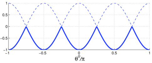
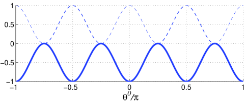
Figure 5: (Color online) Classical $\bar{\cal F}_{\rm cl}^{(1/2)}(\theta^{0})$ (top) and renormalized $\bar{\cal F}^{(1/2)}(\theta^{0})$ (bottom) effective potentials (shown in bold) for the charge mode at density $m=1/2$ in the case of $K\!\gg\!1$, Eqs. (79) and (84) correspondingly

For large but finite $K$, the soliton sizes ${l_{\rm ch}}_{,1/2}$, ${l_{\rm fl}}_{,1/2}$, and the renormalized minigap $\Delta_{\rm ch,1/2}\simeq K\hbar v/{l_{\rm ch}}_{,1/2}$ can be found from the variational estimate of the form (69),

$${K\over{l_{\rm ch}}^{2}_{,1/2}}+{1\over{l_{\rm fl}}^{2}_{,1/2}}+g_{1/2}\left({{l_{\rm fl}}_{,1/2}\over a}\right)^{-1}\left({{l_{\rm ch}}_{,1/2}\over a}\right)^{-\eta},$$ (85)

yielding [$\eta\equiv K^{-1/2}$, $\kappa=(K-1)/K$]

$$\Delta_{\rm ch,1/2}\simeq K^{1-2\eta\over 2-2\eta}\,D\,\left[\kappa|v_{1/2}(2\tilde{A})|\left({\Delta_{0}\over\epsilon_{0}}\right)^{2}\right]^{1\over 1-\eta}.$$ (86)

The value of the gap (86) is strongly enhanced by the bandwidth $D$ [even stronger than for the integer$-m$ case of Sec. VI.1] due to flavor fluctuations. We also note the $m=1/2$ incompressible state is explicitly interaction-induced. Indeed, although the charge excitation gap $\Delta_{\rm ch,1/2}$ is derived in the strongly interacting limit $K\gg 1$, Eq. (86) gives a correct noninteracting limit $\Delta_{\rm ch,1/2}=0$ expected from the single particle Bloch theory. Formally, when $K=1$, both flavor and charge gaps are zero since the last two terms of the potential (77) vanish ($\kappa\to 0$).

The weak coupling estimate (86) is valid when the flavor soliton size (81) is large,

$${l_{\rm fl}}_{,1/2}\gg\lambda_{\rm ext}\,,$$ (87)

according to the condition (58) above. Practically, due to the large bandwidth $D$, Eq. (87) requires rather small bare gap $\Delta_{0}$. For typical parameter values, $\lambda_{\rm ext}\sim 0.1~{}\mu$m and $\Delta_{0}=10$ meV, the soliton scale defined in Eq. (81) is small compared to the potential period $\lambda_{\rm ext}$, ${l_{\rm fl}}_{,1/2}\sim 10\,$nm$\,<\lambda_{\rm ext}$, and the condition (87) does not hold. In this case the excitation gap is given by the strong coupling limit expression (103) (Section VII below).

However, the result (86) is applicable for realistic parameter values, whenever the flavor soliton size ${l_{\rm fl}}_{,1/2}$ becomes large: Either when one takes the tube that is almost metallic, $\Delta_{0}\sim 1$ meV, in which case ${l_{\rm fl}}_{,1/2}\sim 1\,\mu{\rm m}>\lambda_{\rm ext}$, or close to certain potential amplitude values $A^{*}$ that correspond to zeroes of $v_{1/2}(2\tilde{A})$ (Fig. 8).

In the special case when the potential amplitude is such that the coupling $g_{1/2}$ vanishes, $v_{1/2}(2\tilde{A})=0$, the charged excitation is gapless [similar to the integer $m$ case considered above, where the gaps (73) vanish at the zeroes of the Bessel functions], but the flavor sector remains gapped. Its gap $\Delta_{\rm fl}$ can be estimated from the effective O(6)$\simeq$SU(4) Gross-Neveu Lagrangian of the form (75) that is given by the last term of the Lagrangian (77), where now the coupling $g_{\rm GN}\propto u_{1/2}(2\tilde{A}^{*})\neq 0$ (Fig. 8). We stress that the resulting Gross-Neveu coupling is a functional of the applied potential and thus, to an extent, can be controlled externally. Physically, the origin of the flavor gap corresponds to the additional cost of destroying the flavor order in a commensurate state by adding an extra electron of a particular flavor. Naturally, $\Delta_{\rm fl}\sim K^{-1/2}\Delta_{\rm ch}$ is controlled by the strength of the exchange interaction.

VII Strong coupling limit

VII.1 The Lagrangian for the charge sector

Under the condition (61), the Wigner crystal saddle point (60) combined with integrating over the flavor fluctuations yields the following Lagrangian for the charged mode [cf. Eq. (66)]:

$${\cal L}_{\rm charge}[\theta^{0}]={\hbar v\over\pi}\left\{\frac{1}{2v^{2}}(\partial_{t}\theta^{0})^{2}-\frac{K}{2}(\partial_{x}\theta^{0})^{2}\right.$$

$$\left.-gf_{1}\cos(4\theta^{0}+m_{\rm tot}k_{\rm ext}x-8\tilde{A}\sin k_{\rm ext}x)\vphantom{\int}\right\}.$$ (88)

Here the density (1) is related to the chemical potential $\mu$ by Eq. (40), $8\tilde{\mu}\to m_{\rm tot}$, and the coupling constant $g$ is given by its renormalized value (45).

The Lagrangian (88) describes the effective theory of a single mode in the presence of the external potential that is adiabatic on the scale ${l_{\rm fl}}$. This is a result of integrating out the three neutral modes, whose effect has been to produce the Wigner crystal saddle point [Sec. V.1] and to renornalize the coupling $g$. As a result, the number of degrees of freedom in the theory (88) is significantly reduced. This simplification is justified under the following assumptions: (i) separation of charge and flavor energy scales $\Delta_{\rm ch}\gg\Delta_{\rm fl}$ (for that, strong interactions $K\gg 1$ are crucial); (ii) dilute limit $\bar{\rho}{l_{\rm fl}}\ll 1$ that ensures exponentially small flavor-flavor correlations. These conditions imply that the flavor physics is decoupled from the charged one. In other words, the allowed flavor configurations in a train of composite solitons that represent electrons at low density enter with equal weights, which allows us to trace over them, effectively eliminating them from the action. Physically, such a situation corresponds to the limit when the temperature $T\to 0$ and exchange scale $\Delta_{\rm fl}\to 0$ in such a way that $\Delta_{\rm fl}/T\to 0$.CZ ; BalentsFiete

We stress that in the limit (61), the renormalized coupling $g\simeq 1/{l_{\rm fl}}^{2}$ in the Lagrangian (88) does not depend on the density and on the external potential. This is contrary to the weak coupling case of Section VI where the renormalization of nonlinear couplings was sensitive to $m$ and $A$. The reason for this sensitivity in the weak coupling limit is in the flavor soliton size ${l_{\rm fl}}$ (that controls the scale over which the fluctuations are accumulated) extending over a few potential periods. Naturally, in that case the form of $U(x)$ must influence the RG flow.

In the present case, ${l_{\rm fl}}\ll\lambda_{\rm ext}$, and the RG flow produces the effective coupling $g$ [Eq. (45)] on the scale $a<l<{l_{\rm fl}}$ that appears microscopic for the external potential (14). In other words, the adiabatic (on the scales $l\leq{l_{\rm fl}}$) external potential has the effect of the chemical potential that can at best affect the local charge density, but not the RG flow.

VII.2 Refermionization

We now complete our effective single-mode description by refermionizing the theory (88). For that we first present this Lagrangian in the canonical form by rescaling the charge mode:

$$\Theta=2\theta^{0}=\textstyle{\sum}_{\alpha=1}^{4}\Theta_{\alpha}\,.$$ (89)

The field $\Theta$ is the canonical displacement field for the total density,

$$\rho=\frac{1}{\pi}\partial_{x}\Theta\,.$$ (90)

To preserve correct commutation relations, the conjugate momentum $\Pi_{\Theta}$ for the field (89) should be half of that for the field $\theta^{0}$,

$$\Pi_{\Theta}=\textstyle{\frac{1}{2}}\Pi_{\theta^{0}}=\frac{1}{4}\sum_{\alpha=1}^{4}\Pi_{\alpha}\,,$$ (91)

with $\Pi_{\alpha}$ defined in Eq. (27). Changing variables in the Lagrangian (88) according to (89) and (91) we obtain the effective Lagrangian for the mode $\Theta$,

$$\matrix{{\cal L}_{\rm eff}[\Theta]=\displaystyle{\hbar v^{\prime}\over\pi}\left\{\frac{1}{2v^{\prime 2}}\left(\partial_{t}\Theta\right)^{2}-\frac{K^{\prime}}{2}\,\left(\partial_{x}\Theta\right)^{2}\right.\cr\left.-\frac{1}{4}f_{1}g\cos(2\Theta+m_{\rm tot}k_{\rm ext}x-2\tilde{A}^{\prime}\sin k_{\rm ext}x)\vphantom{\displaystyle{\int{1\over v^{2}}}}\right\}}$$ (92)

with the redefined parameters

$$v^{\prime}\equiv 4v\,,\quad K^{\prime}\equiv\textstyle{\frac{1}{16}}K\,,\quad\tilde{A}^{\prime}=4\tilde{A}\equiv\displaystyle{A\over K^{\prime}\hbar k_{\rm ext}v^{\prime}}\,.$$ (93)

The rescaling (93) has the following meaning. The velocity quadrupling simply states that we count incoming fermions regardless of their original flavors. The rescaling of the charge stiffness can be understood by noting that, with the same accuracy that has allowed us to discard the flavor modes [$K\gg 1$, see above],

$$K^{\prime}\approx 1+{(K-1)\over 16}\equiv 1+\nu^{\prime}V(q)\,,\quad\nu^{\prime}={1\over\pi\hbar v^{\prime}}\,,$$ (94)

which is by definition the charge stiffness for the spinless Dirac fermions of velocity $v^{\prime}$ and density of states $\nu^{\prime}$ [cf. Eq. (33)]. Finally, the external fields $U$ and $\mu$ are not rescaled [cf. Eqs. (39) and (37)].

Refermionizing the Lagrangian (92) by introducing the Dirac spinors $\Psi\simeq(2\pi a^{\prime})^{-1/2}e^{i\Theta}$, we formally obtain the effective Hamiltonian

$$\matrix{{\cal H}_{\rm eff}[\Psi]=\displaystyle{\int}\!dx\,\Psi^{+}\left\{-i\hbar v^{\prime}\sigma_{3}\partial_{x}+\Delta^{\prime}\sigma_{1}+U(x)\right.\cr\left.-\mu\right\}\Psi+\displaystyle{\frac{1}{2}}\sum_{k}\rho_{-k}V(k)\rho_{k}}$$ (95)

for the fictitious spinless Dirac fermions. These are the NT electrons averaged (traced) over their SU(4) flavor configurations with equal weights. Naturally, the total fermion number density (6) in the new variables

$$\rho(x)=\Psi^{+}\Psi\,.$$ (96)

The effective gap $\Delta^{\prime}$ in Eq. (95) is chosen in such a way that it corresponds to the renormalized coupling (45) entering the Lagrangian (92),

$${f_{1}\over 4}g\simeq{\Delta^{\prime}\over\hbar v^{\prime}a^{\prime}}\,,\quad a^{\prime}\simeq{l_{\rm fl}}$$ (97)

similarly to the definition (38). In Eq. (97) the new length scale cutoff $a^{\prime}$ is assumed since the present approach is valid only at the length scales $l>{l_{\rm fl}}$ beyond the correlation length of the neutral sector.log Eq. (97) together with Eqs. (45) and (64) estimates

$$\Delta^{\prime}\simeq{\hbar v^{\prime}\over{l_{\rm fl}}}\simeq D^{1/5}\Delta_{0}^{4/5}\,.$$ (98)

To summarize, the NT electron dynamics in the dilute limit (61) is described by the effective Hamiltonian (95) of spinless Dirac electrons. These fictitious fermions of the density (6) carry unit charge, and interact with each other and with external fields in a standard way.

VII.3 Excitation gaps

The (charge) excitation gaps can be now estimated from the effective Lagrangian (92) or from the Hamiltonian (95). Below we assume sufficiently long range interaction

$${l_{\rm ch}}>\lambda_{\rm ext}$$ (99)

in which case the charge excitation is extended over several potential minima, and the single-mode phase soliton approach [Sec. V.3] applies, with the system (92) of the form (54) with $K\to K^{\prime}$, $b\to 2\tilde{A}^{\prime}$, $\beta=2$, and with the period ratio defined in terms of the total density, $m\to m_{\rm tot}$.

The excitation gaps are then obtained in a standard way: According to Sec. V.3, when the total density $m_{\rm tot}$ is integer, one averages the potential term in Eq. (92) over the period obtaining the effective coupling

$$\bar{g}=gJ_{m_{\rm tot}}(2\tilde{A}^{\prime})\,,$$ (100)

then integrates over the fluctuations of the $\Theta$-field

$$\bar{g}(l)=\bar{g}(a^{\prime})\left({l\over a^{\prime}}\right)^{-\eta^{\prime}},\quad\eta^{\prime}=\displaystyle{1\over\sqrt{K^{\prime}}}\simeq 4\eta\ll 1\,,$$ (101)

with $K^{\prime}$ given by Eq. (94) and $\eta$ by Eq. (68), finds the corresponding charge soliton scale self-consistently as

$$\bar{g}({l_{\rm ch}})\simeq\displaystyle{K^{\prime}\over{l_{\rm ch}}^{2}}\,,$$ (102)

and obtains the excitation gap $2\bar{\Delta}_{m}$, where

$$\bar{\Delta}_{m}\simeq\left|J_{m_{\rm tot}}(2\tilde{A}^{\prime})\right|^{\frac{1}{2-\eta^{\prime}}}\bar{\Delta}\,,\quad m_{\rm tot}=4m=\pm 1,\pm 2,...\,.$$ (103)

Here the charge gap

$$\bar{\Delta}\simeq K^{\frac{1-\eta^{\prime}}{2-\eta^{\prime}}}\Delta^{\prime}\,,$$ (104)

with $\Delta^{\prime}$ given by Eq. (98), and $J_{m_{\rm tot}}\equiv J_{4m}$ is the Bessel function that depends on the total density (1).

When the density $m_{\rm tot}=p^{\prime}/q^{\prime}$ is a simple fraction, the charge density in the commensurate configuration is $q^{\prime}\lambda_{\rm ext}-$periodic [as shown in Fig. 1(a) for $m_{\rm tot}=1/2$]. The gaps then follow from the standard phase soliton approachBak [Sec. V.3] which we will not repeat here.

VII.4 Classical limit

The classical limit of the Hamiltonian (95) is obtained by discarding the ${\cal O}(\eta^{\prime})$ quantum fluctuations, and coarse-graining beyond the length scale ${l_{\rm fl}}$, effectively treating electrons as distinguishable point particles [on the scale $l>{l_{\rm fl}}$] that interact with each other via the Coulomb potential (7). The classical energy of this system

$$\matrix{\displaystyle{E}_{\rm cl}=\sum\left[\Delta^{\prime}+U(x_{i})\right]\ +\ \sum\left[\Delta^{\prime}-U(y_{j})\right]\cr\displaystyle{+}\sum_{i>i^{\prime}}V(x_{i}-x_{i^{\prime}})+\sum_{j>j^{\prime}}V(y_{j}-y_{j^{\prime}})-\sum_{i,j}V(x_{i}-y_{j}).\quad}$$ (105)

Here the indices $i,i^{\prime}$ and $j,j^{\prime}$ run over electrons (with positions $x$) and holes ($y$), correspondingly, in the minima and in the maxima of the potential (14). The incompressible states are parametrized by the pairs $(n_{e},n_{h})$ of rational numbers of electrons and holes per period $\lambda_{\rm ext}$ according to Eq. (2) [cf. Section I and Fig. 1].

The connection between the classical limit (105) of the effective Hamiltonian (95), and the original charge mode Lagrangian (92) follows from representing the coordinates of electrons by

$$x_{j}=x_{j}^{(0)}+\phi_{j}\,,$$ (106)

where $\phi_{j}$ are the displacements from the ideal positions

$$x_{j}^{(0)}={j\lambda_{\rm ext}\over m_{\rm tot}}\,,\quad j=1,2,...$$ (107)

in the Wigner crystal in the absence of the external potential. [For simplicity, we are not considering the holes in the maxima of $U(x)$, which can be treated analogously.] In the continual limit $\phi_{j}\equiv\phi(x_{j})\approx\phi(x)$ the charge density is

$$\rho(x)\approx{m_{\rm tot}\partial_{x}\phi\over\lambda_{\rm ext}}\,,$$ (108)

describing the change of $\phi$ by $\lambda_{\rm ext}/m_{\rm tot}$ when one extra particle is added. The third sum in Eq. (105) gives the interaction energy between the electrons. Substituting the coordinates (106) into this sum and expanding it up to the second order in $\phi_{i}-\phi_{j}\approx\left(x_{i}^{(0)}-x_{j}^{(0)}\right)\partial_{x}\phi$, we obtain the gradient term for the displacement mode energy,

$$\frac{1}{2}\int\!dx\,\left(2e^{2}\ln\tilde{N}\right)\rho^{2}(x)\equiv{\hbar v^{\prime}\over\pi}\int\!dx\,{\tilde{K}^{\prime}(\partial_{x}\Theta)^{2}\over 2}\,,$$ (109)

where

$$\Theta={\pi m_{\rm tot}\over\lambda_{\rm ext}}\phi(x)$$ (110)

is the net charge mode (89) defined in accord with the expression (90) for the total charge density, and the charge stiffness

$$\tilde{K}^{\prime}={1\over\pi\hbar v^{\prime}}\cdot 2e^{2}\ln\tilde{N}\simeq K^{\prime}-1\approx K^{\prime}\,.$$ (111)

Here the stiffness $K^{\prime}$ is defined in Eq. (94), and the argument $\tilde{N}$ of the Coulomb logarithm is found self-consistently as a number of electrons whose positions are altered in a charged phase-soliton excitation. The expression (109) is the classical limit of the second term of the Lagrangian (92) with a meaning of the Coulomb interaction between the quasi-classical electrons. The nonlinear term of the Lagrangian (92) gives the bare energy cost $\Delta^{\prime}\cos\left(m_{\rm tot}k_{\rm ext}\delta\phi\right)=\Delta^{\prime}$ of adding a particle above the gap (modulo interactions), with $\delta\phi=\lambda_{\rm ext}/m_{\rm tot}$ according to Eq. (108). This term corresponds to the constant term in the classical energy (105), $\sum_{x_{i}}\Delta^{\prime}$. The interaction with the potential, $\sum_{x_{i}}U(x_{i})$, can be written in the usual form (13) and added to the argument of the cosine via the gauge transformation (32).

VII.5 Discussion

The main result of this Section is the single-mode effective Hamiltonian (95) that has allowed us to map the problem of the interacting fermions with the four flavors onto that of a single flavor and to utilize the standard phase soliton approach for the single mode.

The physical meaning of the present treatment is as follows. In the noninteracting case, fermions of the same flavor avoid each other due to the Pauli principle. The ground state wave function is then given by a product of the four Slater determinants, one for each flavor. However, when the repulsion between the fermions is strong, fermions of all the flavors avoid each other in a similar way, and the ground state wave function is a Slater determinant of a four-fold size.Ogata This is manifest in the $m_{\rm tot}=4m-$dependence of the excitation gaps (103).

The original SU(4) flavor symmetry of the problem becomes manifest on the level of renormalization, namely in the particular scaling law of $4/5$ of the renormalized gap (98) produced by the renormalization group flow of the flavor sector on the length scales $a<l<{l_{\rm fl}}$.

Let us compare the scaling laws in Eqs. (103) and (104) with those obtained in the weak-coupling limit. In the classical limit the charge excitation gap (104) for the stand-alone nanotube has the same form as that obtained in Sec. V.5 above, Eq. (67):

$$\bar{\Delta}=\Delta\quad{\rm when}\quad K\to\infty\,.$$ (112)

However, one notes that at finite $K$, the power law exponents in the expressions (104) and (103) are different from those in Eqs. (71) and (73). This is not surprising since the theory (88) is different from the original model (35). Whereas in the latter the exchange is important, in the former the flavor sector is traced over under the assumptions specified above in Sec. VII.1; different theories indeed yield different scaling laws. A similar subtlety in taking the order of limits of vanishing temperature and exchange was observed in the recent calculation of correlation functions CZ for spin$-1/2$ fermions, and was qualitatively explained in Ref. BalentsFiete, . In the present case, the same phenomenon is manifest in the scaling behavior of the excitation energy.

We underline that the external potential (14), by adding an extra length scale $\lambda_{\rm ext}$, naturally distinguishes the regimes ${l_{\rm fl}}>\lambda_{\rm ext}$ and ${l_{\rm fl}}<\lambda_{\rm ext}$ in which the flavor physics is important and unimportant, correspondingly. Accordingly, the dependence on the parameters of the potential in these two regimes is also qualitatively different, as one may see by comparing e.g. Eqs. (73) and (103) even in the limit $K\to\infty$.

VIII Phase diagram

Below we draw the phase diagram for the classical system (105) in the $A,\mu$ plane, Fig. 6, where $A$ is the potential amplitude in Eq. (14). Here we assume that the screening length is larger than the length $L$ of the system,

$$l_{s}\sim{l_{\rm ch}}>L\equiv N\lambda_{\rm ext}$$ (113)

(effectively meaning that ${l_{\rm ch}}=\infty$), thus the charged phase-soliton optimization of an excitation (described in Sec. V.3) does not take place. In the limit (113), by raising the chemical potential one adds electrons (holes) to the sequence of “quantum dots” ( “anti-dots”) evenly over all the system, changing the commensurate density $m_{\rm tot}$ from one rational number to another. Each region in Fig. 6 corresponds to a particular commensurate phase $(n_{e},n_{h})$ (as described in Section I), with density (2). Borders separating regions with integer $(n_{e},n_{h})$ are comprised of fractional-density states, such as the domain $(1/2,0)$ between $(0,0)$ and $(1,0)$ [charge state sketched in Fig. 1(a)]. At zero temperature, all the commensurate charge states (rational $m_{\rm tot}=p^{\prime}/q^{\prime}$) are incompressible, with a spectrum being a devil’s staircase. At finite temperature gaps for sufficiently large denominator $q^{\prime}$ will be washed out. The underlying Dirac symmetry makes the phase diagram symmetric with respect to $\mu\leftrightarrow-\mu,\ n_{e}\leftrightarrow n_{h}$, so that only the $\mu>0$ part is shown.

The phase diagram is obtained by minimizing the energy functional

$$E_{n_{e},n_{h}}(A)-\mu(n_{e}-n_{h})\,,\quad E_{n_{e},n_{h}}=\textstyle{\frac{1}{N}}E_{\rm cl}(x_{i},y_{j})$$ (114)

[$E_{\rm cl}$ given by Eq. (105)], with respect to positions $x_{i}$ and $y_{i}$ of electrons and holes in the following way. For large size $N$, we neglect finite size effects and utilize translational invariance. In this case, in a commensurate state, the optimal positions of electrons and holes relative to each potential minimum (maximum) are the same for each period. The result is the family of system’s charging energy values $E_{n_{e},n_{h}}(A)$ per period $\lambda_{\rm ext}$, such as

$$E_{10} = \Delta^{\prime}-A+{e^{2}\over\lambda_{\rm ext}}\sum_{n=1}^{N/2}{1\over n}\,,$$ (115)

$$E_{11} = 2E_{10}-{2e^{2}\over\lambda_{\rm ext}}\sum_{n=1}^{N/2}{1\over n-\frac{1}{2}}\,,$$ (116)

$$E_{20}=\mathop{{\rm min}}_{\delta x}\left\{\vphantom{{{{{{X^{X}}^{X}}^{X}}^{X}}^{X}}^{X}}2\Delta^{\prime}-2A\cos k_{\rm ext}\delta x+{e^{2}\over 2\delta x}\right.$$

$$\left.+{e^{2}\over\lambda_{\rm ext}}\sum_{n=1}^{N/2}\left({2\over n}+{1\over n+{2\delta x/\lambda_{\rm ext}}}+{1\over n-{2\delta x/\lambda_{\rm ext}}}\right)\right\}\quad$$ (117)

[here $\pm\delta x$ is the electron coordinate relative to the minimum of $U(x)$], and so forth. While minimizing the energy $E_{n_{e},n_{h}}$ with respect to the positions of electrons and holes within each potential period, unphysical configurations of electrons on top of the holes are excluded by demanding that their minimum separation be $e^{2}/\Delta^{\prime}$. The latter condition takes into account exciton binding energy in the Dirac system.

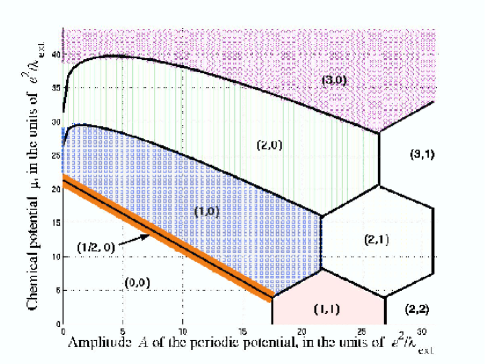
Figure 6: (Color online) Phase diagram for the nanotube, $\Delta^{\prime}=6\pi e^{2}/\lambda_{\rm ext}$, $\ln(L/\lambda_{\rm ext})=2.5$, $e^{2}/\lambda_{\rm ext}=1.44$ meV for $\lambda_{\rm ext}=1\mu$m. Shaded regions are the result of the numerical minimization of Eq. (114) (see text), black lines are approximations obtained from Eq. (118) with $V_{n}$ given by Eq. (123).

The functional $E_{n_{e},n_{h}}(A)$ can be further approximated by minimizing the interaction energy between the charges only in the same potential minimum (or maximum), treating the rest of the system in a mean-field way:

$$E_{n_{e},n_{h}}\approx(n_{e}+n_{h})(\Delta^{\prime}-A)+{(n_{e}-n_{h})^{2}e^{2}\over 2C_{0}}+V_{n_{e}}+V_{n_{h}}\,.$$ (118)

The first term in (118) is the energy of $n_{e}$ electrons placed into each minimum and $n_{h}$ holes into each maximum of $U(x)$. It corresponds to the first two terms of (105). The second term in (118) is the interaction energy of the electrons and holes located in the extrema of $U(x)$. Here

$$C_{0}\simeq{\lambda_{\rm ext}\over 2\ln(L/\lambda_{\rm ext})}$$ (119)

is the NT capacitance per period $\lambda_{\rm ext}$. Finally, $V_{n}$ in (118) is the interaction energy of $n$ electrons (or $n$ holes) minimized with respect to their positions inside the corresponding potential well of the periodic potential (14). The Dirac symmetry yields $E_{n_{e},n_{h}}=E_{n_{h},n_{e}}$. Minimization of Eq. (114) using the approximation (118) yields the phase diagram sketched in Fig. 7. In the limit (113), excitation gaps corresponding to the incompressible states with the total density $n=n_{e}-n_{h}=(n_{e}+1)-(n_{h}+1)=...=(n_{e}+s)-(n_{h}+s)$ oscillate but do not vanish. Their minimum value

$$\delta\mu_{n_{e},n_{h}}^{\rm min}={e^{2}\over C_{0}}$$ (120)

is determined by the NT charging energy. The regions $(n_{e},n_{h})$ and $(n_{e}+1,n_{h}+1)$ of the phase diagram are separated by the vertical lines of fixed $A$, with its value implicitly determined from

$$A=\Delta^{\prime}+\textstyle{\frac{1}{2}}\left\{V_{n_{e}+1}(A)-V_{n_{e}}(A)+V_{n_{h}+1}(A)-V_{n_{h}}(A)\right\}.$$ (121)

Away from the values (121) the gap increases $\propto A$.

The mean field approximation (118) produces fairly accurate borders between the domains of the phase diagram in Fig. 6. Below we consider the quantum-dot addition energies $V_{n_{e}}$ for the small and large $n_{e}$.

VIII.1 Small density $n_{e},n_{h}\sim 1$

First consider the situation when the Coulomb interaction over a period is small, ${e^{2}/\lambda_{\rm ext}}\ll A$, such that $n_{e}$ electrons are grouped close to the minima of the potential that can be approximated by a piecewise-quadratic polynomial:

$$U(x)\approx-A+{\rm min}_{n\leq N}\frac{Ak_{\rm ext}^{2}}{2}\left(x-(n+\textstyle{\frac{1}{2}})\lambda_{\rm ext}\right)^{2}.$$ (122)

Minimizing the Coulomb energy of $n_{e}$ charges in a single minimum of the potential (122), one obtains the values

$$\matrix{V_{0}=V_{1}=0\,,\cr V_{2}=3\,(\pi/2)^{2/3}\left({e^{2}\over\lambda_{\rm ext}}\right)^{2/3}A^{1/3}\,,\cr V_{3}=5^{2/3}V_{2}(A)\,,\,...\,.}$$ (123)

The power law correction $\sim A^{1/3}$ due to the above expressions is observed in Fig. 6 for $A\sim\Delta^{\prime}$ as a deviation from the straight lines that separate different regions of the phase diagram.

When, on the other hand, the periodic potential is a small perturbation that shifts electrons from their equidistant position in a Wigner crystal ($A\ll e^{2}/\lambda_{\rm ext}$), the perturbation theory in $A$ yields analytic behavior of the gap widths on $A$.

Figure 7: Phase diagram in the $(A,\mu)$ plane according to the model (118). The minimum width of the gap for the incompressible state with any integer density $n_{e}-n_{h}$ is given by the NT charging energy (120). In the limit $n_{e},n_{h}\gg 1$ all the regions of the phase diagram are identical, with their period in $A$ given by Eq. (128).

VIII.2 Large density $n_{e},n_{h}\gg 1$

At large $n_{e},n_{h}\gg 1$ the model (118) can be simplified by using the continuous Thomas-Fermi description for the density of the classical electrons (holes) inside each potential minimum (maximum). To find $V_{n_{e}}$, we approximate the local charge density as

$$\rho(x)\approx\rho_{\rm TF}=-{\pi n_{e}\over\lambda_{\rm ext}}\cos k_{\rm ext}x\,,$$ (124)

that mimics the external potential profile (14). The density (124) is normalized to $n_{e}=\int_{\lambda_{\rm ext}/4}^{3\lambda_{\rm ext}/4}\rho_{\rm TF}(x)dx$. The interaction energy $V_{n_{e}}$ or $V_{n_{h}}$ inside each “quantum dot” can be estimated as

$$V_{n_{e}}\simeq{e^{2}\over 2}\int_{\lambda_{\rm ext}/4}^{3\lambda_{\rm ext}/4}\!dxdx^{\prime}\,{\rho_{\rm TF}(x)\rho_{\rm TF}(x^{\prime})\over|x-x^{\prime}|}\equiv{n_{e}^{2}e^{2}\over 2C_{1}}\,,$$ (125)

where the “dot capacitance”

$$C_{1}\simeq{\lambda_{\rm ext}\over 2\pi\ln{\lambda_{\rm ext}\over a^{\prime}}}$$ (126)

is independent of the potential amplitude $A$. The log singularity in the integral in Eq. (125) is cut off on the scale $a^{\prime}\sim{l_{\rm fl}}$ of the order of the flavor soliton size, below which the quasiclassical description breaks down (see Section VII). The $A$–dependence of $C_{1}$ would appear as a correction to $V_{n_{e}}$ with $A$–dependent integration limits in Eq. (125). The case $V_{n_{h}}$ of the holes in the potential maxima (“anti-dots”) is analogous. Eq. (121) then yields the potential amplitude values that separate the configurations $(n_{e},n_{h})$ and $(n_{e}+1,n_{h}+1)$:

$$A_{(n_{e},n_{h})\to(n_{e}+1,n_{h}+1)}=\Delta^{\prime}+{e^{2}\over 2C_{1}}(n_{e}+n_{h}+1)\,.$$ (127)

In this limit all the honeycomb regions in Fig. 7 are identical with their size in $A$ being

$$\delta A_{n_{e},n_{h}}={e^{2}\over C_{1}}\,.$$ (128)

Qualitatively, the regular honeycomb structure of Fig. 7 appears already for moderate amplitudes $A$ (Fig. 6). The borders between the regions of the diagram in the limit $A>e^{2}/\lambda_{\rm ext},\Delta^{\prime}$, are approximately linear, dominated by the linear dependence of $E_{n_{e},n_{h}}$ on $A$ that stems from the first term of Eq. (118).

VIII.3 Crossover with the case ${l_{\rm ch}}<L$

We will now show that the asymptotic values of the positions (127) of the gap minima derived above for large $n_{e}$ and $n_{h}$ coincide with those obtained in Section VII utilizing the phase soliton method in an infinite system. For this crossover we assume ${l_{\rm ch}}\sim l_{s}\sim\lambda_{\rm ext}$.

Consider the positions of the minima for excitation gaps (103) (as a function of the potential amplitude)

$$\tilde{A}^{\prime}=4\tilde{A}={4A\over K\epsilon_{0}}\approx{\pi\over 2}\cdot{A\over e^{2}/C_{1}}\,,$$ (129)

where we took the value of the charge stiffness (33) at the momentum scale $\lambda_{\rm ext}^{-1}$ and substituted $K\to K-1$ at $K\gg 1$. Utilizing the asymptotic behavior of the $n-$th zero of the Bessel function $J_{m_{\rm tot}}$,

$$2\tilde{A^{\prime}}_{m_{\rm tot}}^{(n)}\simeq{\rm const}\,+{\pi m_{\rm tot}\over 2}+\pi n\,,\quad n={\rm min\,}\{n_{e},n_{h}\}\,,$$ (130)

we indeed obtain the values $A\simeq(n_{e}+n_{h})e^{2}/2C_{1}$ corresponding to gap minima in accord with Eq. (127).

IX Experimental means to probe incompressible states

IX.1 Conductance measurements

Excitation gaps corresponding to the incompressible states can be detected in transport measurements. When, by means of varying the gate voltage, the Fermi level is tuned to be in the gap, the zero-bias conductance $\sigma$ across the nanotube vanishes. At finite temperature $T$, $\sigma$ will have the activated form

$$\sigma\sim e^{-T_{\rm act}/T}\,,$$ (131)

with the activation energy $T_{\rm act}=\Delta_{m}$ equal to half of the excitation gap corresponding to a particular incompressible state. Physically, Eq. (131) corresponds to the transport by means of thermally-excited charge solitons that can carry electric current through the nanotube. (A similar situation has been recently considered in the context of transport in granular arrays.AGK ) The values and positions of the gaps can be also revealed by measuring the differential conductance at finite bias with varying gate voltage. In this case, peaks in the differential conductance as a function of the applied bias will mark the positions of the excitation gaps.

IX.2 Adiabatic charge pumping

A more challenging possibility is to realize the Thouless pumpThouless in a nanotube. Such a setup requires an adiabatically moving periodic potential that could be created e.g. by coupling to a surface acoustic wave (SAW),Talyanskii'01 or by sequentially modulated gate voltages on the array of underlying gates. When the chemical potential is inside the $m$-th minigap $\Delta_{m}$, the adiabatically moving periodic potential with frequency $f$ induces quantized current Talyanskii'01

$$j=m_{\rm tot}ef\,,\quad m_{\rm tot}=4m\,.$$ (132)

In such a setting, novel fractional-$m$ incompressible states considered in this work will manifest themselves in the adiabatic current (132) quantized in the corresponding fractions of $4ef$.NT-devil This result can be understood by invoking the topological invariant property of the Thouless current.Thouless ; niu-thouless The expression (132) is trivial in a semiclassical limit, with a meaning of transporting on average $m_{\rm tot}$ electrons per cycle in a conveyer-belt fashion. By staying inside the gap and adiabatically changing the parameters of the system, the current (132) remains invariant and hence it is valid in the fully quantum-mechanical case.

Operation of the charge pump requires adiabaticity

$$k_{B}T,\ hf\ll\Delta_{m}\,.$$ (133)

Since the energy scale for the minigaps is set either by the gap $2\Delta_{0}$ at half-filling, or by the strength of the Coulomb interactions between electrons separated by $\sim\lambda_{\rm ext}$, the typical minigap values $\Delta_{m}$ are in the meV range, and the adiabaticity condition (133) is realistic. The feasibility of the Thouless pump in the NT-SAW setup is further corroborated by recent pumping experiments involving SAWs. In particular, in the pumping of electrons between the two 2D electron gases through a pinched point contact Shilton the achieved quality of current quantization is close to metrological.niu'90 ; current-standard Recently the SAW-assisted pumping has been demonstrated through the laterally defined quantum dot,screw as well as through the semiconducting nanotube whose working length $L$ matched the SAW period, $L=\lambda_{\rm ext}$.Ebbecke'04 ; Leek

We contrast the non-dissipative current (132) on the plateau with the dissipative non-quantized current away from commensuration considered in Ref. Niu, for arbitrary quantum wire. Such a non-quantized current is pumped when no gap opens (for incommensurate densities or for commensurate densities with the interaction below criticality) and is characterized by the interaction-dependent critical exponents.Niu

A practical realization of the proposed pumping setup can become a first implementation of the Thouless transport. Besides being instrumental in studying electron interactions in a nanotube (by detecting and measuring fractional$-m$ minigaps that arise solely due to interactions), it could realize the “conveyer belt” for electrons with a possibility of pumping current quantized in fractions of the unit charge per cycle. In other words, such a setup would make the first example of the charge pump operating at the fraction of the base frequency. This setup could allow one to study in detail the electron correlations and interactions in nanotubes, with a variety of controllable parameters at hand, such as the shape and frequency of the external potential, nanotube gap $\Delta_{0}$ (that can be modified externally), and the gate voltage. By exploring the phase diagram one can study effects of Wigner crystallization, quantum commensurate-incommensurate transitions, and the Tomonaga-Luttinger correlations.

Finally, we note that the described setup can be utilized to adiabatically transport low-energy strongly correlated SU(4) flavor states [e.g. those for $m=1/2$ obeying the effective Gross-Neveu Lagrangian of the form (75) described in Sec. VI] over a macroscopic distance, since the coupling to the adiabatically moving external potential is SU(4) invariant and thus it does not destroy spin or flavor correlations. This may become useful in the context of solid state implementations of quantum information processing. Furthermore, this setup can provide a possibility of realizing a quantized spin-polarized pump by subjecting the system to magnetic field tuned in such a way that only one spin population of electrons is commensurate with the potential and participates in current quantization.

X Conclusions

In the present work we have shown that coupling of the interacting electrons in a nanotube to an external periodic potential is a rich setup to study one-dimensional electronic correlations, including the crossover between the Luttinger liquid and the Wigner crystal. We demonstrated that the external potential locks the system into incompressible states. The corresponding excitation gaps (estimated to be in meV range) are found by adequately treating the curvature of the electronic dispersion in the bosonized language, and by further generalizing the phase soliton method onto the case of multiple modes.

In the regime when the gaps open due to the Bragg diffraction in a multi-flavor Luttinger liquid, we identified and investigated the novel incompressible fractional-density state with $m=1/2$ electrons of each flavor per period of the potential. The phase soliton action derived for this case describes the charge excitation, and the SU(4)-flavor excitations governed by the O(6) Gross-Neveu model.

In the opposite limit of the pinned Wigner crystal we derived the effective single-mode Hamiltonian and found that the phase diagram in the classical limit has a stucture of the devil’s staircase.

The interaction-induced incompressible states can be detected in the Thouless pump setup that can allow one to study electron correlations and the transition to the Wigner crystal, as well as to realize the quantized charge pump that operates at a fraction of the base frequency by virtue of electron-electron interactions.

Appendix A Conditions for the tight-binding limit

Below we derive the condition (26) for the tight binding limit (25) in the single particle picture. We consider the two cases depending on the relation between the potential amplitude $A$ and the Dirac mass term $\Delta_{0}$.

The case $A\ll\Delta_{0}$ corresponds to the “nonrelativistic limit” of the Dirac equation, where all the relevant energies are much smaller than the gap $\Delta_{0}$. We define the “Dirac” electron mass $M$ via $\Delta_{0}=Mv^{2}$, and turn to the effective Schrödinger description with the Hamiltonian

$${\cal H}_{\rm Sch}=-{\hbar^{2}\over 2M}\,\partial_{x}^{2}+U(x)\,,$$ (134)

in full analogy with the non-relativistic limit in QED. The tunneling amplitude between the adjacent minima of $U(x)$ is proportional to $e^{-S|_{A<\Delta_{0}}/\hbar}$, where the classical action under the barrier

$${S|_{A<\Delta_{0}}}={4\hbar\sqrt{A\Delta_{0}}\over\epsilon_{0}}\,.$$ (135)

Therefore both the minibands and tunneling are suppressed in the limit $A\ll\Delta_{0}$ if

$$\left({\Delta_{0}\over\epsilon_{0}}\right)^{-1}<{A\over\epsilon_{0}}\ll{\Delta_{0}\over\epsilon_{0}}\,.$$ (136)

The inherently Dirac regime occurs when $A>\Delta_{0}$. In this case electron can tunnel between the minima of the potential (14) sequentially through the hole part of the spectrum. The corresponding tunneling amplitude $\sim e^{-2S|_{A>\Delta_{0}}/\hbar}$, where the classical action for the particle with energy $E$ under barrier between the electron and hole parts is

$$S|_{A>\Delta_{0}}=\frac{1}{v}\int\!dx\,\sqrt{|[E-U(x)]^{2}-\Delta_{0}^{2}|}\,.$$ (137)

Tunneling from the minimum of $U(x)$ at $E=\Delta_{0}-A$ to the hole part of the spectrum yields ($\delta\equiv{\Delta_{0}/A}$)

$$S|_{E=\Delta_{0}-A}={2\hbar A\over\epsilon_{0}}\;\left\{\sqrt{\delta}-\left(1-\delta\right)\ln\frac{1+\sqrt{\delta}}{\sqrt{1-\delta}}\right\}$$

$$={4\hbar\Delta_{0}^{3/2}\over\epsilon_{0}A^{1/2}}\;\left({1\over 1\cdot 3}+{\delta\over 3\cdot 5}+{\delta^{2}\over 5\cdot 7}+\;...\right).$$ (138)

Tunneling from the energy level $|E|\ll A-\Delta_{0}$ far from the potential bottom yields the action $S|_{|E|\ll A-\Delta_{0}}\simeq\pi\Delta_{0}^{2}/\hbar v{\cal E}$, where ${\cal E}=|\partial_{x}U(x)|\simeq k_{\rm ext}A$. The requirement $S|_{E=\Delta_{0}-A}>\hbar$ or $S|_{|E|\ll A-\Delta_{0}}>\hbar$ yields that the single particle bandwidth in the Dirac regime is exponentially suppressed if

$${\Delta_{0}\over\epsilon_{0}}<{A\over\epsilon_{0}}<\left({\Delta_{0}\over\epsilon_{0}}\right)^{c},$$ (139)

where, correspondingly, the exponent $c=3$ for tunneling from the potential minimum and $c=2$ for tunneling from energy level far from the potential bottom.

Summarizing, Eqs. (136) and (139) yield the condition (26) for the tight-binding limit (25).

Appendix B $m=\frac{1}{2}$ phase soliton action

Below we consider the weak coupling limit for the fractional density $m=\frac{1}{2}$, characterized by the chemical potential $\tilde{\mu}=\frac{1}{4}$ in accord with Eq. (40).

Our course of action has been outlined in Section V above. Technically, it will be more convenient to first work in the basis of the original fields $\Theta_{\alpha}$ and later utilize the transformation (29) to obtain the Lagrangian ${\cal L}_{1/2}[{\bar{\theta}^{0},\bar{\theta}^{a}}]$ in the charge-flavor basis. Since the average of the potential energy (37) over the two successive potential periods is zero, we decompose the fields $\Theta_{\alpha}(x)$ in a series in the coupling $g_{0}$ keeping the zeroth and the first orders

$$\Theta_{\alpha}=\bar{\Theta}_{\alpha}+\Theta^{(1)}_{\alpha}\ ,\quad\Theta^{(1)}_{\alpha}={\mathcal{O}}(g_{0})\,.$$ (140)

Figure 8: (Color online) The functions $v_{1/2}$ and $u_{1/2}$ defined in Eqs. (149) and (150). We find that $v_{1/2}(z)<u_{1/2}(z)$ holds for all $z$. Zeroes of $v_{1/2}$: $z=0,\ \pm 2.33,\ \pm 3.80,\ \pm 5.47,...$ .

Consider the Hamiltonian

$${\cal H}^{(1/2)}[\Theta_{\alpha}]={\hbar v\over\pi}\left\{\displaystyle{{1\over 2}}\,\sum(\partial_{x}\Theta_{\alpha})^{2}+\displaystyle{{K-1\over 8}}\,\left(\sum\partial_{x}\Theta_{\alpha}\right)^{2}\right.$$

$$\left.+\displaystyle{\frac{1}{4}}g_{0}\,\sum\cos(2\Theta_{\alpha}+\textstyle{\frac{1}{2}}k_{\rm ext}x-2\tilde{A}\sin k_{\rm ext}x)\right\}.\quad$$ (141)

The Euler-Lagrange equations $\delta{\cal H}^{(1/2)}/\delta\Theta_{\alpha}=0$ are

$$\Theta_{\alpha\ xx}^{(1)}+{K-1\over 4}S^{(1)}_{xx}=-{g_{0}\over 2}\sin(2\bar{\Theta}_{\alpha}+\textstyle{\frac{1}{2}}k_{\rm ext}x-2\tilde{A}\sin k_{\rm ext}x),$$ (142)

where $S=\sum\Theta_{\alpha}$, and $S_{x}\equiv\partial_{x}S$, etc. Integrating Eq. (142) we obtain

$$\Theta_{\alpha\ x}^{(1)} = {1-K\over 4}S^{(1)}_{x}+{g_{0}\over k_{\rm ext}}\,\tilde{\Theta}_{\alpha}\,,$$ (143)

$$\quad S^{(1)}_{x} = {g_{0}\over Kk_{\rm ext}}\,\sum\tilde{\Theta}_{\alpha}\,,$$ (144)

$$\tilde{\Theta}_{\alpha} = \sum_{m}{J_{m}(2\tilde{A})\over 1-2m}\cos\left(2\bar{\Theta}_{\alpha}+(\textstyle{\frac{1}{2}}-m)k_{\rm ext}x\right).\quad$$ (145)

Substituting Eqs. (143) and (145) into the Hamiltonian (141), after somewhat lengthy but straightforward algebra the slow mode potential follows:

$$V_{1/2} = {\hbar vg_{0}^{\prime}\over 16\pi}\left\{\vphantom{\sum_{\alpha\neq\alpha^{\prime}}}(4-\kappa)v_{1/2}\sum_{\alpha}\cos 4\bar{\Theta}_{\alpha}\right.$$ (146)

$$+ \kappa u_{1/2}\sum_{\alpha\neq\alpha^{\prime}}\cos(2\bar{\Theta}_{\alpha}-2\bar{\Theta}_{\alpha^{\prime}})$$

$$- \left.\kappa v_{1/2}\sum_{\alpha\neq\alpha^{\prime}}\cos(2\bar{\Theta}_{\alpha}+2\bar{\Theta}_{\alpha^{\prime}})\right\}.$$

Here

$$g_{0}^{\prime} = \left({g_{0}\over k_{\rm ext}}\right)^{2}=\left({\Delta_{0}\over\epsilon_{0}a}\right)^{2}\,,$$ (147)

$$\kappa = {K-1\over K}\,,$$ (148)

and the couplings $v_{1/2}$ and $u_{1/2}$ are defined as

$$v_{1/2}(z)=\sum_{m=-\infty}^{\infty}{J_{m}(z)J_{1-m}(z)\over(2m-1)^{2}}\,,$$ (149)

$$u_{1/2}(z)=\sum_{m=-\infty}^{\infty}\left({J_{m}(z)\over 1-2m}\right)^{2}$$ (150)

with $z$ being a shorthand for $2\tilde{A}$. The functions $v_{1/2}(z)$ and $u_{1/2}(z)$ are plotted in Fig. 8.

In the commensurate state the minimum value

$${\rm min\ }V_{1/2}[\bar{\Theta}_{\alpha}]=-{\hbar vg_{0}^{\prime}\over 4\pi}\left\{4|v_{1/2}(2\tilde{A})|+\kappa u_{1/2}(2\tilde{A})\right\}$$ (151)

of the potential (146) corresponds to $\{\bar{\Theta}_{\alpha}\}$ being a permutation of a set $\{\phi_{1}\ \phi_{1}\ \phi_{2}\ \phi_{2}\}$, with $\phi_{1,2}=\pm\pi/4$ for $v_{1/2}(2\tilde{A})>0$ and $\phi_{1}=0,\ \phi_{2}=\pi/2$ for $v_{1/2}(2\tilde{A})<0$.

We now discuss the obtained commensurate classical state. The ground state degeneracy in the noninteracting case ($\kappa=0$) is equal to $2^{4}$. This follows from the potential (146) in which only the first term is nonzero. In the presence of interactions ($\kappa>0$), the other terms in (146) reduce this degeneracy from 16 to six. This result could have been foreseen without any calculation since the remaining degeneracy is a number of configurations in which any two different fields, $\Theta_{\alpha}$ and $\Theta_{\alpha^{\prime}}$ with $\alpha\neq\alpha^{\prime}$, are placed in the same minimum of the external potential. In other words, in the bosonized treatment the effect of fermionic exchange manifests itself in a stronger repulsion between the solitons of the same flavor. This is in agreement with the numerical minimization performed in Sec. V.2, Fig. 4. The symmetry of the obtained classical ground state is schematically illustrated in Fig. 1(e).

The change of variables (29) in the potential (146) yields Eq. (77).

References

- (1) S. Iijima, Nature 354, 56-58 (1991).
- (2) R. Saito, G. Dresselhaus and M. S. Dresselhaus, Physical Properties of Carbon Nanotubes, Imperial College Press, London, 1998.
- (3) M.S. Dresselhaus, G. Dresselhaus, Ph. Avouris, Carbon Nanotubes: Synthesis, Structure, Properties and Applications, Springer Verlag, New York, 2001.
- (4) P.L. McEuen, Nature 393, 15 (1998).
- (5) C. Dekker, Physics Today, May 1999, p. 22.
- (6) Y.A. Krotov, D.-H. Lee, S.G. Louie, Phys. Rev. Lett. 78, 4245 (1997).
- (7) R. Egger, A. O. Gogolin, Phys. Rev. Lett. 79, 5082 (1997).
- (8) C. Kane, L. Balents, M. P. A. Fisher, Phys. Rev. Lett. 79, 5086 (1997).
- (9) H. Yoshioka and A.A. Odintsov, Phys. Rev. Lett. 82, 374 (1999).
- (10) L.S. Levitov and A.M. Tsvelik, Phys. Rev. Lett. 90, 016401 (2003).
- (11) M. Stone (Ed.), Bosonization, World Scientific, Singapore (1994)
- (12) M. Bockrath, D. H. Cobden, P. L. McEuen, N. G. Chopra, A. Zettl, A. Thess, R. E. Smalley, Science 275, 1922 (1997).
- (13) S. Tans, M.H. Devoret, R. Groeneveld and C. Dekker, Nature 394 761 (1998).
- (14) M. Bockrath, D. H. Cobden, Jia Lu, A. G. Rinzler, R. E. Smalley, L. Balents, P. L. McEuen, Nature 397, 598 (1999).
- (15) Z. Yao, H. W. Ch. Postma, L. Balents, C. Dekker, Nature 402, 273 (1999).
- (16) J. Nygard, D.H. Cobden, M. Bockrath, P.L. McEuen, P.E. Lindelof, Applied Physics A 69, 297 (1999).
- (17) H. Ishii, H. Kataura, H. Shiozawa, H. Yoshioka, H. Otsubo, Y. Takayama, T. Miyahara, S. Suzuki, Y. Achiba, M. Nakatake, T. Narimura, M. Higashiguchi, K. Shimada, H. Namatame and M. Taniguchi, Nature (London) 426, 540 (2003).
- (18) P. Jarillo-Herrero, J. Kong, H.S.J. van der Zant, C. Dekker, L.P. Kouwenhoven, and S. De Franceschi, Nature (London) 434, 484 (2005).
- (19) M.-S. Choi, R. Lopez, and R. Aguado, Phys. Rev. Lett. 95, 067204 (2005).
- (20) V.I. Talyanskii, D.S. Novikov, B.D. Simons, L.S. Levitov, Phys. Rev. Lett. 87, 276802 (2001).
- (21) D.S. Novikov, Phys. Rev. Lett. 95, 066401 (2005).
- (22) D. J. Thouless, Phys. Rev. B 27, 6083 (1983).
- (23) An interesting quasi-1d analogy of QHE has been proposed recently by C.L. Kane, R. Mukhopadhyay, and T.C. Lubensky, Phys. Rev. Lett. 88, 036401 (2002).
- (24) J. Frenkel and T.A. Kontorova, Zh. Eksp. Teor. Fiz. 8, 1340 (1938).
- (25) F.C. Frank and J.H. van der Merwe, Proc. Roy. Soc. London, Ser. A, 198, 205 (1949).
- (26) I.E. Dzyaloshinsky, Zh.E.T.F. 47, 1420 (1964).
- (27) V.L. Pokrovsky, A.L. Talapov, Sov. Phys. JETP 75, 1151 (1978).
- (28) P. Bak, Rep. Prog. Phys. 45, 587 (1982).
- (29) Yu.V. Nazarov, D.V. Averin, Phys. Rev. Lett. 81, 653 (1998); R. Klesse, A. Stern, Phys. Rev. B 62, 16912 (2000); M. Pustilnik, E.G. Mishchenko, L.I. Glazman, and A.V. Andreev, Phys. Rev. Lett. 91, 126805 (2003).
- (30) S. Coleman, Phys. Rev. D 11, 2088 (1975).
- (31) F.D.M. Haldane, J. Phys. A 15, 507 (1982).
- (32) To be precise, this statement is true in the forward scattering approximation that holds down to undetectably small energy scale, below which further interaction-induced gaps may open even in the absence of the bare gap, .Krotov'97 ; Egger'97 ; Kane'97 ; Odintsov'99
- (33) C.L. Kane and E.J. Mele, Phys. Rev. Lett. 78, 1932 (1997).
- (34) C. Zhou, J. Kong, and H. Dai, Phys. Rev. Lett. 84, 5604 (2000); M. Ouyang, J.L. Huang, C.L. Cheung, C.M. Lieber, Science 292, 5517 (2001).
- (35) H. Ajiki and T. Ando, J. Phys. Soc. Jpn. 65, 505 (1996).
- (36) J. -O. Lee, J. R. Kim, J. J. Kim, J. Kim, N. Kim, J. W. Park, and K. H. Yoo, Sol. Stat. Comm. 115, 467 (2000).
- (37) D.S. Novikov and L.S. Levitov, cond-mat/0204499 (unpublished); cond-mat/0512069 (Phys. Rev. Lett., in press).
- (38) D.S. Novikov, unpublished
- (39) K. Wilson, Phys. Rev. 179, 1499 (1969); C.G. Callan, Phys. Rev. D 2, 1541 (1970); K. Symanzik, Commun. Math. Phys. 18, 227 (1970); S. Coleman, Ann. Phys. (N.Y.) 101, 239 (1976).
- (40) Similar expression for renormalized gap has been obtained earlier in Ref. Levitov'01, . Whereas we agree on scaling exponents of and , the –dependence is different. The procedure of Ref. Levitov'01, yields the prefactor instead of the more natural result that matches the classical limit. We believe this discrepancy is a consequence of oversimplifying the renormalization group treatment by introducing a single soliton scale under the RG in Ref. Levitov'01, .
- (41) D.J. Gross and A. Neveu, Phys. Rev. D 10, 3235 (1974).
- (42) A.B. Zamolodchikov and Al.B. Zamolodchikov, Ann. Phys. (N.Y.) 120, 253 (1979).
- (43) V.V. Cheianov and M.B. Zvonarev, Phys. Rev. Lett. 92, 176401 (2004); J. Phys. A 37, 2261 (2004).
- (44) G.A. Fiete and L. Balents, Phys. Rev. Lett. 93, 226401 (2004).
- (45) Here we do not distinguish between and in the Coulomb formfactor , with implying large screening length . This corresponds to treating the tube capacitance with logarithmic accuracy.
- (46) A similar situation occurs in the Bethe-ansatz solution of the Hubbard model for spin fermions as demonstrated by M. Ogata and H. Shiba, Phys. Rev. B 41, 2326 (1990).
- (47) A. Altland, L. I. Glazman, and A. Kamenev, Phys. Rev. Lett. 92, 026801 (2004).
- (48) Q. Niu and D.J. Thouless, J. Phys. A 17, 2453 (1984).
- (49) J.M. Shilton, V.I. Talyanskii, M. Pepper, D.A. Ritchie, J.E.F. Frost, C.J.B. Ford, C.G. Smith, G.A.C. Jones, J. Phys. Condens. Matter 8, L531 (1996); V.I. Talyanskii, J.M. Shilton, M. Pepper, C.G. Smith, C.J.B. Ford, E.H. Linfield, D.A. Ritchie, G.A.C. Jones, Phys. Rev. B 56, 15180 (1997).
- (50) Q. Niu, Phys. Rev. Lett. 64, 1812 (1990).
- (51) J. Cunningham, V.I. Talyanskii, J.M. Shilton, M. Pepper, A. Kristensen, P.E. Lindelof, J. Low Temp. Phys. 118, 555 (2000).
- (52) J. Ebbecke, N.E. Fletcher, T.J.B.M. Janssen, F.J. Ahlers, M. Pepper, H.E. Beere, and D.A. Ritchie, Appl. Phys. Lett. 84, 4319 (2004).
- (53) J. Ebbecke, C.J. Strobl, and A. Wixforth, Phys. Rev. B 70, 233401 (2004).
- (54) P. Leek, M. Buitelaar, V. Talyanskii, C. Smith, D. Anderson, G. Jones, J. Wei, and D. Cobden, Phys. Rev. Lett. 95, 256802 (2005).
- (55) R. Citro, N. Andrei, and Q. Niu, Phys. Rev. B 68, 165312 (2003).