Motions in a Bose condensate: X. New results on stability of axisymmetric solitary waves of the Gross-Pitaevskii equation

Abstract

The stability of the axisymmetric solitary waves of the Gross-Pitaevskii (GP) equation is investigated. The Implicitly Restarted Arnoldi Method for banded matrices with shift-invert was used to solve the linearised spectral stability problem. The rarefaction solitary waves on the upper branch of the Jones-Roberts dispersion curve are shown to be unstable to axisymmetric infinitesimal perturbations, whereas the solitary waves on the lower branch and all two-dimensional solitary waves are linearly stable. The growth rates of the instabilities on the upper branch are so small that an arbitrarily specified initial perturbation of a rarefaction wave at first usually evolves towards the upper branch as it acoustically radiates away its excess energy. This is demonstrated through numerical integrations of the GP equation starting from an initial state consisting of an unstable rarefaction wave and random non-axisymmetric noise. The resulting solution evolves towards, and remains for a significant time in the vicinity of, an unperturbed unstable rarefaction wave. It is shown however that, ultimately (or for an initial state extremely close to the upper branch), the solution evolves onto the lower branch or is completely dissipated as sound.

Pacs: 03.75.Lm, 05.45.-a, 67.40.Vs, 67.57.De

1 Introduction

Theoretical investigation of the structure, energy, dynamics, and stability of vortices in Bose-Einstein condensates (BEC) has received increased attention since Bose-Einstein condensation was achieved in trapped alkali-metal gases at ultralow temperatures; for a comprehensive review, see for example [1]. Quantised vorticity is an intriguing feature of superfluidity, and much effort was therefore devoted to manipulating vortices and observing their dynamics. This provided a valuable tool for elucidating the physics of many-particle systems and relating it to the quantitative predictions of thermal field theories. The condensates of alkali vapours are pure and dilute, so that the Gross-Pitaevskii (GP) model, which is the so-called ‘mean-field limit’ of quantum field theories, gives a precise description of their dynamics at low temperatures. The structure and properties of quantised vortices were therefore studied experimentally and then refined, both analytically and numerically, by using the GP equation. Conversely, the predictions on vortex properties based on the GP model were later confirmed experimentally. Besides vortices, only one other localised disturbance has been detected experimentally: the one-dimensional solitary wave (the ‘dark soliton’) was created from a density depletion (phase imprinting) in a BEC of sodium atoms [2].

The focus of this report is on a different class of solitary waves that should exist in a condensate: these are the vorticity-free axisymmetric disturbances whose existence was predicted by Jones and Roberts [3] on the basis of numerical integrations of

$$-2{\rm i}\,\partial_{t}\psi=\nabla^{2}\psi+(1-|\psi|^{2})\psi,$$ (1)

where $\partial_{t}=\partial/\partial t$. In this dimensionless form of the GP equation, the unit of length is the healing length, the speed of sound is $c=1/\sqrt{2}$, and the density at infinity is $\rho_{\infty}=|\psi_{\infty}|^{2}=1$. In contrast with the vortices and vortex rings that were extensively studied in superfluid helium systems long before the experimental realisation of Bose-Einstein condensation, the rarefaction solitary waves do not exist in superfluid helium as they move faster than the Landau critical velocity. Therefore, the existence of the rarefaction solitary waves is a unique characteristic of BEC.

Jones and Roberts found all solitary wave solutions of the GP equation in two dimensions (2D) and three dimensions (3D). In a momentum energy ($pE$) plot, the 3D sequence, which we call the ‘JR dispersion curve’, has two branches meeting at a cusp where $p$ and $E$ simultaneously assume their minimum values, $p_{c}$ and $E_{c}$. Here

$$p = \frac{1}{2{\rm i}}\int[(\psi^{*}-1)\partial_{z}\psi-(\psi-1)\partial_{z}\psi^{*}]\,dV\,,$$ (2)

$$E = {\frac{1}{2}}\int|\nabla\psi|^{2}\,dV\ +\ {\frac{1}{4}}\int(1-|\psi|^{2})^{2}dV\,,$$ (3)

where $z$ is the direction in which the wave propagates and the direction about which it is axisymmetric. For each $p$ in excess of the minimum $p_{c}$, two values of $E$ are possible, and $E\to\infty$ as $p\to\infty$ on each branch. On the lower (energy) branch the solutions are asymptotic to large circular vortex rings. As $p$ and $E$ decrease from infinity on this branch, the solutions begin to lose their similarity to vortex rings. Eventually, for a momentum $p_{0}$ slightly in excess of $p_{c}$, they lose their vorticity ($\psi$ loses its zero), and thereafter the solutions may better be described as ‘rarefaction waves’. The upper branch solutions consist entirely of these waves and, as $p\to\infty$, they asymptotically approach the rational soliton solution of the Kadomtsev-Petviashvili Type I (KPI) equation. Fig. 1 shows the two branches, the cusp, and the three rarefaction waves that will provide the principal examples below.

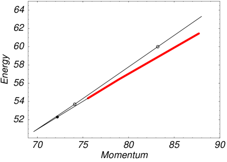
Figure 1: (Color online) The JR dispersion curve for the family of the axisymmetric solitary wave solutions. The part of the curve that corresponds to vortex rings is shown in grey (red). Three rarefaction waves that are considered in the text are indicated by circles.

The JR sequence can be uniquely characterised in other ways, for example by the velocity, $U$, of the wave or by min($u$), the minimum of the real part of $\psi=u+{\rm i}v$. Fig. 2 shows min($u$) as a function of $U$ for the entire family of JR solutions. In the limit $U\to 0$ of large vortex rings, min($u$) $\to-1$; in the opposite limit, $U\to c$, of large rarefaction waves, min($u$) $\to+1$. Between these extremes, the case min($u$) = 0 deserves special mention, as it separates the rarefaction waves, which do not possess vorticity, from the vortex-type solutions which do. In this case, $\psi$ vanishes at a single point, so that this solution might appropriately be termed a ‘point defect’; its velocity is approximately $U\approx 0.62$. The cusp ($U\approx 0.65$) in the $pE-$plot arises because $U=\partial E/\partial p=E^{\prime}(U)/p^{\prime}(U)$, so that extrema of $p$ are simultaneously extrema of $E$.

Figure 2: The minimum of the real part of the wavefunction, $Re(\psi)=u$, for the JR solitary waves as a function of velocity $U$. The open circle marks the point defect; closed circles show computed points through which the continuous line is drawn.

It was suggested in [3] as well as in its more detailed sequel [4] that every solitary wave on the upper branch is unstable, since it is energetically favourable for it to ‘collapse’ onto the lower branch of smaller energy at the same momentum. A Derrick-type argument [5] was used in which neighbouring axisymmetric states having the same $p$ as the upper branch solution to (1) were shown to have a smaller $E$. It would follow that the solution is unstable provided that $p$ and $E$ are the only quantities conserved by (1) in 3D, but this has never been demonstrated. Moreover, rarefaction waves on the upper branch of the JR dispersion curve are seen in numerical simulations: they evolve from a density depletion of a condensate [10] and appear during condensate formation from a strongly non-equilibrated Bose gas [14]. They may exist for a considerable time before they either collapse onto the lower branch of the JR dispersion curve or lose their energy to sound waves and disappear.

Evidently there is a paradox. On the one hand, if the assumption that $p$ and $E$ are the only conserved quantities in 3D is correct and the upper branch solutions are intrinsically unstable, how could they even form? On the other hand, if the assumption is false and the upper branch solutions are stable, why do they ultimately disappear? Is it because they are metastable or because they lose energy and momentum through collisions with other waves in the system?

The goal of this paper is to resolve this paradox. In Section 2, we demonstrate that the upper branch solitary waves are unstable. In Section 3.1, we show that, nevertheless, a perturbed solitary wave on the upper branch will generally evolve towards an unperturbed state on that branch and remain in its vicinity for a long period. Eventually, however, as illustrated in Section 3.2, it collapses onto the lower branch or disappears entirely. Another facet of such evolutionary processes is studied in Section 3.3, where it is shown how two rarefaction waves from the upper branch that move in the same direction can create a vortex ring. In Section 3.4 we demonstrate how unstable rarefaction waves can form from the evolution of a density depletion. We conclude in Section 4 with a brief summary of our findings.

2 Linear stability of the rarefaction solitary waves

2.1 The eigenvalue problem

In a reference frame moving with velocity $U$ in the $z-$direction, the GP equation (1) is

$$-2{\rm i}\,\partial_{t}\psi+2{\rm i}U\,\partial_{z}\psi=\nabla^{2}\psi+(1-|\psi|^{2})\psi,$$ (4)

solutions to which must obey

$$\psi\to 1,\qquad\mbox{for}\qquad r\equiv|{\bf x}|\to\infty\,.$$ (5)

The “basic solution” to (4) and (5) is the solitary wave, $\psi_{0}$ $(=u_{0}+{\rm i}v_{0})$, for which

$$2{\rm i}U\,\partial_{z}\psi_{0} = \nabla^{2}\psi_{0}+(1-|\psi_{0}|^{2})\psi_{0}\,,$$ (6)

$$\psi_{0} \to 1,\qquad\mbox{for}\qquad r\to\infty\,.$$ (7)

In this Section, we seek to determine the fate of small perturbations to $\psi_{0}$. We write

$$\psi({\bf x},t)=\psi_{0}({\bf x})+\widehat{\psi}({\bf x},t)\,.$$ (8)

On substituting (8) into (4) and linearising with respect to $\widehat{\psi}$, we find that

$$-2{\rm i}\partial_{t}\widehat{\psi}\,+\,2{\rm i}U\partial_{z}\widehat{\psi}\, = \,\nabla^{2}\widehat{\psi}\,+\,(1-2|\psi_{0}|^{2})\widehat{\psi}\,-\,\psi_{0}^{2}\widehat{\psi}^{*}\,,$$ (9)

$$\widehat{\psi} \to 0,\qquad\mbox{for}\qquad r\to\infty\,,$$ (10)

where $*$ stands for complex conjugation. Further discussion of (10) is postponed to §2.4. The objective now is the general solution of the initial value problem, i.e., the solution of (9) and (10), starting from an arbitrarily specified initial state. Following a well-trodden path in stability theory, we suppose that the solution can be expressed as a linear combination of a complete set of normal mode solutions. Alternative approaches to the initial value problem will be described in §3.

2.2 Real growth rates

Equation (9) admits normal mode solutions in which

$$\widehat{\psi}({\bf x},t)=p_{1}({\bf x})\mbox{e}^{\sigma t}\,,\qquad\widehat{\psi}^{*}({\bf x},t)=p^{*}_{2}({\bf x})\mbox{e}^{\sigma t}\,,$$ (11)

and

$$Lp_{1}-\psi_{0}^{2}p_{2}^{*}=-2{\rm i}\sigma p_{1}\,,\qquad L^{*}p_{2}^{*}-\psi_{0}^{*}{{}^{2}}p_{1}=\,\,2{\rm i}\sigma p^{*}_{2}\,,$$ (12)

where

$$L\,=\,\nabla^{2}\,+\,1\,-\,2|\psi_{0}|^{2}\,-\,2{\rm i}U\partial_{z}\,.$$ (13)

If the growth rate $\sigma$ is real, we may take

$$p_{1}=p_{2}=p=u+{\rm i}v\quad(\mbox{say})\,,$$ (14)

where $u$ and $v$ are real, both being proportional to $\cos m\phi$ or $\sin m\phi$ where $m$ is an integer and ($s$, $\phi$, $z$) are cylindrical coordinates. We shall be primarily interested in the axisymmetric case $m=0$. Equations (12) require

$$Lp-\psi_{0}^{2}p^{*}=-2{\rm i}\sigma p\,,$$ (15)

or equivalently

$$\nabla^{2}u+2U\partial_{z}v+(1-3u_{0}^{2}-v_{0}^{2})u-2u_{0}v_{0}v = \quad 2\sigma v\,,$$ (16)

$$\nabla^{2}v-2U\partial_{z}u+(1-u_{0}^{2}-3v_{0}^{2})v-2u_{0}v_{0}u = -2\sigma u\,,$$ (17)

$$u,v\quad\to 0,\quad\mbox{for}\quad r \to \infty\,,$$ (18)

where $\psi_{0}=u_{0}+{\rm i}v_{0}$.

The numerical solution of (16) – (18), was achieved by first making the change of independent variables suggested by [3]: $z^{\prime}=z$ and $s^{\prime}=s\surd(1-2U^{2})$. We mapped the infinite domain onto the box $(0,\textstyle{\frac{1}{2}}\pi)\times(-\textstyle{\frac{1}{2}}\pi,\textstyle{\frac{1}{2}}\pi)$ using the transformation

$$\widehat{z}=\tan^{-1}(Cz^{\prime}),$$ (19)

with a similar transformation for $s^{\prime}$; here $C$ ($\sim 0.4-0.5$) is a constant chosen at our convenience. We also write $\psi=\Psi+1$, so that the boundary conditions at infinity are $\Psi=0$.

We used the Newton-Raphson iteration procedure (using a banded matrix linear solver based on the bi-conjugate gradient stabilised iterative method with preconditioning) in the frame of reference moving with velocity $U$ to find solitary waves from solutions of

$$2{\rm i}UR\cos^{2}\widehat{z}\,\partial_{\widehat{z}}\Psi_{0} = {\cal L}\Psi_{0}-(\Psi_{0}+\Psi^{*}_{0}+|\Psi_{0}|^{2})(1+\Psi_{0}),$$

$${\rm and}\quad\Psi_{0} \to 0,\quad{\rm as}\quad s,\,z\to\infty,$$ (20)

where

$${\cal L}\! \!\!=\!\! \!R^{2}(1-2U^{2})\cos^{3}\widehat{s}\left[\cos\widehat{s}\,\frac{\partial^{2}}{\partial\widehat{s}^{2}}\!-\!\left(2\sin\widehat{s}-\frac{1}{\sin\widehat{s}}\right)\,\frac{\partial}{\partial\widehat{s}}\right]$$ (21)

$$+ R^{2}\cos^{3}\widehat{z}\left[\cos\widehat{z}\,\frac{\partial^{2}}{\partial\widehat{z}^{2}}\,-\,2\sin\widehat{z}\,\frac{\partial}{\partial\widehat{z}}\right]\,.$$

We also used (19) to transform (16) – (18). The resulting matrix equation was then discretised and gave the classic eigenvalue problem, $A{\bf x}=\sigma{\bf x}$, for $\sigma$. Eigenvalues can often be found successively by the Arnoldi/Lanczos process, in which the extreme eigenvalues are found first and the remaining eigenvalues are found successively by the ‘shift and invert’ technique, in which the original eigenvalue is shifted by $\lambda$ (say), and $A-\lambda I$ is inverted to transform the equation to $(A-\lambda I)^{-1}{\bf x}=\mu{\bf x}$, where $\mu=1/(\sigma-\lambda)$, so that the original eigenvalue is easily recovered as $\mu^{-1}+\lambda$. We employed the ARPACK [15] collection of subroutines, that uses the Implicitly Shifted QR technique that is suitable for large scale problems. The algorithm is designed to compute a few ($k$) eigenvalues with user specified features such as those of largest real part or largest magnitude. Storage requirements are on the order of $n*k$ locations, where $n$ is a number of columns of the matrix $A$. A set of Schur basis vectors for the desired $k$-dimensional eigenspace is computed which is numerically orthogonal to working precision.

The basic solution was found with a maximum resolution of 250$\times$200, making the real matrix generated by (16) – (17) of order $10^{5}\times 10^{5}$. The resolution of the basic solution was halved to check the accuracy of the eigenvalues found.

We found that $\sigma^{2}$ is real for all solutions of (16) – (18). To explain this, we first observe that we are interested only in perturbations that preserve the mass of the state $\psi_{0}$ in the sense that, if use (8) to evaluate the mass flux across any remote surface, ${\rm S}_{\infty}$, surrounding a volume $V_{\infty}$ containing and moving with the solitary wave, it is, to second order in $\widehat{\psi}$, the same as the mass flux implied by $\psi_{0}$. This implies that

$$\oint_{{\rm S}_{\infty}}[(\widehat{\psi}^{*}{\kern-0.24994pt\hbox{$\nabla$}\kern-8.33336pt\kern 0.50003pt\hbox{$\nabla$}\kern-8.33336pt\kern-0.24994pt\raise 0.43304pt\hbox{$\nabla$}}\widehat{\psi}-\widehat{\psi}{\kern-0.24994pt\hbox{$\nabla$}\kern-8.33336pt\kern 0.50003pt\hbox{$\nabla$}\kern-8.33336pt\kern-0.24994pt\raise 0.43304pt\hbox{$\nabla$}}\widehat{\psi}^{*})-2{\rm i}U|\widehat{\psi}|^{2}\widehat{\bf{z}}]\,{\kern-0.24994pt\hbox{$\cdot$}\kern-2.77779pt\kern 0.50003pt\hbox{$\cdot$}\kern-2.77779pt\kern-0.24994pt\raise 0.43304pt\hbox{$\cdot$}}\,{\bf dS}\,=\,0\,.$$ (22)

This in turn implies that the operator $L$ is hermitian:

$$\int_{V_{\infty}}\widehat{\psi}L^{*}\widehat{\psi}^{*}dV\,=\,\int_{V_{\infty}}\widehat{\psi}^{*}L\widehat{\psi}\,dV\,.$$ (23)

From this relation and (15), it follows that

$$\int_{V_{\infty}}\!\!\![|\,Lp|^{2}\,-\,\psi_{0}^{2}p^{*}L^{*}p^{*}]\,dV\!\!\! = \!\!\!-\!2{\rm i}\sigma\int_{V_{\infty}}\!\!\!\!pL^{*}p^{*}dV$$ (24)

$$= \!\!-2{\rm i}\sigma\int_{V_{\infty}}\!\!\!\!p^{*}Lp\,dV\,\!\!=\!\!-\,2{\rm i}\sigma\int_{V_{\infty}}\!\!\!\!p^{*}[\psi_{0}^{2}p^{*}-2{\rm i}\sigma p]\,dV.$$

Re-arranging this equation and using (15) again, we find that

$$\int_{V_{\infty}}\!\!\![|\,Lp|^{2}\,-|\psi_{0}|^{4}|p|^{2}]\,dV\,=\,-4\sigma^{2}\int_{V_{\infty}}\!\!\!|p|^{2}\,dV.$$ (25)

It follows that $\sigma^{2}$ can only take real values. The numerical results indicate that the eigenvalue spectrum is infinite and discrete and (25) shows that its limit point is at $\sigma^{2}=-\infty$. But only the necessarily finite number of positive $\sigma^{2}$ are relevant to the physical problem; see §2.3.

For the upper branch of the JR dispersion curve, we found only one family of convincingly positive $\sigma^{2}$, but this family (for which $m=0$) is sufficient to establish that the rarefaction waves are unstable to axisymmetric perturbations. The family seemed to disappear as the cusp $U=U_{c}$ was approached, and to become continuous with a family of negative $\sigma^{2}$ modes on the lower branch of the JR dispersion curve. Numerical work is incapable of establishing this fact unequivocally but an analytic argument given in Appendix A lends support. As $U\to c$, the growth rate of the instability tends to zero too (see Appendix B). One of the more striking results of the numerical work was the discovery that $\sigma$ is small everywhere on the upper branch. It was found that $\sigma$ has a single maximum $\sigma_{\rm max}(U)$, of approximately 0.012, attained for $U\sim 0.68$. The fact that $\sigma_{\rm max}(U)$ is so small means that the enfolding time on which the instability grows is long, being greater than 1/0.012 $\sim$ 84 in all cases. Fig. 3 shows the density and the phase contour plots of the wave function for the the fastest growing mode of perturbation for rarefaction solitary wave moving in the positive $z-$direction with the velocity $U=0.68$. Fig. 4 depicts the maximum growth rate $\sigma_{\rm max}(U)$ as a function of the rarefaction wave velocity, $U$.

No instabilities were discovered for the asymmetric ($m\neq 0$) modes on either branch of the JR dispersion curve, but the neutral $|m|=1$ modes, corresponding to infinitesimal displacement of the basic state in a direction perpendicular to O$z$, were located.

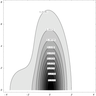
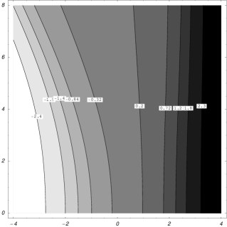
Figure 3: The density (a) and the phase (b) of the wave function for the the fastest growing mode of perturbation for rarefaction solitary wave moving in the positive $z-$direction with the velocity $U=0.68$. (These results were derived by solving the spectral problem (16) – (17) numerically).

      

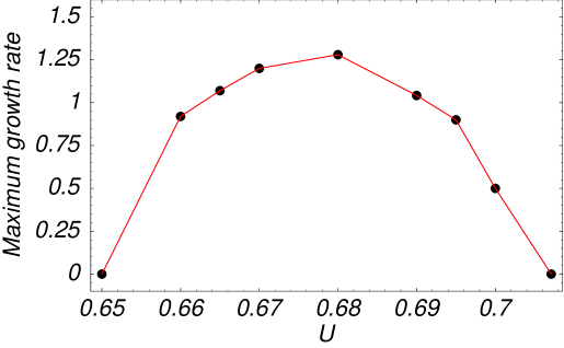
Figure 4: The maximum growth rate $\sigma_{\rm max}(U)$ as a function of the rarefaction wave velocity, $U$. (These results were derived by solving the spectral problem (16) – (17) numerically).

2.3 Complex growth rates

When $\sigma$ is complex, the complex conjugate of either of (11) contradicts the other. On making the exchange $1\leftrightarrow 2$ and taking the complex conjugates of both equations (12), we see however that, if $\sigma$ is an eigenvalue, so is $\sigma^{*}$. Thus solutions to (9) exist of the form

$$\widehat{\psi}({\bf x},t)=p_{1}({\bf x})\mbox{e}^{\sigma t}+p_{2}({\bf x})\mbox{e}^{\sigma^{*}t}\,,\qquad\widehat{\psi}^{*}({\bf x},t)=p^{*}_{2}({\bf x})\mbox{e}^{\sigma t}+p^{*}_{1}({\bf x})\mbox{e}^{\sigma^{*}t}\,.$$ (26)

By making use of the Hermitian property of $L$, it follows from an argument similar to the one that led to (25) that

$$\int[|Lp_{1}|^{2}-|\psi_{0}|^{4}|p_{1}|^{2}-\psi_{0}^{2}(p_{2}^{*}L^{*}p_{1}^{*}-p_{1}^{*}L^{*}p_{2}^{*})]dV\!\! = \!\!-4\sigma^{2}\int|p_{1}|^{2}dV\,,$$ (27)

$$\int[|Lp_{2}|^{2}-|\psi_{0}|^{4}|p_{2}|^{2}-\psi_{0}^{*2}(p_{1}Lp_{2}-p_{2}Lp_{1})]dV\!\! = \!\!-4\sigma^{2}\int|p_{2}|^{2}dV\,.$$ (28)

On subtracting corresponding sides of these equations we obtain

$$4\sigma^{2}\int[|p_{2}|^{2}-|p_{1}|^{2}]dV\!\! = \!\!\int[|Lp_{1}|^{2}-|Lp_{2}|^{2}-|\psi_{0}|^{4}(|p_{1}|^{2}-|p_{2}|^{2})$$ (29)

$$+ \!\!\psi_{0}^{*2}(p_{1}Lp_{2}-p_{2}Lp_{1})+\psi_{0}^{2}(p_{1}^{*}L^{*}p_{2}^{*}-p_{2}^{*}L^{*}p_{1}^{*})]dV\,.$$

In what follows, we shall assume that there are no eigenvalues (apart from the real $\sigma$ of §2.1) for which

$$\int|p_{1}|^{2}dV = \int|p_{2}|^{2}dV\,,$$ (30)

$$\int[|Lp_{1}|^{2}-|Lp_{2}|^{2}-|\psi_{0}|^{4}(|p_{1}|^{2}\!\! - \!\!|p_{2}|^{2})$$

$$+\psi_{0}^{*2}(p_{1}Lp_{2}-p_{2}Lp_{1}) + \psi_{0}^{2}(p_{1}^{*}L^{*}p_{2}^{*}-p_{2}^{*}L^{*}p_{1}^{*})]dV=0\,.$$ (31)

hold simultaneously. It then follows from (29) that $\sigma^{2}$ is real. Therefore the only eigenvalues that are complex are purely imaginary. The main import of this result is that §2.2 has already located all modes that can become unstable.

For modes with imaginary $\sigma={\rm i}\omega$, we substitute

$$p_{1}=u_{1}+{\rm i}v_{1},\qquad p_{2}=u_{2}+{\rm i}v_{2}\,,$$ (32)

into (12) to obtain an 8^th order system that replaces the 4^th order system (16) and (17):

$$Mu_{1}+2U\partial_{z}v_{1}-(u_{0}^{2}-v_{0}^{2})u_{2}-2u_{0}v_{0}v_{2} = \quad 2\omega u_{1}\,,$$ (33)

$$Mv_{1}-2U\partial_{z}u_{1}+(u_{0}^{2}-v_{0}^{2})v_{2}-2u_{0}v_{0}u_{2} = \quad 2\omega v_{1}\,,$$ (34)

$$Mu_{2}+2U\partial_{z}v_{2}-(u_{0}^{2}-v_{0}^{2})u_{1}-2u_{0}v_{0}v_{1} = -2\omega u_{2}\,,$$ (35)

$$Mv_{2}-2U\partial_{z}u_{2}+(u_{0}^{2}-v_{0}^{2})v_{1}-2u_{0}v_{0}u_{1} = -2\omega v_{2}\,,$$ (36)

where

$$M=\nabla^{2}+1-2u_{0}^{2}-2v_{0}^{2}\,.$$ (37)

2.4 Large $r$ behaviour

It might seem that (10) is the obvious and correct boundary condition to apply to solutions of (9), but there are some subtleties. Consider first the solutions developed in §2.3. For $r\to\infty$, $u_{1}$ and $v_{1}$ make contributions to $\widehat{\psi}$ that are dominantly proportional to

$$r^{-1}\exp[i(kr+\omega t)]\,.$$ (38)

Since $u_{0}-1$ = O($r^{-3}$) and $v_{0}$ = O($r^{-2}$), the possible values of $k$ implied by (33) – (36) are:

$$\omega\pm wk=\pm\textstyle{\frac{1}{2}}k\surd(k^{2}+2)\,,$$ (39)

where $w=Uz/r$ ($-1/\sqrt{2}<w<1/\sqrt{2}$). The eigenfunction is a linear combination therefore of 8 solutions of the form (38), for the 8 roots of the 2 quartic equations

$$k^{4}+2(1-2w^{2})k^{2}\pm 8\omega wk-4\omega^{2}=0\,.$$ (40)

It is easily shown that 4 of these roots are real; 2 are positive and 2 negative. These correspond to ingoing and outgoing sound waves. They satisfy the requirement (10), but they do not obey the condition (22) needed to establish that $L$ is self-adjoint. This difficulty can be surmounted however by requiring that the waves are reflected from S_∞. A more serious issue concerns the remaining 4 complex roots of (40), two of which have positive real parts and two negative. To satisfy (10), the eigenfunction must exclude the two roots for which Im($k$) $<$ 0, irrespective of whether the remaining $k$ correspond to ingoing or outgoing energy flux.

In short, hidden in the succinct statement (10), are physical requirements on the eigenfunctions that are far from obvious and may be controversial. The same is true in the case of real $\sigma$ considered in §2.2. For this reason, and also to throw further light on the evolution of perturbations to the basic state, it was thought desirable to carry out the numerical experiments reported in §3 below. These attack the initial value problem without preconceptions such as (10), and without the necessity of supposing that the perturbation to $\psi_{0}$ is infinitesimal.

3 Numerical simulations involving rarefaction waves

In this section we shall report on numerical solutions of the GP equation (4) that show that the solitary waves on the upper branch can, despite their instability, be surprisingly robust, but that nevertheless they eventually evolve onto the lower branch.

3.1 Perturbed unstable solitary wave

Starting with a rarefaction solitary wave from the upper branch of the JP dispersion curve, we consider perturbations of the form

$$\psi({\bf x},t=0)=\psi_{0}({\bf x})+{\cal N}({\bf x}),\quad\mbox{\rm where}\quad{\cal N}=\sum_{\bf k}a_{\bf k}\exp(i{\bf k\cdot x})\,.$$ (41)

Here $\cal N$ corresponds to the state of a weakly interacting Bose gas in the kinetic regime [6]; the phases of the complex amplitudes $a_{\bf k}$ are distributed randomly. To make the disturbance decay to zero far from the solitary wave and to give it both axisymmetric and non-axisymmetric components, we take

$${\cal N}(x,y,z) = \frac{1}{M^{3}}\sum_{{\bf k}=(l,m,n)}^{M}a_{\bf k}\exp\biggr{[}i\frac{\pi}{10}\Bigr{(}lx+\frac{my}{\sqrt{2}}+\frac{nz}{\sqrt{3}}\Bigl{)}\biggl{]}$$ (42)

$$\times \exp[-0.01(x^{2}+2y^{2}+3z^{2})].$$

The maximum frequency, $M$, and the modulus of the complex amplitude $|a_{\bf k}|$ are two parameters that we vary.

In what follows we say that a perturbed solution evolves to a JR solitary wave of velocity $U$ if, in a sufficiently large neighbourhood of its centre and for a significant period of time, it becomes and remains axisymmetric and form-preserving to good accuracy, and if in addition its minimum $u$ corresponds to the $U$ shown in Fig. 2. By “a significant period”, we mean an elapsed time exceeding 10, by “good accuracy”, we mean that the density deviations do not exceed 0.01 and, by “a sufficiently large neighbourhood”, we mean within a sphere of radius 20 surrounding the origin.

We performed numerical integrations of (20) with the time derivative $-2{\rm i}\partial_{t}\Psi$ restored to the left-hand side. Since the integration was terminated at a finite time $t$, before sound waves from the disturbance can reach $r=\infty$, the boundary condition (10) on $\widehat{\psi}$ is irrelevant. We employed the same mapping as in §2.2. We used fourth order finite differences in space except for second order finite differences at the boundary, and fourth order Runge-Kutta integration in time. The initial state at $t=0$ was given by (41) – (42), where $\psi_{0}({\bf x})$ are rarefaction waves from the upper branch of the JR dispersion curve. We principally focused on two cases: $U=0.68$ and $U=0.69$; see Fig. 1.

In each case, our simulations show that, for $5\leq M\leq 20$ and $|a_{\bf k}|\leq 4$, the wave has, by $t\sim 20$, rid itself of the perturbation, apparently by acoustic radiation, and has returned to the vicinity of the upper branch, though with a velocity that is slightly smaller (by 1% or less) than that of the initial $\psi_{0}$ in (41). Fig. 5 shows snapshots of the evolution of the rarefaction waves for $U=0.68$ and $U=0.69$, for the initial perturbation (41) – (42) with $M=20$ and $|a_{\bf k}|=2$. By $t=18$, each solution had evolved close to an unperturbed rarefaction wave, and at $t=36$ it still remains in its vicinity. On a longer time scale ($t>100$), the rarefaction waves either lose their energy and momentum to sound or collapse onto the lower branch of the JR dispersion curve.

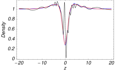
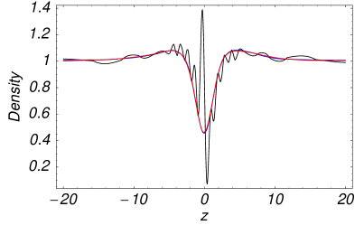
Figure 5: (Colour online) Snapshots at $t=0$ (black line), $t=18$ (dark grey or blue line) and $t=36$ (light grey or red line) of the density of the condensate along the direction of the motion. Here $|\psi(0,0,z)|^{2}$ was obtained by numerically integrating the GP model (1) for the perturbed rarefaction waves.

3.2 Evolution of unstable rarefaction waves into vortex rings

In [7] an algorithm was developed for generalised rational approximations to the JR solitary waves having the correct asymptotic behaviour at infinity. An axisymmetric solitary wave moving with velocity $U$ along the $z-$axis is well approximated by $\psi(s,z)=1+u(s,z)+{\rm i}\,v(s,z)$ where

$$u = \frac{a_{00}+a_{10}{z^{\prime}}^{2}+a_{01}s^{2}+mc_{20}^{7/4}U(2{z^{\prime}}^{2}-f(U)s^{2})({z^{\prime}}^{2}+f(U)s^{2})}{(1+c_{10}{z^{\prime}}^{2}+c_{01}s^{2}+c_{20}({z^{\prime}}^{2}+f(U)s^{2})^{2})^{7/4}},$$

$$v = z^{\prime}\frac{b_{00}+b_{10}{z^{\prime}}^{2}+b_{01}s^{2}-mc_{20}^{7/4}({z^{\prime}}^{2}+f(U)s^{2})^{2}}{(1+c_{10}{z^{\prime}}^{2}+c_{01}s^{2}+c_{20}({z^{\prime}}^{2}+f(U)s^{2})^{2})^{7/4}},$$ (43)

where $z^{\prime}=z-Ut$ and $f(U)=1-2U^{2}$. Here $a_{ij}$, $b_{ij}$, $c_{ij}$ and the dipole moment $m$ are functions of $U$ determined by series expansions. For example, the rarefaction wave $U=0.69$ is given by

$$\!\!u\!\! \!=\Bigl{(}-0.2779\!-\!0.00182{z^{\prime}}^{2}\!-\!0.00128\,s^{2}\!+\!0.00035(2{z^{\prime}}^{2}\!-\!0.0478s^{2})({z^{\prime}}^{2}\!+\!0.0478s^{2})\Bigr{)}\!\mathchar 4878\relax\!{\cal D}\,,$$ (44)

$$\!\!v\!\! \!=z^{\prime}\Bigl{(}-0.34761\!-\!0.02198{z^{\prime}}^{2}\!-\!0.00262s^{2}\!-\!0.00051({z^{\prime}}^{2}\!+\!0.0478s^{2})^{2}\Bigr{)}\!\mathchar 4878\relax\!{\cal D}\,,$$

where

$${\cal D}=\Bigr{(}1+0.11749\,{z^{\prime}}^{2}+0.01470\,s^{2}+0.00356({z^{\prime}}^{2}+0.0478\,s^{2})^{2}\Bigl{)}^{7/4}\,.$$ (45)

By (2) and (3), the momentum and energy are

$$p = {2\pi}\int(uv_{x}-vu_{x})s\,ds\,dx\,,$$ (46)

$${\cal E} = \pi\int[u_{z}^{2}+u_{s}^{2}+v_{z}^{2}+v_{s}^{2}-\tfrac{1}{2}(2u+u^{2}+v^{2})^{2}]s\,ds\,dx\,,$$ (47)

where $u_{z}=\partial u/\partial z$, $u_{s}=\partial u/\partial s$, etc. By substituting the approximation (44) into (46) and (47), we obtain $p\approx 84.15$ and ${\cal E}\approx 61.2$; these may be compared with the values $p\approx 83.2$ and ${\cal E}\approx 60.0$ obtained by from direct integration of (6). The maximum residual error, calculated as the global maximum of the square of the error amplitude [see (29) of [7]] is $\sim 0.003$. Evidently, (44) provides a starting point that is very close to the upper branch.

To follow the evolution of (44) over long times, we performed a numerical integration of (1), using a finite differences scheme with open boundaries to allow sound waves to escape (see our previous work [8] or [9] for a detailed description of the numerical method). The computational box has dimensions $D^{3}=100^{3}$, the space discretization was $dx=dy=dz=0.5$, and the time step was $dt=0.1/(dx^{2}+dy^{2}+dz^{2})$. The small initial deviation of (44) from the upper branch grows with time, and the solution slowly evolves into a vortex ring. Fig. 6 illustrates this process. Circulation is acquired at $t\sim 148$ and a well-formed vortex ring emerges by $t\sim 160$.

Figure 6: (Colour online) Snapshots of the contour plots of the density cross-section of a condensate, obtained by numerically integrating the GP model (1). The initial condition was $\psi=1+u+{\rm i}v$, with $u$ and $v$ given by (44). Black dashed lines show zeros of the real and imaginary parts of $\psi$ at $t>0$. Their intersection therefore shows the position of topological zeros. Both low and high density regions are shown in darker shades so that regions of intermediate density are emphasised. Only a portion of an actual computational box is shown.

3.3 Vortex nucleation resulting from the interaction of rarefaction waves

In [7] we considered the evolution of two identical rarefaction waves ($U=0.63$) from the lower branch. These were centred on the $z-$axis, and moved along it, one behind the other. It was found that the trailing wave transfered part of its energy and momentum to the leading wave, until eventually the latter became a vortex ring. We now consider an analogous situation but one in which both rarefaction waves initially lie on the upper branch. We numerically integrated (1) in the frame of reference moving with $U=0.69$, taking the initial state to be $\psi(t=0)=\psi_{0}(x-5,s)\psi_{0}(x+5,s)$, where $\psi_{0}(x,s)$ is defined by (44). Fig. 7 shows snapshots of the subsequent evolution. This is very different from the evolution of the two rarefaction waves from the lower branch, although there is again a transfer of energy and momentum from the trailing wave to the leading wave. The leading wave does not, however, evolve to a higher energy state on the upper branch but instead slowly transforms itself into a vortex ring on the lower branch. Apparently, the transfer of energy and momentum from the trailing vortex is insufficient to carry the wave to a higher energy state on the upper branch; it remains ‘beneath’ that branch and can therefore only evolve onto the lower branch; see Fig. 1).

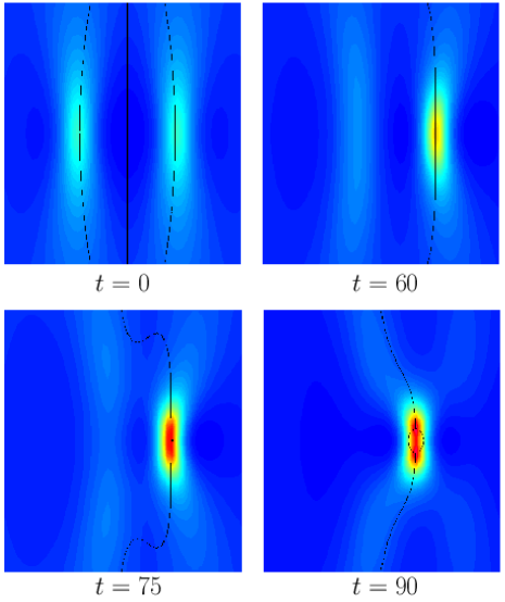
Figure 7: (Colour online) Snapshots of the contour plots of the density cross-section of a condensate, obtained by numerically integrating the GP model (1). The initial condition was $\psi(t=0)=\psi_{0}(x-5,s)\psi_{0}(x+5,s)$, given by (44) where $\psi_{0}=1+u+{\rm i}v$. Black dashed lines show zeros of the real and imaginary parts of $\psi$. Their intersection therefore shows the position of topological zeros. Both low and high density regions are shown in darker shades so that regions of intermediate density are emphasised. Only a portion of an actual computational box is shown.

3.4 Evolution of the density depletions in condensates

There are several ways of creating rarefaction waves in a condensate, that make use of some of the methods described in [10]. A tangle of vortices is created when angular momentum is transmitted to the condensate by rotationally stirring it with a laser beam [11]. In addition to vortices, such stirring creates many local depletions in the condensate density. It was shown in [10] that such depletions are unstable and generate both vortices and rarefaction waves. We shall now show that, by creating a shallow ellipsoidal depletion in condensate density, it is possible to generate rarefaction waves alone on the upper branch of the JR dispersion curve .

We numerically integrated (1) taking as our starting point a spheroidal depletion of condensate:

$$\psi({\bf x},0)=\tfrac{1}{2}+\tfrac{1}{2}\tanh\left[0.01(z^{2}+0.5s^{2}-36)\right].$$ (48)

The minimum amplitude of the initial state is $0.33$, at the origin. After the condensate fills the cavity, it begins to expand, its density oscillating around the unperturbed state $\psi=1$. These depressions in density are unstable, in a manner similar to the instability of Kadomtsev-Petviashvili 2D solitons in 3D [12]. This results in the creation of two rarefaction waves moving outwards in opposite directions. Fig. 8 shows snapshots of the density in the $z=0$ cross-section. Well-defined vorticity-free localised axisymmetric disturbances – rarefaction waves — are formed at around $t\sim 30$. Their axes of symmetry lie on Im$(\psi)=v({\bf x},t)=0$ and are plotted as solid lines in the $t=33$ snapshot.

Various stages in the collapse of a stationary spherically symmetric bubble were elucidated in [13], where conditions necessary for vortex nucleation were also established. A similar analysis applies to the evolution of the density depletion (48), for which the density is everywhere nonzero initially. In particular, it would be possible to calculate the critical radius of a spherical depletion, as a function of minimum density, for rarefaction waves to be nucleated.

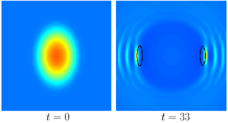
Figure 8: (Colour online) Snapshots of the contour plots of the density cross-section of a condensate obtained by numerically integrating the GP model (1) starting from the spheroidal density depletion (48). Black solid lines show zeros imaginary parts of $\psi$, the straight segment being the axis of symmetry of the rarefaction wave. Both low and high density regions are shown in darker shades so that regions of intermediate density are emphasised.

4 Conclusions

We have analysed the linear stability problem for solitary waves of the GP equation. We have shown that the rarefaction solitary waves on the upper branch of the JR dispersion curve are unstable to infinitesimal perturbations and we have calculated the maximum growth rate, and found it to be small, being approximately $\sigma_{\rm max}=\sqrt{2}\times 0.012c/\xi\approx 70$ ${\rm s}^{-1}$ (taking the healing length $\xi=0.7\mu$m and the Bogoliubov speed of sound $c=2.8$ mm s^-1 as in NIST experiments [2]). Our results indicate that the solitary waves on the lower branch and all two-dimensional solitary waves are linearly stable. By numerically integrating the GP equation, we studied the properties of the unstable solitary waves and, in particular, we showed that the system tends to remain close to the unstable solution, spending a significant amount of time, of the order of a few multiples of $\tau_{\rm min}=1/\sigma_{\rm max}$, in its vicinity. Ultimately however it collapsed onto the lower branch or broke up into sound waves.

These conclusions suggest that rarefaction solitary waves could be experimentally detected and and studied in Bose condensates alongside the vortex rings. They can be created by laser beams and evolve from a local depletion of the condensate. Rarefaction waves will also appear as the result of the self-evolution of a strongly nonequilibrated Bose gas [14]. Like the vortex rings, they can in principle be observed in expanding condensates.

5 Acknowledgements

The authors are grateful for support from NSF grant DMS-0104288. NGB thanks Professor Chris Jones for a useful discussion, Dr Paul Metcalfe for his help with installing and testing ARPACK, and Dr Jeroen Molemaker for a useful subroutine.

Appendix A: Eigenvalues at the cusp

It was argued in §2.1 that, for every $U$, the spectrum of $\sigma^{2}$, where $\sigma$ is the growth rate of perturbations is real, discrete and infinite, with limit point at $\sigma^{2}=-\infty$, i.e., only a finite number of positive $\sigma^{2}$ can exist for each $m$. The largest of these is the most significant since, when positive, it gives the largest growth rate for instability. Our numerical work strongly suggested that this $\sigma^{2}$ is part of the spectrum for the axisymmetric mode and that it changes sign precisely at the cusp, $U=U_{c}$, being positive for $U>U_{c}$ and negative for $U<U_{c}$. The aim of this Appendix is to re-enforce this conclusion by showing analytically that this $\sigma^{2}$ can change sign only at the cusp. The argument is analogous to one presented by Kuznetsov and Rasmussen [17] for 2D solitary waves.

In the axisymmetric case ($m=0$), (15) always possesses a neutral solution ($\sigma=0$) corresponding to an infinitesimal displacement of $\psi_{0}$ in the $z-$direction; we write this as

$$p^{(0)}=\partial\psi_{0}/\partial z\,.$$ (49)

We now seek a neighbouring solution for which $\sigma$ is small, vanishing when a double root of $\sigma$ exists. We expand this solution as

$$p=p^{(0)}+\sigma p^{(1)}+\sigma^{2}p^{(2)}+\dots\,.$$ (50)

Substituting (50) into (15), we obtain

$$Lp^{(0)}-\psi_{0}^{2}p^{(0)*}=0,$$ (51)

$$Lp^{(1)}-\psi_{0}^{2}p^{(1)*}=-2{\rm i}p^{(0)},$$ (52)

$$Lp^{(2)}-\psi_{0}^{2}p^{(2)*}=-2{\rm i}p^{(1)}.$$ (53)

The differential of (15) with respect to $U$ and (49) show that the solution to (52) is

$$p^{(1)}=-\partial\psi_{0}/\partial U.$$ (54)

A consistency condition follows from (53). It is easily seen, from (13) and (51) and the condition (10) on $\widehat{\psi}$ at infinity, that

$$\int\left[p^{(0)*}(Lp^{(2)}-\psi_{0}^{2}p^{(2)*})+p^{(0)}(L^{*}p^{(2)*}-\psi_{0}^{2}p^{(2)})\right]\,dV=0.$$ (55)

It now follows from (53) that

$$\frac{dp}{dU}\equiv\frac{1}{\rm i}\int\left(\frac{\partial\psi_{0}^{*}}{\partial z}\,\frac{\partial\psi_{0}}{\partial U}-\frac{\partial\psi_{0}}{\partial z}\,\frac{\partial\psi_{0}^{*}}{\partial U}\right)\,dV=0.$$ (56)

The left-hand equality here is established by differentiating (2) with respect to $U$ and carrying out integrations by parts.

It follows from (56) that the double zero of $\sigma$ can occur only at the cusp, the only point on the JR dispersion curve where $p^{\prime}(U)$ is zero.

Appendix B: The Gross-Pitaevskii equation for $U\to c$

In multidimensions the density depletion of the solitary rarefaction wave as well as the characteristic inverse length along the axis of propagation tend to zero as the solitary wave velocity, $U$, approaches the speed of sound, $c$. This allows us to reduce the GP equation to the Kadomtsev-Petviashvili type I (KPI) equation, that describes the propagation of acoustic waves of small amplitude and positive dispersion.

In [3] such a reduction was obtained as a compatibility condition of the equations written to $O(\epsilon^{4})$ where the small parameter $\epsilon\sim\surd(c-U)$. In what follows we derive the eigenvalue problem of the GP equation in the limit of $U\rightarrow c$ and show that it coincides with the eigenvalue problem for the KPI equation for an appropriate scaling of the eigenvalues.

We start by separating the real and imaginary parts of the basic state as $\psi_{0}=u_{0}+{\rm i}v_{0}$ and of the perturbation as $\widehat{\psi}=u+{\rm i}v$; see Section 2. The basic solution satisfies (6) so that

$$\nabla^{2}u_{0}+(1-u_{0}^{2}-v_{0}^{2})u_{0}+2U\partial_{z}v_{0}=0,\quad\nabla^{2}v_{0}+(1-u_{0}^{2}-v_{0}^{2})v_{0}-2U\partial_{z}u_{0}=0,$$ (57)

while $u$ and $v$ satisfy (16) – (17) where, without loss of generality, we take $m=0$. To make the reduction to the KPI equation we write

$$z\rightarrow z/\epsilon,\quad s\rightarrow s/\epsilon^{2},\qquad\mbox{\rm so that}\qquad\partial_{z}\rightarrow\epsilon\partial_{z},\quad\nabla^{2}\rightarrow\epsilon^{2}\partial^{2}z+\epsilon^{4}\nabla^{2}_{H},$$ (58)

where $\nabla^{2}_{H}=\partial^{2}_{s}+s^{-1}\partial_{s}$. Next we make the transformation

$$u_{0}\rightarrow 1+\epsilon^{2}u_{0},\quad v_{0}\rightarrow\epsilon v_{0},\quad u\rightarrow\epsilon u,\quad v\rightarrow v,\quad U\rightarrow c+\epsilon^{2}U,\quad\sigma\rightarrow\epsilon^{3}\sigma.$$ (59)

Note that the transformation of the eigenvalue $\sigma$ defines a slow timescale, the only one that makes the time-dependent GP equation consistent with the time-dependent KPI equation; see below.

The equations governing the basic solution and the perturbations become

$$\partial_{z}v_{0}-\sqrt{2}u_{0}-\frac{1}{\sqrt{2}}v_{0}^{2}+\frac{\epsilon^{2}}{\sqrt{2}}\biggl{[}\partial_{z}^{2}u_{0}-(3u_{0}+v_{0}^{2})u_{0}+2U\partial_{z}v_{0}\biggr{]}+O(\epsilon^{4})=0,$$ (60)

$$\partial_{z}^{2}v_{0}-\sqrt{2}\partial_{z}u_{0}-(2u_{0}+v_{0}^{2})v_{0}+\epsilon^{2}\biggl{[}\nabla^{2}_{H}v_{0}-u_{0}^{2}v_{0}-2U\partial_{z}u_{0}\biggr{]}+O(\epsilon^{4})=0,$$ (61)

$$\partial_{z}v-\sqrt{2}(u+v_{0}v)+\frac{\epsilon^{2}}{\sqrt{2}}\biggl{[}\partial_{z}^{2}u-(6u_{0}+v_{0}^{2})u-2u_{0}v_{0}v+2U\partial_{z}v-2\sigma v\biggr{]}+O(\epsilon^{4})=0,$$ (62)

$$\partial_{z}^{2}v-\sqrt{2}\partial_{z}u-(2u_{0}+3v_{0}^{2})v-2v_{0}u$$

$$\hskip 40.0pt+\epsilon^{2}\biggl{[}\nabla^{2}_{H}v-u_{0}^{2}v-2u_{0}v_{0}u-2U\partial_{z}u+2\sigma u\biggr{]}+O(\epsilon^{4})=0.$$

(63)

Now we expand all functions and the velocity $U$ in powers of $\epsilon^{2}$ as $u_{0}=u_{0}^{0}+\epsilon^{2}u_{0}^{1}$, etc. At leading order, (60) – (63) give

$$\partial_{z}v_{0}^{0}-\sqrt{2}u_{0}^{0}-\frac{1}{\sqrt{2}}v_{0}^{02}=0,$$ (64)

$$\partial_{z}^{2}v_{0}^{0}-\sqrt{2}\partial_{z}u_{0}^{0}-(2u_{0}^{0}+v_{0}^{02})v_{0}^{0}=0,$$ (65)

$$\partial_{z}v^{0}-\sqrt{2}u^{0}-\sqrt{2}v_{0}^{0}v^{0}=0,$$ (66)

$$\partial_{z}^{2}v^{0}-\sqrt{2}\partial_{z}u^{0}-(2u_{0}^{0}+3v_{0}^{02})v^{0}-2v_{0}^{0}u^{0}=0.$$ (67)

We first consider (64) – (65) and notice that (64) implies (65), so that

$$u_{0}^{0}=\frac{1}{\sqrt{2}}\partial_{z}v_{0}^{0}-\frac{1}{2}v_{0}^{02}.$$ (68)

We use (68) to eliminate $u_{0}^{0}$ from the leading order expressions in square brackets in (60) and (61) which we denote by $R$ and $S$ respectively. After making simplifications we obtain

$$R \equiv \partial_{z}^{2}u_{0}^{0}-(3u_{0}^{0}+v_{0}^{02})u_{0}^{0}+2U^{0}\partial_{z}v_{0}^{0}$$ (69)

$$= \frac{1}{\sqrt{2}}\partial_{z}^{3}v_{0}^{0}-v_{0}^{0}\partial_{z}^{2}v_{0}^{0}-\frac{5}{2}\Bigl{(}\partial_{z}v_{0}^{0}\Bigr{)}^{2}+\sqrt{2}v_{0}^{02}\partial_{z}v_{0}^{0}-\frac{1}{4}v_{0}^{04}+2U^{0}\partial_{z}v_{0}^{0}\,,$$

$$S \equiv \nabla^{2}_{H}v_{0}^{0}-u_{0}^{02}v_{0}^{0}-2U^{0}\partial_{z}u_{0}^{0}$$ (70)

$$= \nabla^{2}_{H}v_{0}^{0}-\biggl{(}\frac{1}{\sqrt{2}}\partial_{z}v_{0}^{0}-\frac{1}{2}v_{0}^{02}\biggr{)}^{2}\!\!v_{0}^{0}-2U^{0}\biggl{(}\frac{1}{\sqrt{2}}\partial_{z}^{2}v_{0}^{0}-v_{0}^{0}\partial_{z}v_{0}^{0}\biggr{)}.$$

Equations (60) – (61) become

$$\partial_{z}v_{0}^{1}-\sqrt{2}u_{0}^{1}-\sqrt{2}v_{0}^{0}v_{0}^{1}=-\frac{1}{\sqrt{2}}R,$$ (71)

$$\partial_{z}^{2}v_{0}^{1}-\sqrt{2}\partial_{z}u_{0}^{1}-(2u_{0}^{0}+3v_{0}^{02})v_{0}^{1}-2v_{0}^{0}u_{0}^{1}=-S.$$ (72)

The compatibility of (71) and (72) implies

$$S=\frac{1}{\sqrt{2}}\partial_{z}R+v_{0}^{0}R,$$ (73)

which is the KPI equation as derived in [3]:

$$2\sqrt{2}U^{0}\partial_{z}^{2}v_{0}^{0}-\nabla^{2}_{H}v_{0}^{0}+\partial_{z}\biggl{[}\frac{1}{2}\partial_{z}^{3}v_{0}^{0}-\frac{3}{\sqrt{2}}\biggl{(}\partial_{z}v_{0}^{0}\biggr{)}^{2}\biggr{]}=0\,.$$ (74)

Next we consider (62) and (63). At the leading order both (66) and (67) require that

$$u^{0}=\frac{1}{\sqrt{2}}\partial_{z}v^{0}-v_{0}^{0}v^{0}.$$ (75)

Note that, if we had assumed a different scaling for $\sigma$, we would now face an inconsistency. For example, if we had adopted $\sigma=O(\epsilon)$, we would have found at this point in the argument that $\sigma=0$, i.e., that $\sigma$ is asymptotically smaller than the assumed $O(\epsilon)$.

At the next order beyond (66) and (67), expressions $R^{\prime}$ and $S^{\prime}$ analogous to $R$ and $S$ arise:

$$R^{\prime}=\frac{\partial^{2}u^{0}}{\partial z^{2}}-(6u_{0}^{0}+v_{0}^{02})u^{0}-2u_{0}^{0}v_{0}^{0}v^{0}+2U^{0}\partial_{z}v^{0}-2\sigma v^{0}+2v_{0}^{1}v^{0},$$ (76)

$$S^{\prime}=\nabla^{2}_{H}v^{0}-u_{0}^{02}v^{0}-2u_{0}^{0}v_{0}^{0}u^{0}-2U^{0}\partial_{z}u^{0}+2\sigma u^{0}+(2u_{0}^{1}+6v_{0}^{0}v_{0}^{1})v^{0}+2v_{0}^{1}u^{0}.$$ (77)

We use (68) and (75) to eliminate $u_{0}^{0}$ and $u^{0}$ from (76) and (77). The equations (66) and (67) then have the form

$$\partial_{z}v^{1}-\sqrt{2}(v^{1}+v_{0}^{0}v^{1})=-\frac{1}{\sqrt{2}}R^{\prime},$$ (78)

$$\partial_{z}^{2}v^{1}-\sqrt{2}\partial_{z}u^{1}-(2u_{0}^{0}+3v_{0}^{02})v^{1}-2v_{0}^{0}u^{1}=-S^{\prime},$$ (79)

and the compatibility of (78) and (79) leads to the eigenvalue problem

$$S^{\prime}=\frac{1}{\sqrt{2}}\partial_{z}R^{\prime}+v_{0}^{0}R^{\prime},$$ (80)

or, after simplification,

$$2\sqrt{2}U^{0}\partial_{z}^{2}v^{1}-3\sqrt{2}\partial_{z}[\partial_{z}v_{0}^{0}\partial_{z}v^{1}]+\frac{1}{2}\partial_{z}^{4}v^{1}-\nabla^{2}_{H}v^{1}=2\sqrt{2}\sigma\partial_{z}v^{1}.$$ (81)

Notice, the spectral problem (81) is the same one as obtained from (74) written in time-dependent form as

$$\partial_{z}\biggl{[}2\sqrt{2}\partial_{t}V-2\sqrt{2}U^{0}\partial_{z}V+\frac{3}{\sqrt{2}}(\partial_{z}V)^{2}-\frac{1}{2}\partial_{z}^{3}V\biggr{]}+\nabla^{2}_{H}V=0,$$ (82)

where $V=v_{0}^{0}+v^{1}\exp(\sigma t)$. This proves that the KPI equation and the GP equation share the same linear stability properties, the eigenvalues being related by $\sigma_{KP}(c-U_{GP})^{3/2}=\sigma_{GP}$ as $U_{GP}\rightarrow c$.

References

• [1] Fetter A L and Svidzinsky A A 2001 J. Phys.: Condens. Matter 13 R135
• [2] Denschlag J, Simsarian J E, Feder D L et al 2000 Science 287 97
• [3] Jones C A and Roberts P H 1982 J. Phys. A: Gen. Phys. 15 2599
• [4] Jones C A, Putterman S J and Roberts P H 1986 J Phys A: Math Gen 19 2991
• [5] Derrick D H 1964 J. Math. Phys. 5 1252
• [6] Kagan Yu and Svistunov B V 1997 Phys. Rev. Lett. 79, 3331
• [7] Berloff N G 2004 J. Phys.: Math. Gen. 37, 1617
• [8] Berloff N G and Roberts P H 2000 J. Phys. A: Math. Gen. 33 4025
• [9] Berloff N G and Roberts P H 2001 J. Phys. A: Math. Gen. 34 10057
• [10] Berloff N G 2004 Phys Rev A, 69 053601
• [11] Caradoc-Davies B M, Ballagh R J and Burnett K 1999 Phys. Rev. Lett. 80 3903
• [12] Berloff N G 2002 Phys. Rev. B 65 174518
• [13] Berloff N G and Barenghi C F 2004, Phys. Rev. Lett. in press; cond-mat/0401021
• [14] Berloff N G and Svistunov B V 2002 Phys. Rev. A 66, 013603
• [15] Lehoucq R B and Sorensen D C “ARPACK Users Guide: Solution Of Large-Scale Eigenvalue Problems With Implicitly Restarted Arnoldi Methods,” SIAM Society for Industrial and Applied Mathematics (1998) ISBN: 0898714079
• [16] Petviashvili V I 1976 Fiz Plazmy 2 450; Kuznetsov E A, Musher S L, and Shafarenko A V 1983 JETP Lett 37 241; Karpman V I and Belashov V Yu 1991 Phys Lett A 154 140; Senatorski A and Infeld E 1998 Phys Rev E 57 6050
• [17] Kuznetsov E A and Rasmussen J J 1995 Phys Rev E 51 4479