Fractal time random walk and subrecoil laser cooling
considered as renewal processes with infinite mean waiting times

Abstract

There exist important stochastic physical processes involving infinite mean waiting times. The mean divergence has dramatic consequences on the process dynamics. Fractal time random walks, a diffusion process, and subrecoil laser cooling, a concentration process, are two such processes that look qualitatively dissimilar. Yet, a unifying treatment of these two processes, which is the topic of this pedagogic paper, can be developed by combining renewal theory with the generalized central limit theorem. This approach enables to derive without technical difficulties the key physical properties and it emphasizes the role of the behaviour of sums with infinite means.

To appear in: Proceedings of Cargese Summer School on “Chaotic Dynamics and Transport in Classical and Quantum Systems”, August 18-30 (2003).

Introduction

The fractal time random walk Shl1974; SSB1991 has been developed in the 1970’s to explain anomalous transport of charge carriers in disordered solids. It describes a process in which particles jump from trap to trap as a result of thermal activation with a very broad (infinite mean) distribution of trapping times. It results in an unusual time-dependence of the position distribution which broadens while the peak remains at the origin. The method of choice to study the fractal time random walk is the continuous time random walk technique.

Subrecoil laser cooling AAK1988; BBA2002 has been developed in the 1990’s as a way to reduce the thermal momentum spread of atomic gases thanks to momentum exchanges between atoms and laser photons. It is a process in which, as a result of photon scattering, atoms jump from a momentum to another one with a very broad distribution of waiting times between two scattering events. It results in an unusual time dependence of the momentum distribution which narrows without fundamental limits hence giving access to temperatures in the nanokelvin range. The method of choice to study subrecoil laser cooling is renewal theory BaB2000.

Fractal time random walks and subrecoil cooling seem at first sight very dissimilar. The first mechanism generates a broader and broader distribution, while the second generates a narrower and narrower distribution. Nevertheless, inspection of the theories of both phenomena reveals strong similarities: the continuous time random walk and the renewal theory are two closely related ways to tackle related stochastic processes. Physically, the two mechanisms share a common core, a jump process with a broad distribution of waiting times.

The aim of this pedagogic paper is to bridge the gap between fractal time random walk and subrecoil laser cooling. We show that the essential results of the two theories can be obtained nearly without calculation by combining the simple probabilistic reasoning underlying renewal theory and the generalized central limit theorem applying to broad distributions. This provides more direct derivations than in earlier approaches, at least for the basic cases considered here.

In the first part, we describe the microscopic stochastic mechanisms at work in the fractal time random walk and in subrecoil cooling and relate them to renewal processes. In the second part, we explain elementary properties of renewal theory and derive asymptotic results using the generalized central limit theorem and Lévy stable distributions. In the third part, we draw the consequences for the fractal time random walk and subrecoil cooling. The fourth part contains bibliographical notes.

I Fractal time random walk and subrecoil cooling: microscopic mechanisms

I.1 Fractal time random walk

The notion of fractal time random walk emerged from the observation of unusual time dependences in photoconductivity transient currents flowing through amorphous samples. It can be schematized in the following way.

Consider first a one dimensional situation called the Arrhenius cascade Bar1999 in which the charge carriers are placed in a random potential with many local wells and barriers and can jump from one well to another one thanks to thermal activation (Fig. 1a). The Arrhenius cascade potential presents two features: a global tilt representing the effect of the electric field on the carriers and local random oscillations creating metastable traps separated by barriers representing the disorder created by the amorphous material. Thus the potential seen by the carriers is a kind of random washboard with a discrete number of metastables states.

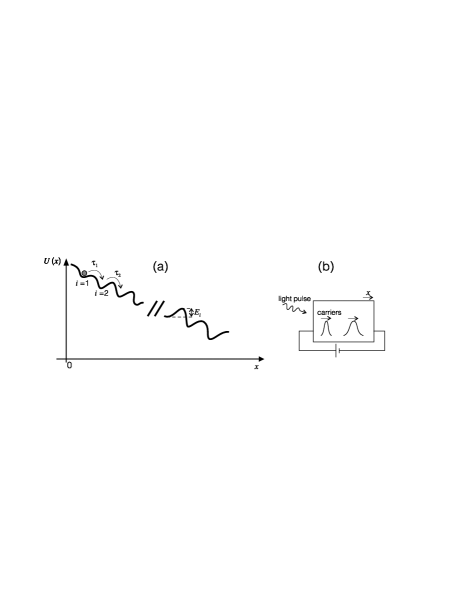
Figure 1: Biased random walks in a disordered system (a) Arrhenius cascade. Each carrier is put in random potential with a global tilt. It undergoes jumps over barriers of random heights $E_{i}$ from a metastable well to the next one on the right thanks to thermal activation. (b) Photoconductivity setup. At time $t=0$, a light pulse creates carriers in the immediate vicinity of the left electrode of an amorphous sample. The carriers of one sign then move through the sample thanks to an applied electric field. (The carriers of the opposite sign are immediately absorbed by the left electrode.)

The mean lifetime of state $i$, i.e., the mean waiting time before the occurrence of a thermal jump, is given by the Arrhenius law:

$$\bar{\tau}_{i}=\tau_{0}e^{E_{i}/kT}$$ (1)

where $\tau_{0}$ is a time scale, $E_{i}$ is the height of the energy barrier separating state $i$ from state $i+1$, $k$ is the Boltzmann constant and $T$ is the temperature. The potential global tilt is assumed to be large enough to neglect backward jumps from $i$ to $i-1$. The random walk we consider is thus completely biased. The time spent between the metastable states is neglected. For a given barrier height $E_{i}$, the lifetime distribution $\psi(\tau|E_{i})$ is exponential with mean $\bar{\tau}_{i}$:

$$\psi(\tau|E_{i})=\frac{1}{\bar{\tau}_{i}}\ e^{-\tau/\bar{\tau}_{i}}.$$ (2)

In the photoconductivity experiments (Fig. 1b), a light pulse creates at time $t=0$ carriers localized near the surface of the sample. The carriers then move through the disordered sample thanks to an applied electric field. Thus, this situation can be modelled by a large number of Arrhenius cascade in parallel, each electron path being associated to one cascade.

One may (wrongly) expect that the transient current flowing through the sample is quasi-constant at the beginning, while the bunch of carriers propagates through the sample, before decreasing rapidly to zero when the carriers leave the sample after reaching the end electrode. But what is observed is quite different. The current decreases as a power law $\sim 1/t^{1-\alpha}$ while the carriers are still in the sample, then as $\sim 1/t^{1+\alpha}$ when some carriers start leaving the sample. For simplicity, we assume here that the sample is semi-infinite so that the carriers never leave the sample.

The explanation of this anomalous behaviour will be shown to be related to the distribution of lifetimes $\tau_{i}$. The randomness of the $\tau_{i}$’s results from the combination of the exponential statistics of jump times for a given barrier height $E_{i}$ (eq. (2)) with the barrier height statistics conveniently described by an exponential distribution $P(E_{i})$,

$$P(E_{i})=\frac{1}{E_{0}}\ e^{-E_{i}/E_{0}}\quad\mathrm{for}\quad E_{i}\geq 0,$$ (3)

where $E_{0}$ is an energy scale related to the sample disorder.

The waiting time distribution $\psi(\tau)$ is then

$$\psi(\tau)=\int_{0}^{\infty}\mathrm{d}E_{i}\ P(E_{i})\psi(\tau|E_{i})=\alpha\gamma(1+\alpha,\tau/\tau_{0})\ \frac{\tau_{0}^{\alpha}}{\tau^{1+\alpha}}$$ (4)

where $\gamma(\alpha^{\prime},x)=\int_{0}^{x}e^{-u}u^{\alpha^{\prime}-1}\mathrm{d}u$ is the incomplete gamma function and

$$\alpha=\frac{kT}{E_{0}}.$$ (5)

At long times, $\psi(\tau)$ tends to a power law, hence the term “fractal time random walk”:

$$\psi(\tau)\simeq\alpha^{2}\Gamma(\alpha)\frac{\tau_{0}^{\alpha}}{\tau^{1+\alpha}},$$ (6)

with $\Gamma(\alpha)=\int_{0}^{\infty}u^{\alpha-1}e^{-u}\ \mathrm{d}u$.

If $\alpha\leq 1$, states $i$ have an infinite mean lifetime $\langle\tau\rangle=\int_{0}^{\infty}\tau\psi(\tau)\ \mathrm{d}\tau$. However, they are unstable since they all ultimately decay to the next state $(i+1)$. Usually, unstable states have a well defined and finite mean lifetime. Here, the somewhat paradoxical presence of unstable states with infinite mean lifetimes is at the origin of the striking properties of the fractal time random walk.

I.2 Subrecoil laser cooling

Laser cooling of atomic gases consists in reducing the momentum spread of atoms thanks to momentum exchanges between atoms and photons. Subrecoil laser cooling consists in reducing the momentum spread to less than a single photon momentum, denoted $\hbar k$. This paradoxical goal is achieved by introducing a momentum dependence in the photon scattering rate (see Fig. 2a) so that it decreases strongly or even vanishes in the vicinity of $p=0$, where $p$ denotes the atomic momentum, taken in one dimension for simplicity.

The mechanism of subrecoil cooling is explained in Fig. 2. Any time a photon is absorbed and spontaneously reemitted by an atom, the atomic momentum undergoes a momentum kick on the order of $\hbar k$, which has a random component because spontaneous emission occurs in a random direction. Thus, the repetition of absorption-spontaneous emission cycles generates for the atom a momentum random walk (see Fig. 2b), with momentum dependent waiting times $\tau$ between two kicks. When an atom reaches by chance the vicinity of $p=0$, it tends to stay there a long time. This enables to accumulate atoms at small momenta, i.e., to cool.

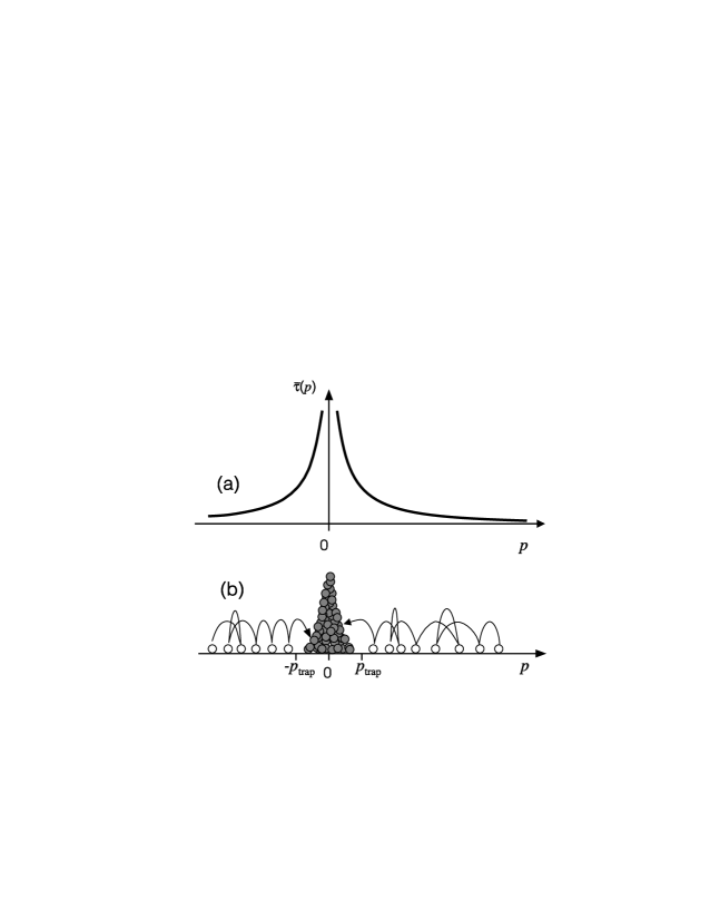
Figure 2: Subrecoil laser cooling (a) The mean sojourn time at momentum $p$ $\bar{\tau}(p)$ becomes very large for small atomic momenta. (b) Photon scattering creates a momentum random walk with an accumulation in the vicinity of $p=0$ due to the momentum dependence of the mean sojourn time $\bar{\tau}(p)$.

For a quantitative treatment, we introduce $\bar{\tau}(p)$, the mean sojourn time at momentum $p$ (also the mean waiting time between two spontaneous photons for an atom at momentum $p$). For a given $p$, the sojourn time at momentum $p$, i.e., the distribution $\psi(\tau|p)$ of sojourn times at momentum $p$ is

$$\psi(\tau|p)=\frac{1}{\bar{\tau}(p)}\ e^{-\tau/\bar{\tau}(p)}.$$ (7)

We need to characterize the distribution of “landing” momenta $\pi(p)$ after a spontaneous emission. Under favourable but often realistic assumptions, atoms spend most of the time around the origin in the interval $[-p_{\mathrm{trap}},+p_{\mathrm{trap}}]$, because they diffuse fast outside this interval and thus come back to it rapidly after leaving it. If $p_{\mathrm{trap}}<\hbar k$, then after a spontaneous emission, the distribution of atomic momenta can be considered as uniform:

$$\pi(p)=\frac{1}{2p_{\mathrm{trap}}}.$$ (8)

The distribution of sojourn times after a spontaneous emission is thus

$$\psi(\tau)=\int_{-p_{\mathrm{trap}}}^{p_{\mathrm{trap}}}\mathrm{d}p\ \pi(p)\psi(\tau|p).$$ (9)

We consider the physically relevant case of power law $\bar{\tau}(p)$,

$$\bar{\tau}(p)=\frac{\tau_{0}p_{0}^{\beta}}{|p|^{\beta}},$$ (10)

where $\beta>0$, and $\tau_{0}$ and $p_{0}$ are time and momentum scales, respectively. Then, one finds, just as in the fractal time random walk, a waiting time distribution with a power law tail:

$$\psi(\tau)=\frac{\alpha p_{0}}{p_{\mathrm{trap}}}\ \gamma\left[1+\alpha,\left(\frac{p_{\mathrm{trap}}}{p_{0}}\right)^{1/\alpha}\frac{\tau}{\tau_{0}}\right]\frac{\tau_{0}^{\alpha}}{\tau^{1+\alpha}}\mathrel{\mathop{\kern 0.0pt\longrightarrow}\limits_{\tau\to\infty}}\alpha^{2}\Gamma(\alpha)\frac{p_{0}}{p_{\mathrm{trap}}}\frac{\tau_{0}^{\alpha}}{\tau^{1+\alpha}},$$ (11)

where

$$\alpha=\frac{1}{\beta}.$$ (12)

If $\beta<1$, the mean waiting time is finite and simple integration gives

$$\langle\tau\rangle=\frac{1}{1-\beta}\left(\frac{p_{0}}{p_{\mathrm{trap}}}\right)^{\beta}\tau_{0}.$$ (13)

If $\beta\geq 1$, on the contrary, the mean waiting time is infinite. This divergence of the mean has dramatic (and positive in terms of cooling) consequences (see §LABEL:s3.2).

I.3 Connection with renewal theory

Renewal processes are stochastic process in which a system undergoes a sequence of events (denoted by $\bullet$ in Fig. 3) separated by independent random “waiting times” $\tau_{1}$, $\tau_{2}$, … The term “renewal process” comes from engineering. Assume that, at time $t=0$, one installs a machine in a factory. When, after being operated for a random lifetime $\tau_{1}$, the machine breaks down, it has to be replaced by a new one, which will work till it breaks down at $\tau_{1}+\tau_{2}$ and has to be replaced … If, instead of a single machine, one has installed a large number of identical machines, then, to decide how many replacement machines must be stored at a given time, one needs to know the replacement rate, which we call hereafter the renewal density.

Figure 3: Renewal processes. The system undergoes a sequence of events (jumps from trap to trap, momentum kicks …) at random times separated by waiting times $\tau_{1}$, $\tau_{2}$, …

To understand the statistical properties of renewal processes, various quantities are introduced. The most detailed information is provided by the distribution of the number of renewals, $f_{t}(r)$, i.e., the probability distribution for the system to undergo $r$ events in time $t$. One also introduces derived quantities, the mean number of renewals at time $t$, $\langle r\rangle_{t}$, and the mean renewal rate at time $t$, denoted $R(t)$ and called the renewal density. Mathematical expressions for these three quantities will be given in §II.1. Here we show the role they play in fractal time random walk and in subrecoil laser cooling.

In the biased (fractal time or non fractal time) random walk, the discretized positions $n$ at time $t$ correspond directly to the number of jumps performed between time $0$ and $t$. Hence the position distribution $\rho(n,t)$ in the fractal time random walk is the renewal number distribution:

$$\rho(n,t)=f_{t}(n).$$ (14)

The mean position of the carriers is $\langle r\rangle_{t}$. The current $i(t)$ measured in photoconductivity experiments before the carriers get out of the sample is proportional to the mean carrier velocity $\mathrm{d}\langle r\rangle_{t}/\mathrm{d}t$, which is the renewal density (see §II.1). Thus, one has

$$i(t)\propto R(t).$$ (15)

In subrecoil cooling, the momentum distribution $\rho(p,t)$ can be written in the following form:

$$\rho(p,t)=\pi(p)\int_{0}^{t}\mathrm{d}t_{l}\ R(t_{l})P_{s}(t-t_{l}|p),$$ (16)

where $t_{l}$ is the time of the last jump occurring between $0$ and $t$, $R(t_{l})\mathrm{d}t_{l}$ is the probability that a jump occurs during the interval $[t_{l},t_{l}+\mathrm{d}t_{l})$, $\pi(p)$ is the uniform probability distribution for a jumping atom to land at momentum $p$ and $P_{s}(t-t_{l}|p)$ is the survival probability for an atom landing at momentum $p$ at time $t_{l}$ to stay there till at least time $t$. Using eq. (7), one has trivially

$$P_{s}(t-t_{l}|p)=\int_{t-t_{l}}^{\infty}\mathrm{d}\tau\ \psi(\tau|p)=e^{-(t-t_{l})/\bar{\tau}(p)}.$$ (17)

The non trivial physical information is contained in the renewal density $R(t)$.

The height $h(t)$ of the momentum distribution peak,

$$h(t)=\rho(p=0,t),$$ (18)

is proportional to $\langle r\rangle_{t}$, the mean number of jumps between $0$ and $t$. Indeed, for any jump, there is a probability $\pi(p)2\mathrm{d}p=\mathrm{d}p/p_{\mathrm{trap}}$ to fall in the vicinity $[-\mathrm{d}p,\mathrm{d}p]$ of the origin and to stay there indefinitely since states in $[-\mathrm{d}p,\mathrm{d}p]$ have arbitrarily long lifetimes in the limit $\mathrm{d}p\to 0$ ($\bar{\tau}(p)\mathrel{\mathop{\kern 0.0pt\longrightarrow}\limits_{p\to 0}}\infty$, see eq. (10)). Thus the height writes

$$h(t)=\frac{\langle r\rangle_{t}}{2p_{\mathrm{trap}}}.$$ (19)

II Renewal theory and Lévy stable laws

II.1 General formulae

The number of renewals $r_{t}$ in a time $t$ is defined as the number of jumps having occurred before time $t$. It satisfies

$$S_{r_{t}}\leq t<S_{r_{t}+1}$$ (20)

where $S_{r_{t}}=\sum_{i=1}^{r_{t}}\tau_{i}$ is the sum of the first $r_{t}$ waiting times. The relationship between the renewal number distribution $f_{t}(r)$ and the waiting time distribution $\psi(\tau)$ can be obtained from the following simple reasoning.

Note first that the distribution, denoted $\psi^{r*}(S_{r})$, of the sum $S_{r}$ of $r$ independent identically distributed waiting times is the $r^{\mathrm{th}}$ convolution product of $\psi(\tau)$ with itself. Moreover, from the definition of the number $r_{t}$ of renewals, one has obviously

$$\mathrm{Pr}(r_{t}<r)=\mathrm{Pr}(S_{r}>t)=\left[1-\Psi^{r*}(t)\right],$$ (21)

where $\Psi^{r*}(S_{r})=\int_{0}^{S_{r}}\psi^{r*}(u)\ \mathrm{d}u$ denotes the distribution function of $S_{r}$ (in spite of its notation, $\Psi^{r*}(S_{r})$ is not the $r^{\mathrm{th}}$ convolution product of the waiting time distribution function $\Psi(\tau)=\int_{0}^{\tau}\psi(u)\ \mathrm{d}u$). The probability distribution $f_{t}(r)$ of the number of renewals at time $t$ is thus finally

$$f_{t}(r_{t}=r)=\mathrm{Pr}(r_{t}<r+1)-\mathrm{Pr}(r_{t}<r)=\Psi^{r*}(t)-\Psi^{(r+1)*}(t).$$ (22)

This expression relates the distribution of a discrete random variable, $r$, to the distribution fonctions of continuous random variables $t$. Important quantities derived from the renewal number distribution $f_{t}(r)$ are the mean number of renewals at time $t$:

$$\langle r\rangle_{t}=\sum_{r=0}^{\infty}rf_{t}(r)$$ (23)

and the renewal density, i.e., the mean number of renewals per unit time